Improving the improved action

Abstract

We investigate the construction of improved actions by the Monte Carlo Renormalization Group method in the context of $SU(2)$ gauge theory utilizing different decimation procedures and effective actions. We demonstrate that the basic self-consistency requirement for correct application of MCRG, i.e. that the decimated configurations are equilibrium configurations of the adopted form of the effective action, can only be achieved by careful fine-tuning of the choice of decimation prescription and/or action.

As it is well-known, the lattice formulation is the only known non-perturbative formulation of gauge theories that gives the path integral in closed form preserving gauge invariance and positivity of the transfer matrix (unitarity). In fact, strictly speaking, the only known way of actually defining ‘continuum’ gauge theory non-perturbatively is by placing the lattice theory on the critical surface of a fixed point of infinite correlation length. Ideally, therefore, one would like to have the action along the Wilsonian ‘renormalized trajectory’ which emanates from the fixed point and proceeds off the critical surface in only the relevant directions. Evolved under successive renormalization group (RG) transformations (‘block-spinnings’), this ‘perfect action’ could therefore be used to compute directly at any scale (coarser lattices) without any contamination from irrelevant directions, and hence any regularization artifacts, and correspondingly greatly reduced computational effort. Concrete practical implementation of this dream, however, turns out to be rather difficult [1].

A more modest approach is based on the fact that the RG trajectory starting at any suitable lattice action will evolve asymptotically to the renormalized trajectory. Thus, after successive block spinnings one should in principle arrive at an ‘improved action’ which allows computation on coarser lattices with suppressed discretization errors. A way to implement this is through the use of the Monte Carlo RG (MCRG) in which one performs block-spinning (decimation) transformations on gauge field configurations obtained by Monte Carlo simulations. The basic postulate here is that the decimated configurations are distributed according to the Boltzmann weight of an effective action that resulted from blocking to the coarser lattice. One, however, does not know a priori what this action is. Given a particular block-spinning prescription, the general procedure that has been followed is to assume a form of the effective action restricted to some subspace of possible interactions [2], and then measure the couplings in this action on the decimated configurations by one of the known methods, the demon [3] or the ‘Schwinger-Dyson’ method [4].

The purpose of this letter is to point out that, given a choice of decimation prescription and a choice of an effective action, straightforward measurement of couplings on the decimated configurations will, in general, lead to erroneous results. This is because the decimated configurations will not be equilibrium configurations of the effective action at these couplings. Surprisingly, this basic requirement underlying MCRG appears not to have been enforced in its application to gauge theories. Careful fine-tuning of the decimation prescription and/or the effective action is required to satisfy this requirement, if it can be satisfied at all within the chosen class of decimation procedures and effective actions.

We demonstrate the presence of the problem and how it can be resolved in $SU(2)$ gauge theory by exploring two different decimation prescriptions: the Swendsen (S) decimation [5], and the ‘Double Smeared Blocking’ (DSB) decimation [6]. Both prescriptions involve a free parameter, $c$, which is the weight of staples relative to straight paths in the construction of the decimated lattice bond variable out of the undecimated lattice ones. We also explore two different effective action models that have been proposed in the literature: the multiple-representation single plaquette action [7], [8], [9]

$$S_{1}=\sum_{plaq}\sum_{j=1/2}^{j_{N}}\beta_{j}[1-\frac{1}{d_{j}}\chi_{j}(U_{p})],$$ (1)

and the action [10]

$$S_{2}=\sum_{plaq}\beta_{11}[1-\frac{1}{2}\chi_{1/2}(U_{p})]+\sum_{rect}\beta_{12}[1-\frac{1}{2}\chi_{1/2}(U_{1\times 2})],$$ (2)

containing the single plaquette ($p=1\times 1$ loop) and the $1\times 2$ planar loop in the fundamental representation. Here $\chi_{j}$ denotes the character of the spin-$j$ representation. We use the demon method to measure couplings.

in	$\beta_{1/2}=\beta_{11}=$2.2578	$\beta_{1}=\beta_{12}=$-0.2201
demon	$\beta_{1/2}=$2.2582(4)	$\beta_{1}=$-0.2203(3)
demon	$\beta_{11}=$2.2576(3)	$\beta_{12}=$-0.2201(1)

Table 1: Measurements of couplings by the demon method before decimation.

To check the ability of the demon to measure couplings correctly, ensembles of 20000 configurations for the action (1), with $j_{N}=1$, and (2) with couplings listed in the first row of Table 1 were generated on a $8^{4}$ lattice. The demon is allowed 1 sweep to set the initial energy, then 10 sweeps for each configuration for measurements. The results, shown in rows 2 and 3 of Table 1, demonstrate that the couplings are indeed accurately reproduced, though at a greater computational cost for (2).

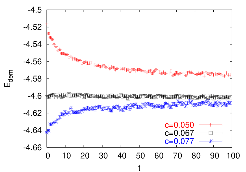
Figure 1: Demon fundamental representation energy flow for DSB decimation and action (1) at various $c$ values.

Starting now with the Wilson action at coupling $\beta=2.5$ on a $32^{4}$ lattice, we perform decimations with scale factor of $2$. Then, adopting one of the effective actions (1) or (2), we proceed to measure the effective action couplings on the decimated configurations by unleashing the demon. We first consider action (1) with $j_{N}=5/2$. Fig. 1 shows the demon fundamental representation energy as a function of sweeps for three values of $c$ for a DSB decimation. The prevalent feature of this plot is that there is significant energy flow during microcanonical evolution for two of the $c$ values shown. There is flow stabilization (equilibration) after about $100$ sweeps. This is in fact the behavior observed for any general $c$ value. Furthermore, this general flow pattern is typical for other representations [9].

The implication of this is clear. Suppose one, working at some chosen $c$ value, measures the couplings for the effective model from the decimated configurations after one or a few demon sweeps (i.e. on the configurations as obtained right after the decimation), and proceeds to generate thermalized configurations of the effective action at these couplings. The decimated configurations will then not be representative of these effective action equilibrium configurations. As seen in Fig. 1 the decimated configurations will evolve under microcanonical evolution towards equilibration at a set of different values for the couplings of the effective action. But by then these evolved configurations no longer are the true original decimated configurations obtained from the underlying finer lattice, and cannot be generally expected to reliably preserve the information encoded in the original configurations.

Ideally, one would like to have for the measurement of couplings on the decimated configurations the same situation as that seen in the test measurement of couplings on the undecimated configurations (cf. Table 1 above), i.e. very fast demon thermalization indicating that the configurations are equilibrium configurations of the action for which the couplings are being measured. The only way out then is to seek a $c$, if any, for which this is realized. In the present case there is one such value, $c\in[0.065,0.067]$, as seen in Fig. 1. Furthermore, this value shows no significant flow, indicating very rapid thermalization, also for the other, in particular, the adjoint representation [9].

A very similar state of affairs is obtained when S decimations are used in conjunction with (1), but the resulting fine-tuning through selection of a $c$-parameter value is not as sharp [11]. Overall, then, DSB is better suited for the action (1), and can be fine-tuned so that decimated configurations are representative of equilibrium configurations of this action.

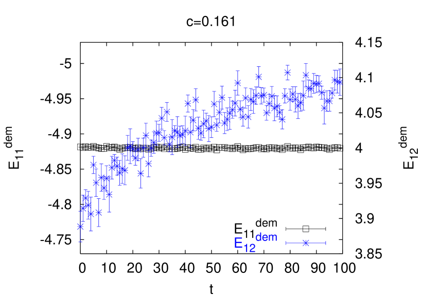
Figure 2: Demon $1\times 1$ and $1\times 2$ loop energy flow for DSB decimation at $c=0.161$.

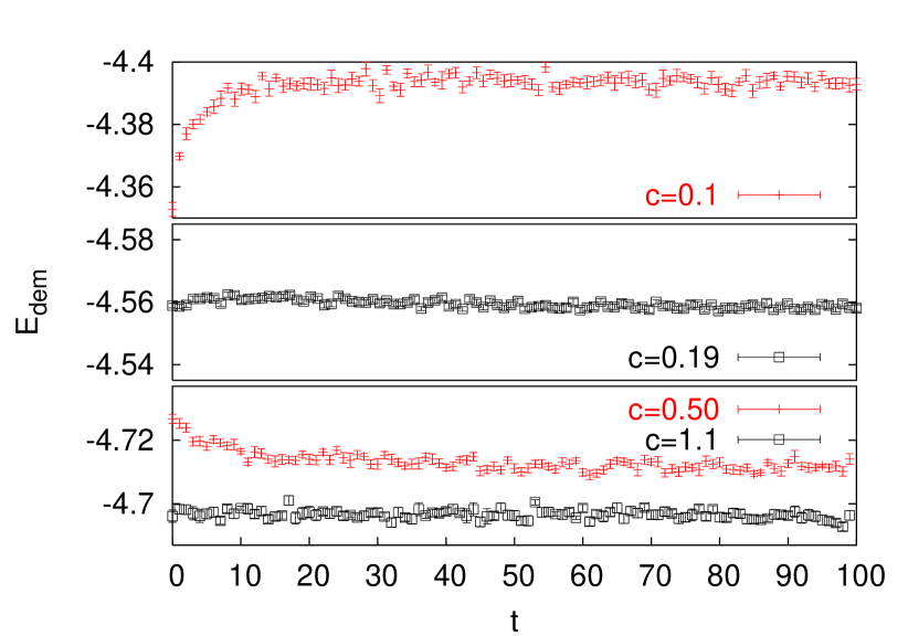
Figure 3: Demon $1\times 1$ loop energy flow for Swendsen decimation at various $c$ values.

We now turn to the action (2). Employing DSB decimation, one again finds the same general picture for general values of the parameter $c$, i.e. significant flow of both the demon plaquette energy $E_{11}$ and $1\times 2$ loop energy $E_{12}$. There are two special $c$ values, $c=0.063(2)$ and $c=0.161(1)$, around which there is nearly no $E_{11}$ energy flow, the second one being much more sharply defined. There is, however, significant flow for the $E_{12}$ demon energy at both values. This is shown for $c=0.161(1)$ in Fig. 2. Similar but stronger flow for $E_{12}$ is observed for $c=0.063(2)$ as well. The only $c$ value for which $E_{12}$ is constant is $c=0.150(2)$, but $E_{11}$ shows strong flow there. It appears that there is no $c$ value for which DSB decimations can be fine-tuned so that the decimated configurations are representative of equilibrium configurations of the effective action (2).

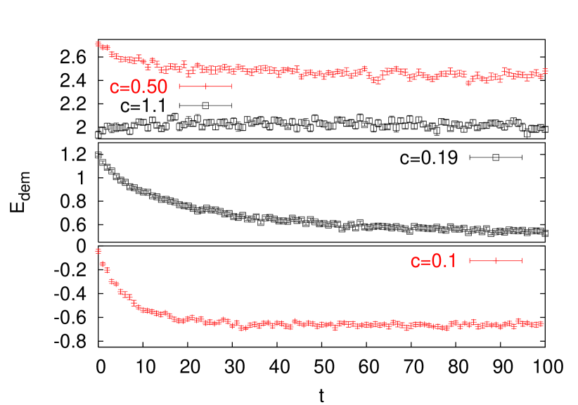
Figure 4: Demon $1\times 2$ loop energy flow for Swendsen decimation at various $c$ values.

Next we consider Swendsen decimations with effective action (2). Figs. 3 and 4 present typical evolution of demon $E_{11}$ and $E_{12}$ energies for various $c$ values. One sees from Fig. 3 that there is approximately no $E_{11}$ flow for $c=0.19(1)$ and $c=1.1(1)$. For the first value, however, there is a significant $E_{12}$ energy evolution as seen in Fig. 4. Thus only the latter value can be used. It appears then that S decimation at $c=1.1$ results in decimated configurations that are nearly equilibrium configurations of (2).

For both DSB and S decimations with effective action (2), the $c$-dependence of demon energies is not monotonic. E.g. for DSB decimation, $E_{11}$ first it goes down, then up with increasing $c$. Similar behavior is seen with S decimations (though this is not apparent in the selection of $c$-values shown in Fig. 3). Furthermore, the direction of the variation for $E_{11}$ is not consistent with that for $E_{12}$, as can be seen from Figs. 3 and 4. This is in contrast to the case of (1) where the demon energies vary monotonically and consistently for various representations and over smaller energy ranges. Furthermore, this picture is stable under addition of higher representation terms. This problem with action (2) may suggest that it is in fact unstable under additions of other terms in the same class of interactions, e.g. other loops of length size (up to) $2$ and/or other representations.

$c$	couplings	$R_{1\times 1}$	$R_{2\times 2}$	$R_{3\times 3}$	$R_{4\times 4}$
0.065	2.5023(7),-0.3098(12)
	0.1057(16), -0.0397(16)	-0.0030(1)	0.1305(9)	0.106(3)	-0.034(14)
	0.0145(14),-0.0029(15)
1.1	3.2925(6),-0.2703(2)	-0.0013(1)	-0.0096(7)	-0.115(2)	-0.252(7)

Table 2: Demon-measured couplings and difference of various size Wilson loops measured on decimated versus effective-action-generated configurations. First row: action (1) with $j_{N}=3$ (six representations); second row: action (2).

To investigate this, and, more generally, the efficacy of (1), (2) as medium to long range effective actions, we consider some observables. In particular, for each of the actions (1), (2), we compare $N\times N$ loops measured in two ways: (a) on the decimated configurations right after the decimations, and denoted $W_{N\times N}^{dec}$; (b) on configurations generated with the effective action at couplings measured after decimation at the optimal $c$-value (DSB for (1), S for (2)), and denoted $W_{N\times N}^{gen}$. The results for the difference

$$R_{N\times N}={\Delta W_{N\times N}\over W_{N\times N}^{dec}}={W_{N\times N}^{gen}-W_{N\times N}^{dec}\over W_{N\times N}^{dec}}$$ (3)

are displayed in Table 2 and plotted in Fig. 5. In contrast to action (1), action (2) shows consistent growth of the difference $R_{N\times N}$ with increasing $N$. It is apparent from these results that action (2) is failing as an accurate intermediate to long scale effective action, and must presumably be augmented by additional terms.

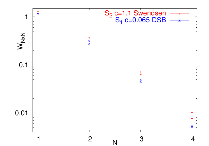
Figure 5: $N\times N$ loop differences defined in eq. (3). From Table 2.

In conclusion, the basic self-consistency requirement for correct application of MCRG is that the decimated configurations are already equilibrium configurations of the adopted form of the effective action at the couplings obtained from the decimated configurations. Careful fine-tuning of the decimation prescription and/or the effective action form is required in order to achieve this. More elaborate decimation prescriptions than the simple DSB and S may be defined, which involve more than one adjustable parameter, and provide more fine-tuning control. Furthermore, more involved actions, e.g. combination of (1) and (2), may be considered. In particular, this program is still to be carried out for the construction of a reliable truly improved $SU(3)$ effective action over a wide range regime.

References

- [1] P. Hasenfratz, Nucl. Phys. Proc. Suppl. 63, 53 (1998) [arXiv:hep-lat/9709110]; W. Bietenholz, [arXiv:hep-lat/9802014].
- [2] An analysis of the effects of such truncation has been given in: T. Takaishi and P. de Forcrand, Phys. Lett. B 428, 157 (1998) [arXiv:hep-lat/9802019].
- [3] M. Creutz, Phys. Rev. Lett. 50, 1411 (1983); M. Creutz, A. Gocksch, M. Ogilvie and M. Okawa, ibid 53, 875 (1984); M. Hasenbusch, K. Pinn and C. Wieczerkowski, Phys. Lett. B 338, 308 (1994) [arXiv:hep-lat/9406019].
- [4] A. Gonzalez-Arroyo and M. Okawa, Phys. Rev. D 35, 672 (1987);
- [5] R. H. Swendsen, Phys. Rev. Lett. 47, 1775 (1981).
- [6] T. A. DeGrand, A. Hasenfratz, P. Hasenfratz, F. Niedermayer and U. Wiese, Nucl. Phys. Proc. Suppl. 42, 67 (1995) [arXiv:hep-lat/9412058]; T. Takaishi, Mod. Phys. Lett. A 10, 503 (1995).
- [7] M. Hasenbusch and S. Necco, JHEP 0408, 005 (2004) [arXiv:hep-lat/0405012].
- [8] E. T. Tomboulis, PoS LAT2005, 311 (2006) [arXiv:hep-lat/0509116].
- [9] E. T. Tomboulis and A. Velytsky, arXiv:hep-lat/0702015.
- [10] P. de Forcrand et al. [QCD-TARO Collaboration], Nucl. Phys. B 577, 263 (2000) [arXiv:hep-lat/9911033].
- [11] See [9] for more extensive discussion and presentation of data for the action (1).