Renormalization Group Therapy

Abstract

We point out a general problem with the procedures commonly used to obtain improved actions from MCRG decimated configurations. Straightforward measurement of the couplings from the decimated configurations, by one of the known methods, can result into actions that do not correctly reproduce the physics on the undecimated lattice. This is because the decimated configurations are generally not representative of the equilibrium configurations of the assumed form of the effective action at the measured couplings. Curing this involves fine-tuning of the chosen MCRG decimation procedure, which is also dependent on the form assumed for the effective action. We illustrate this in decimation studies of the SU(2) LGT using Swendsen and Double Smeared Blocking decimation procedures. A single-plaquette improved action involving five group representations and free of this pathology is given.

1 Introduction

The construction of ‘improved actions’ which reduce discretization errors and allow computation on coarser lattices has been a long-standing area of interest among lattice field theory workers. Ideally, one searches for the ‘perfect action’ ([1] and references within), for which, under successive blocking transformations, the flow is along the Wilsonian ‘renormalized trajectory’, and lattice artifacts disappear. Explicit construction, however, has proved rather cumbersome.

A more modest but more readily implementable approach is based on the Monte Carlo Renormalization Group (MCRG) which considers block spinning transformations on configurations obtained by MC simulations. The basic assumption here is that the block-spinned configurations are distributed according to the Boltzmann weight of some effective action that resulted from the blocking to the coarser lattice. One, however, does not know at the outset what this block effective action is. Now, under RG evolution any starting action generally develops a variety of additional couplings. An adequate model of the resulting effective action must, therefore, include a choice of several such couplings. By practical necessity, any Ansatz for such a model is restricted to some subclass of possible interactions. In the past effective models have been studied with actions consisting of one or more loops beyond the single plaquette in the fundamental representation [2], or a mixed fundamental-adjoint single plaquette action [3], [4]. After a block spinning is performed starting from a simple (e.g. Wilson) action, one needs to measure the set of couplings retained in one’s model of the effective action. This may be achieved by the use of demon [5] or Schwinger-Dyson methods [6].

There is a variety of issues that come up in the actual implementation of such a program. Any numerical decimation procedure entails some mutilation and possible loss of information encoded in the original undecimated configurations. The first thing to be checked then is that the adopted decimation prescription correctly reproduces physics at least at intermediate and long distance scales.

Assuming this is the case, some effective action must next be assumed. It should be noted that the issue of the choice of an effective action model is not divorced from the choice of the decimation procedure. Indeed, in any exact RG transformation, the particular specification, in terms of the original variables, of the blocking procedure and block variables will affect the form of the action which results after integration over the original variables. Thus different decimation procedures, or even different regimes of the parameters entering the specification of one particular decimation procedure, may be fitted better by different effective action models.

Having adopted some class of effective actions, errors due to the truncation of the phase space inherent in any such choice may, of course, be significant, and prevent the model from adequately approaching the renormalized trajectory. This is something that one can in principle check by measurement of appropriate observables probing the scale regime(s) of interest, and may result in the need for addition of further effective couplings.

There is, however, a more subtle pitfall lurking in a straightforward application of such methods. A straightforward ‘measurement’ of the effective action couplings from the decimated configurations, by any one of the available methods, can actually lead to quite erroneous results. This is because the decimated configurations will generally not be representative of the equilibrium configurations of the effective action at the measured couplings. As a result simulations on the coarser lattice with the effective action at these values of the couplings will not, in general, correctly reproduce the physics encoded in the decimated configurations obtained from the original theory. As far as we know, this does not appear to have been realized in previous MCRG gauge theory studies. In this paper we find that this problem is actually generally present and has to be dealt with. We use the demon method which provides a clear demonstration of the problem as it allows comparison between the original decimated and microcanonically-evolved decimated configurations in relation to equilibrium configurations of the assumed effective action.

Specifically, we explore these issues in numerical decimations in $SU(2)$ LGT. A preliminary report on some of our findings was previously given in [7]. The present paper is organized as follows. In section 2 we introduce different decimation schemes, as well as the numerical methods we use to implement them. We check that the decimation procedures correctly reproduce long distance physics. We then adopt a single plaquette effective action which includes several (typically five to eight) successive group representations. There are special motivations for such actions originating in exact analytical results. In section 3 we present the results of our numerical study. We examine the relation between the configurations obtained by decimation from the original action and the thermalized configurations of the effective action. We explore how this affects the determination of the effective couplings and the tuning of the free parameters (such as the relative weight of staples) entering in the specification of the decimation scheme. We then examine how physics is reproduced by measuring observables such as Wilson loops of various sizes. The behavior under repeated decimation is also examined. In section 4 we extract from our results our improved action. Our conclusions and outlook are summarized in section 5.

2 Decimation procedures

In our study we choose to start with the standard Wilson action with coupling $\beta$ on the original undecimated lattice. Throughout this paper we use blocking $a\to ba$ with scale factor $b=2$ in all lattice directions. We employ two well-known numerical blocking procedures. In terms of the usual lattice gauge field bond variables $U_{\mu}(n)$, these are:

• Swendsen decimation [9]

  $$Q_{\mu}(n)=U_{\mu}(n)U_{\mu}(n+\hat{\mu})+c\sum_{\nu\neq\mu}U_{\nu}(n)U_{\mu}(n+\hat{\nu})U_{\mu}(n+\hat{\nu}+\hat{\mu})U_{-\nu}(n+\hat{\nu}+2\hat{\mu})$$ (1)

• Double Smeared Blocking (DSB)[10]

  $$U_{\mu}(n) = (1-6c)U_{\mu}(n)+c\sum_{\nu\neq\mu}U_{\nu}(n)U_{\mu}(n+\hat{\nu})U^{\dagger}_{\nu}(n+\hat{\mu})\quad\times 2\,{\rm times}$$

  $$Q_{\mu}(n) = U_{\mu}(n)U_{\mu}(n+\hat{\mu}).$$ (2)

Here $c$ is a parameter which controls the relative weight of staples. For Swendsen decimation the values $c=0.5$ and $1$ [2, 9], whereas for double smeared blocking the classical limit value $c=0.077$ [11] have previously been used. Fixing the parameter $c$ on a rational rather than ad-hoc basis will be one of our concerns below.

As a typical check on how such decimations preserve the information in the original undecimated configurations, at least at long distances, we look at the quark potential. The original lattice potential was computed with high accuracy (20 independent runs each consisting of 300 measurements) using the Lüscher-Weisz procedure [12], while the decimated potentials were computed in the straightforward ’naive’ way, which affects their accuracy, but suffices for a check (from 80 to 160 independent runs each of 3000 measurements). The result of the comparison for Swendsen decimation is given in Table 1, with average goodness of fit $Q\sim 0.6$.

$c$	$\mu$	$\sigma$
orig	0.308(4)	0.0313(2)
0.1	0.67(13)	0.020(4)
0.12	0.71(12)	0.019(4)
0.2	0.33(7)	0.031(2)
0.26	0.39(4)	0.029(1)
0.3	0.39(2)	0.0292(7)
0.5	0.36(2)	0.0301(9)
1.0	0.33(2)	0.0314(6)

Table 1: String tension $\sigma$ and Coulomb term coefficient $\mu$ computed on the original and decimated lattices. Swendsen decimation, $\beta=2.5$.

One can note that for a wide range of $c$ starting from value $\sim 0.2$ all the decimations produce correct values of string tension $\sigma$. The Coulomb term coefficient $\mu$, however, which is representative of short distance physics, does show distortion due to the decimation procedure. Such short distance distortions are typical of numerical decimation procedures. One is interested in extracting an effective action that is good at intermediate and long scales.

After blocking, we need to assume some model of the effective action. We take a single plaquette action

$$S=\sum_{j=1/2}^{N_{r}}\beta_{j}[1-\frac{1}{d_{j}}\chi_{j}(U_{p})],$$ (3)

truncated at some high representation $N_{r}$ as our general form of the effective action. (As usual, in (3) $U_{p}$ denotes the product of the bond variables along the boundary of the plaquette $p$.)

The choice (3) is motivated by some exact analytical results [8]. There are decimation transformations of the ‘potential moving’ type characterized by one or more free parameters which, after each blocking step, preserve a single plaquette action of the type (3) albeit with the full (infinite) set of representations. By appropriate choice of the decimation transformation parameter(s), the partition function obtained after a blocking step can be made to be either an upper or a lower bound on the original partition function. It is then possible to introduce a single parameter which, at each decimation step, interpolates between the upper and lower bound, and hence has a value that keeps the partition function constant, i.e. exact under each successive decimation step. The same result can be obtained for ‘twisted’ partition function (partition functions in the presence of external fluxes) and some other related long-distance quantities. This means that the action (3) can in principle reproduce the exact partition function and other judiciously chosen quantities under successive blockings.

To compare the effective action model to the decimated original theory, we need an efficient way to simulate a gauge theory with action (3). We use a procedure due to Hasenbusch and Necco [4]. The fundamental representation part of the action with specially tuned coupling is used to generate trial matrices for the metropolis updating. This procedure typically achieves $80\%$ acceptance rate for the metropolis algorithm at the used couplings. Alternatively one could use a newly developed biased metropolis algorithm [13]. Simple heatbath updating is used only in the case of the action restricted to only the fundamental representation.

To measure couplings we use the microcanonical evolution method [5]. For the microcanonical updating and demon measurements we implement an improved algorithm given in [14]. The demons energies are restricted to $[-E_{max},$ $E_{max}]$, thus preventing demons from ‘running away’ with all the energy. We use $E_{max}=5$ value. The couplings $\beta_{j}$ of the effective action can be obtained as solutions of the equation

$$\langle E^{d}_{j}\rangle=1/\beta_{j}-E_{max}/tanh[\beta_{j}E_{max}],$$ (4)

where $E^{d}_{j}$ denotes the corresponding demon energy. In table (2) we demonstrate the ability of the canonical demon method in measuring the couplings on $8^{4}$ lattice. An ensemble of $3000$ configurations with couplings listed in the first row of the table is used. Demon is allowed 1 sweep for reaching equilibrium, than 10 sweeps for measurements. The measured couplings are listed on the second row of the table and are in good agreement with the initial values.

	$\beta_{1/2}$	$\beta_{1}$	$\beta_{3/2}$	$\beta_{2}$	$\beta_{5/2}$
in	2.2578	-0.2201	0.0898	-0.0333	0.0125
demon	2.2580(4)	-0.2206(4)	0.0903(5)	-0.0336(5)	0.0127(4)

Table 2: Measurements of couplings by canonical demon method.

3 Decimation study

We fix the effective action to have 8 consecutive representations, starting from the fundamental. For consecutive Monte Carlo updating of the effective action we truncated the number of couplings to the first five. A $32^{4}$ lattice at $\beta=2.5$ is decimated once, using Swendsen type decimation with various staple weights $c$. In Fig. 1 we show the fundamental representation demon energy flow, starting from $c=0.1$ Swendsen decimated configurations. For the demon energy flow measurements we typically use from 20 to 100 replicas (identical runs with different initial random number generator seeds).

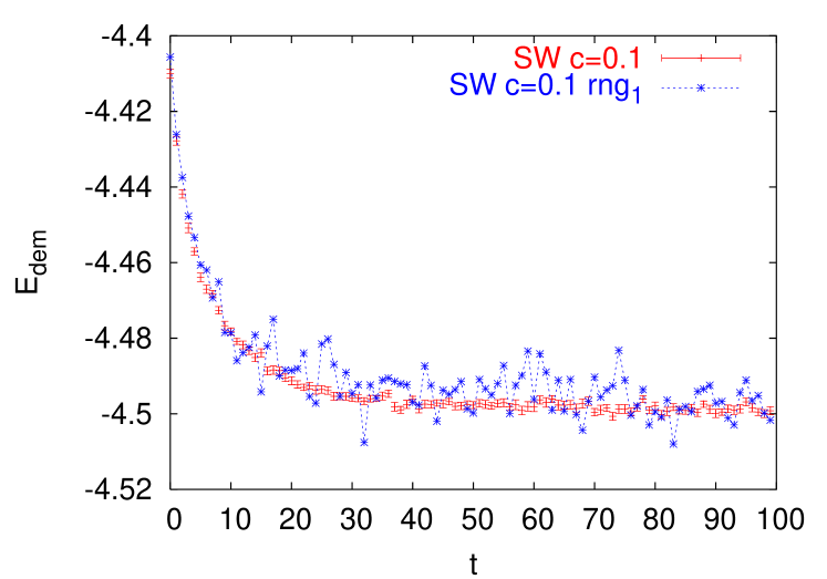
Figure 1: Demon fundamental representation energy flow for $c=0.1$ Swendsen decimated configurations. The average and a single demon run.

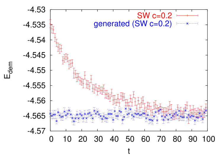
Figure 2: Demon fundamental representation energy flow for $c=0.2$ Swendsen decimated configurations and for configurations generated with an effective action.

The obvious main feature in this plot is that there is a significant demon energy change during microcanonical evolution. The change for different replicas is always in the same direction. There is a noticeable trend for flow stabilization at $\sim 100$ sweeps.

Next, taking $c=0.2$, we let the demon reach equilibrium ($>100$ sweeps) and then measure the couplings of the effective action (3). We then simulate the effective action at these couplings and generate thermalized configurations for it. We then compare the demon evolution on these thermalized configurations with the demon evolution on the $c=0.2$ Swendsen decimated configurations (Fig 2). There is now a striking difference. We see that in the case of the thermalized configurations of the effective action there is no change in the demon energy, which indicates a very fast demon equilibration. Whereas in the case of the decimated configurations there is a pronounced energy change (as we also saw with the $c=0.1$ Swendsen decimated configurations). This pronounced energy change is clearly due to configuration equilibration during microcanonical evolution. This evolutions eventually brings the original decimated configurations towards equilibrium configurations of the effective model.

The implication of this is obvious. Suppose one measures the couplings for the effective model from the decimated configurations after one or a few demon sweeps (i.e. on the configurations as obtained right after the decimation). These couplings are given in the first entry of the first column of Table 3 below. Suppose one generates thermalized configurations of the effective action at these couplings. Then the decimated configurations are not representative of these effective action equilibrium configurations. As we saw the decimated configurations will evolve under microcanonical evolution towards equilibration at a set of different values for the couplings of the effective action. But by then they no longer are the true original decimated configurations obtained from the underlying finer lattice.

This clearly would appear to present a potentially serious problem. It means that MC simulations using the effective action with coupling measured on the decimated configurations will not in general reproduce results from measurements obtained from the decimated configurations. Sufficient microcanonical evolution has to occur on the decimated configurations in order to ‘project’ them into the equilibrium configurations of the effective model at some (other) set of couplings. It is an interesting question to what extent these evolved decimated configurations still retain any useful information concerning the starting action on the finer lattice. We come back to this point in subsection 3.1 below.

The obvious next question is whether one can address this problem by fine-tuning the decimation procedure. Ideally, one would like to have for the measurement of couplings on the decimated configurations the same situation as that seen in the measurement of couplings on the undecimated configurations (cf. Table 2 above), i.e. very fast demon thermalization indicating that the configurations are equilibrium configurations of the action for which the couplings are being measured.

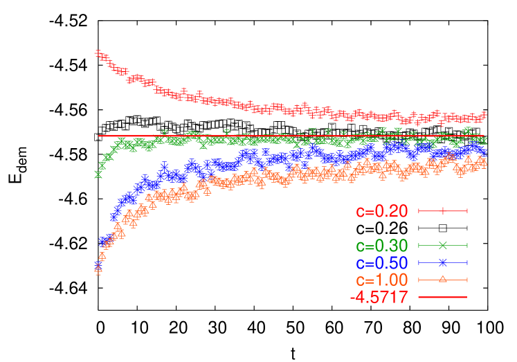
Figure 3: Demon fundamental representation energy flow for Swendsen decimation at various $c$ values.

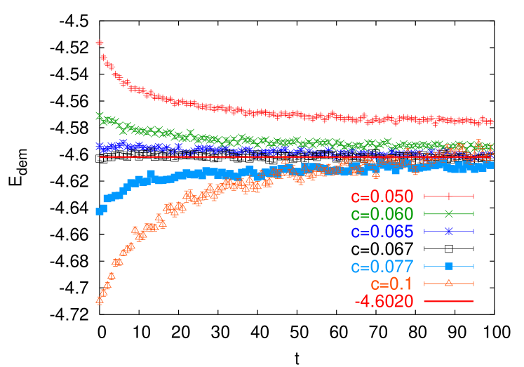
Figure 4: Demon fundamental representation energy flow for DSB decimation at various $c$ values.

The only freedom in the specification of the decimations (1), (2) is the staple weight parameter $c$. We then vary $c$ and observe the demon energy flow. In Fig. 3 we exhibit the fundamental demon energy evolution for $c=0.2,\ldots,1.0$ Swendsen decimations. We observe that there is a special $c\approx 0.26$ value, when right from the start there is little demon energy change. These particular decimation configurations are then very close to the equilibrium configuration of the action (3). In Fig 4 we show the fundamental demon energy flow for DSB decimations with $c=0.050,\ldots,0.1$. Again, there is a special value in the vicinity $c\sim 0.067$ for which there is no significant flow from the outset.

In Figs. 5, 6 we look at the adjoint demon energy flows for Swendsen and DSB decimations, respectively. For Swendsen decimations we notice that now there is a small change for $c=0.26$, while no appreciable flow for $c=0.3$. For DSB decimations there appears to be no discernible shift in the vicinity of the optimal $c$ value.

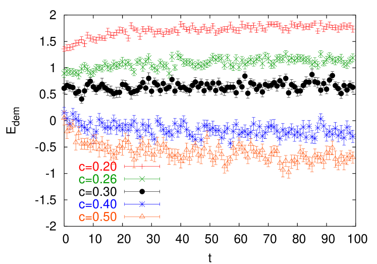
Figure 5: Demon adjoint representation energy flow for Swendsen decimation at various $c$ values.

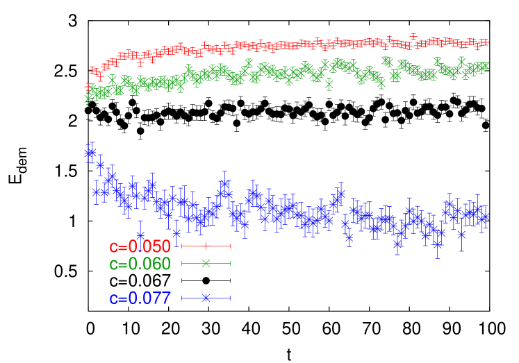
Figure 6: Demon adjoint representation energy flow for DSB decimation at various $c$ values.

This is the first indication that DSB decimation is better suited for the effective action (3).

3.1 Observables

We next compare some medium scale physical observables measured on the decimated configurations (right after decimation) and on configurations obtained from the effective action as described below.

First, for $c=0.2$ Swendsen decimation, we take the effective action with couplings obtained by demon measurements immediately after the decimation. We then compute $N\times N$ Wilson loops measured in two ways: (a) on the decimated configuration immediately after the decimation, denoted $W_{N\times N}^{dec}$; and (b) on configurations generated with this effective action, denoted $W_{N\times N}^{gen}$. The difference

$${\Delta W_{N\times N}\over W_{N\times N}^{dec}}=\frac{W_{N\times N}^{gen}-W_{N\times N}^{dec}}{W_{N\times N}^{dec}}$$ (5)

is displayed in the first row of Table 3. The second row displays this difference when the effective action is now taken with couplings obtained by demon measurements after 100 sweeps, i.e. at the end of the microcanonical evolution shown in Fig. 2.

$sws/m$	$\beta_{1/2},\beta_{1},\beta_{3/2},\ldots$	$\Delta W_{1\times 1}/W^{dec}_{1\times 1}$	$\Delta W_{2\times 2}/W^{dec}_{2\times 2}$	$\Delta W_{3\times 3}/W^{dec}_{3\times 3}$
0/1	2.1391(5),-0.1628(9),
	0.0637(11),-0.0250(1),	-0.0642(1)	-0.2832(5)	-0.7196(9)
	0.0098(15)
100/20	2.2963(4),-0.2351(5),
	0.0955(7),-0.0357(9),	-0.0045(1)	-0.0296(10)	-0.3912(20)
	0.0131(11),-0.0050(12)

Table 3: Demon-measured couplings after $c=0.2$ Swendsen decimation, and difference of various size Wilson loops measured on decimated versus effective-action-generated configurations. Measurements performed right after the decimation (measurement: 1 sweep) and after 100 sweeps (measurements: 20 sweeps).

The table nicely illustrates the discussion above. One sees that measurements performed with the effective action having couplings obtained from the decimated configurations deviate from the values measured on the decimated configurations themselves (first row). Furthermore, the discrepancy grows substantially with increasing length scale, becoming large for the intermediate scale $3\times 3$ loop. This is in fact the worst possible outcome - it is at intermediate and long scales that the decimated configurations preserve the information on the undecimated lattice. But it is not unexpected since the decimated configurations are not equilibrium configurations of the effective action. There is noticeable improvement, though still not near agreement, when couplings are obtained from microcanonically evolved decimated configurations, which are then equilibrium configurations of the resulting effective action (second row). This seems to imply that the microcanonically evolved decimated configurations, at least for these observables, retain some of information encoded in the original decimated configurations.

We next compute the difference (5) for a range of $c$ values. In these computations we use 30 independent runs of 30 measurements each for the $\beta$ measurements, and $20-30$ independent runs each of 400 measurements for the effective action simulations. The effective action couplings are obtained after $100$ demon sweeps when thermalization is reached (cf. Figs. 1 and 2). The results for Swendsen decimations and for DSB are presented in Table 4 and Table 5, respectively.

$c$	$\beta_{1/2},\beta_{1},\beta_{3/2},\ldots$	$\Delta W_{2\times 2}/W^{dec}_{2\times 2}$	$\Delta W_{3\times 3}/W^{dec}_{3\times 3}$
0.0	1.1340(2),-0.1974(2),
	0.0531(3),-0.0162(4),	-0.8141(4)	-0.9876(39)
	0.0054(3),-0.0020(4)
0.1	1.9912(3),-0.3085(4),
	0.0990(4),-0.0362(6),	-0.4160(6)	-0.8899(11)
	0.0139(7),-0.0045(8)
0.2	2.2963(4),-0.2351(5),
	0.0955(7),-0.0357(9),	-0.0296(10)	-0.3912(20)
	0.0131(11),-0.0050(12)
0.26	2.3351(7),-0.1449(10),
	0.0766(12),-0.0279(13),	0.1502(11)	0.0926(29)
	0.0084(17)
0.3	2.3447(8),-0.0869(12),
	0.0628(14),-0.0236(15),	0.2545(12)	0.4559(41)
	0.0075(20)
0.4	2.3555(9), 0.0229(14),
	0.0301(18),-0.0101(22),	0.4191(14)	1.1763(64)
	0.0016(22)
0.5	2.3618(9),0.0866(13),
	0.0070(17),-0.0027(20),	0.4780(14)	1.5029(69)
	-0.0013(22)
1.0	2.4033(9),0.1150(14),
	-0.0274(18), 0.0071(22),	0.4456(14)	1.4845(75)
	-0.0041(29)

Table 4: Swendsen decimations. Demon-measured couplings at different $c$ values, and difference of various size Wilson loops measured on decimated versus effective-action-generated configurations. Thermalization: 100 sweeps, measurements: 20 sweeps..

$c$	$\beta_{1/2},\beta_{1},\beta_{3/2},\ldots$	$\Delta W_{2\times 2}/W^{dec}_{2\times 2}$	$\Delta W_{3\times 3}/W^{dec}_{3\times 3}$	$\Delta W_{4\times 4}/W^{dec}_{4\times 4}$
0.050	2.3536(5),-0.4208(9)
	0.1430(11),-0.0558(13)	-0.1817(6)	-0.637(1)
	0.0238(13),-0.0094(15)
0.060	2.4660(7),-0.3635(11)
	0.1242(17),-0.0475(21)	0.0105(7)	-0.239(2)
	0.0195(25),-0.0070(24)
0.063	2.4891(7),-0.3331(11)
	0.1140(14),-0.0436(19)	0.0800(9)	-0.049(3)
	0.0180(25),-0.0070(25)
0.065	2.5023(7),-0.3098(12)
	0.1057(16), -0.0397(16)	0.1305(9)	0.106(3)	-0.034(14)
	0.0145(14),-0.0029(15)
0.067	2.5125(7),-0.2832(16)
	0.0964(25),-0.0367(29)	0.1774(9)	0.266(3)	0.290(19)
	0.0139(29)
0.077	2.5463(11),-0.1167(17),	0.4149(14)	1.270(7)
	0.0320(23),-0.0055(28)
0.1	2.4762(20),0.4191(37)
	-0.1231(40),0.0504(39)	0.6558(9)	2.627(6)
	-0.0191(53),0.0063(54)

Table 5: Same as Table 4 for DSB decimations.

Clearly, the $c$ values that give the best results, giving a difference (5) that goes to zero at intermediate size Wilson loops, are precisely those in the vicinity of the values that produce decimated configurations which are closest to equilibrium configurations of the effective action. These are around $c\sim 2.6$ for Swendsen decimations. For DSB decimations the optimal value is between $c>0.065$ and $c<0.067$. This then provides a method of fixing $c$ in (1) and (2). It is interesting to note in particular that the classical $c$ value of DSB produces results which are incapable of reproducing the physics at these scales correctly.

3.2 Other $\beta$’s

$\beta$	1/2	1	1/2	1
2.5	0.26	0.3	0.067	0.068
2.8	0.21	0.22	0.059	0.060
3.0	0.19	0.20	0.056	0.057

Table 6: The $c$ parameter for no demon energy flow in fundamental (1/2) and adjoint (1) representations for Swendsen (left part) and DSB (right part) decimations at different $\beta$’s.

So far we have been working at $\beta=2.5$ (Wilson action) on the undecimated lattice. In Table 6 we list the optimal $c$ values that result in no demon energy flow also for some other $\beta$ values. As expected, the optimal value depends on $\beta$.

Determination of one optimal $c$ appears somewhat less sharp for Swendsen decimations than for DSB decimations. The latter appear better behaved and exhibit more consistency between higher representation demon energy flow and the fundamental energy. Overall, DSB is the better suited decimation procedure for the effective action (3).

3.3 Double decimation

In Figs. 7 and 8 we show the fundamental representation demon energy flow after two successive Swendsen and DSB decimations, respectively, at various $c$ values at $\beta=2.5$. As seen in these plots, the general trend of demon energy flows is the same as after one decimation step. The optimal values for the staple weight $c$, however, differ from those for a single decimation step. For double decimation at $\beta=2.5$ we have optimal $c=0.39$ for Swendsen decimations; and $c=0.078$ for DSB decimations. At $\beta=2.8$, the optimal value for DSB decimations is $c=0.066$.

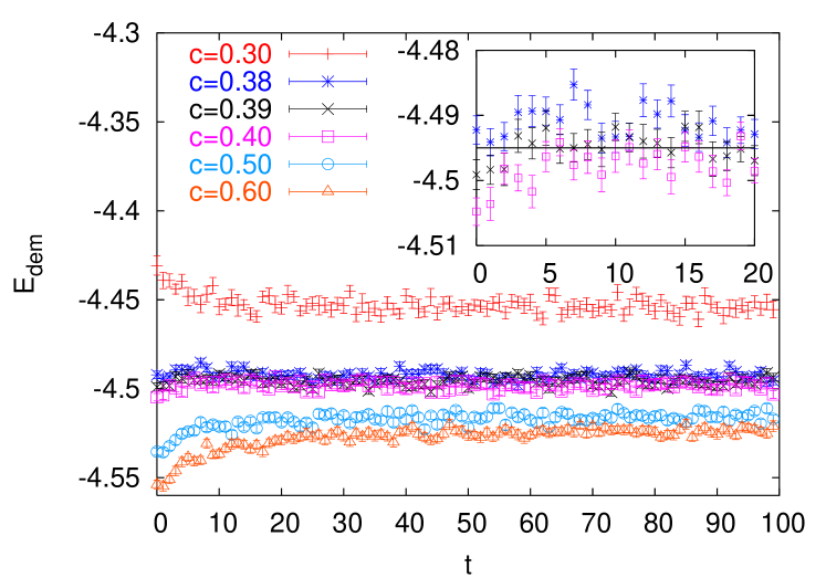
Figure 7: Fundamental representation demon energy flow for double Swendsen decimation at various $c$ values.

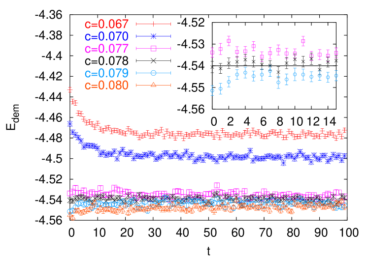
Figure 8: Fundamental representation demon energy flow for double DSB decimation at various $c$ values.

4 Improved action

In this section we extract our improved action from our data. We have chosen DSB over Swendsen type decimation, since, as remarked above, it produces better overall results for the action (3).

We look at 8 coupling in the improved action, and report on first 5 of them. Typically we perform 30 independent runs each of $100-400$ measurements. We present the result in Table 7. At each successive decimation step, enumerated by $n$, we choose the value for the staple weight which results in the minimal fundamental demon energy flow (cf. 4th column of Tab. 6 for the $n=1$ step).

$n$	$c$	$\beta_{1/2}$	$\beta_{1}$	$\beta_{3/2}$	$\beta_{2}$	$\beta_{5/2}$
$\beta=2.5$
1	0.067	2.5125(7)	-0.2832(16)	0.0964(25)	-0.0367(29)	0.0139(29)
2	0.078	2.0110(8)	-0.1351(7)	0.0385(10)	-0.0104(13)	0.0026(13)
3	0.078*	0.8869(4)	-0.0390(4)	0.0067(4)	-0.0007(5)	0.0008(10)
4	0.078*	0.1513(2)	0.0002(4)	-0.0003(5)	-0.0004(7)	0.0009(7)
$\beta=2.8$
1	0.059	2.9841(23)	-0.4649(38)	0.1895(52)	-0.0898(62)	0.0432(65)
2	0.066	2.6658(31)	-0.3943(49)	0.1446(61)	-0.0585(81)	0.0280(96)
3	0.075	2.1773(16)	-0.1959(16)	0.0555(14)	-0.0164(16)	0.0057(23)
$\beta=3.0$
1	0.056	3.2831(37)	-0.5611(53)	0.2397(74)	-0.1193(93)	0.05842(96)
2	0.063	2.9920(54)	-0.4824(97)	0.181(14)	-0.067(18)	0.020(20)

Table 7: Flow of couplings of the DSB decimated (improved) action. $\beta$ is the coupling of the original Wilson action on the original (undecimated) lattice. n enumerates successive decimations. First decimation is from 32 to 16 lattice, then all consecutive decimations are on 16. * means there is in fact virtually no discernible demon flow in reasonable range of $c$ around the indicated value.

In Fig. 9 we plot the RG flow of the first two, i.e. fundamental and adjoint, couplings from Table 7.

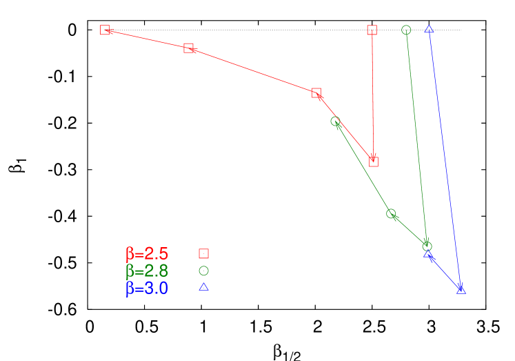
Figure 9: RG flow (from Table 7) under successive DSB decimations projected onto the $\beta_{1/2}$ - $\beta_{1}$ plane.

$c$	$\beta_{1/2},\beta_{1},\beta_{3/2},\ldots$	$\Delta W_{1\times 1}/W^{dec}_{1\times 1}$	$\Delta W_{2\times 2}/W^{dec}_{2\times 2}$	$\Delta W_{3\times 3}/W^{dec}_{3\times 3}$
0.067	2.5125(7),-0.2832(16)
	0.0964(25),-0.0367(29)	-0.0018(1)	0.1774(9)	0.266(3)
	0.0139(29)
0.067	2.4574(5),-0.1824(4)	-0.0012(1)	0.180(1)	0.273(4)

Table 8: Comparison of measurement of 5(8) couplings with only first 2 couplings effective action. DSB decimation at $\beta=2.5$. The first row is taken from Table 5 above.

$\beta$	$\beta_{1/2}$	$\beta_{1}$
2.5	2.4574(5)	-0.1824(4)
2.8	2.8366(6)	-0.2428(4)
3.0	3.0802(9)	-0.2693(6)

Table 9: Couplings of the decimated (improved) action retaining only first 2 representations for DSB decimation at different $\beta$’s.

As a matter of practical expediency, one may want to consider the effective action truncated to just these two couplings at the outset. In Table 8 we compare the results of measurements keeping just the two couplings to those keeping all five (eight). Comparison of the two rows of this table indicates the size of systematic error induced by this truncation of the effective action. The values of the two couplings for different starting $\beta$’s is given in Table 9 to be compared with those in Table 7 ($n=1$).

5 Summary and outlook

We studied MCRG decimations in $SU(2)$ LGT employing either DSB or Swendsen decimations followed by a search for an effective action in the space of multi-representation single-plaquette actions with up to eight couplings using the demon method. Examination of the demon microcanonical evolution on the decimated configurations reveals the following general feature. Given the couplings of the effective action obtained from the decimated configurations, consider the equilibrium configurations of the effective action at these couplings. Then the decimated configurations are not, in general, representative of these equilibrium configurations. This means that simulations with the effective action at these couplings will not reproduce measurements of observables obtained from the decimated configurations as demonstrated in section 3 above.

If sufficient microcanonical evolution of the decimated configurations is allowed, they will eventually result into configurations that are indeed equilibrium configurations of the effective action, that is the effective action at couplings obtained from these evolved decimated configurations. But the evolved decimated configurations are no longer the original decimated configurations, and cannot be relied upon to still adequately encode information from the original undecimated lattice.

Solving this problem means having decimated configurations that are already equilibrium configurations of the adopted form of the effective action at the couplings obtained from the decimated configurations. This in general requires fine-tuning of the decimation and/or the effective action.

In the case of the type of decimations and effective action adopted in this study, we saw that this fine-tuning could be achieved by fixing the value of the staple weight parameter $c$ in the specification of the decimation procedure, and retaining sufficient number of couplings. Also, this tuning works somewhat better for DSB decimations than Swendsen decimations. The result is the improved action presented in Table 7 and Fig. 9. Further improvements and refinements are presumably possible if more elaborate decimations involving more parameters are employed.

Clearly, the general state of affairs described here holds independently of the choice of decimation procedure and/or effective action. In this study we used the multi-representation single-plaquette action. Preliminary data with alternative actions, such as a multiloop fundamental representation action, reveal the same picture as expected.

The use of the demon method for measuring couplings is also immaterial. The alternative Schwinger-Dyson (SD) method could be used. With this latter method, however, one does not have the option of microcanonically evolving the decimated configurations towards equilibration vis-a-vis the effective action, which is very informative and a nice advantage of the demon method. With SD a necessary test is to compare between: (a) the expectations, computed from the decimated configurations, of the operators occurring in the SD equation, which are then used in that equation to obtain the couplings; and (b) the same expectations computed with effective action equilibrium configurations generated at these couplings. We hope to report results employing these alternative choices elsewhere.

Extension of our study to $SU(3)$ to obtain the analog of the $SU(2)$ effective action arrived at here would also be worthwhile.

References

- [1] P. Hasenfratz, Nucl. Phys. Proc. Suppl. 63, 53 (1998) [arXiv:hep-lat/9709110].
- [2] P. de Forcrand et al. [QCD-TARO Collaboration], Nucl. Phys. B 577, 263 (2000) [arXiv:hep-lat/9911033].
- [3] M. Creutz, A. Gocksch, M. Ogilvie and M. Okawa, Phys. Rev. Lett. 53, 875 (1984).
- [4] M. Hasenbusch and S. Necco, JHEP 0408, 005 (2004) [arXiv:hep-lat/0405012].
- [5] M. Creutz, Phys. Rev. Lett. 50, 1411 (1983).
- [6] A. Gonzalez-Arroyo and M. Okawa, Phys. Rev. D 35, 672 (1987); Phys. Rev. B 35, 2108 (1987).
- [7] E. T. Tomboulis and A. Velytsky, PoS LAT2006, 077 (2006) [arXiv:hep-lat/0609047].
- [8] E. T. Tomboulis, PoS LAT2005, 311 (2006) [arXiv:hep-lat/0509116].
- [9] R. H. Swendsen, Phys. Rev. Lett. 47, 1775 (1981).
- [10] T. A. DeGrand, A. Hasenfratz, P. Hasenfratz, F. Niedermayer and U. Wiese, Nucl. Phys. Proc. Suppl. 42, 67 (1995) [arXiv:hep-lat/9412058].
- [11] T. Takaishi, Mod. Phys. Lett. A 10, 503 (1995).
- [12] M. Luscher and P. Weisz, JHEP 0109, 010 (2001) [arXiv:hep-lat/0108014]; JHEP 0207, 049 (2002) [arXiv:hep-lat/0207003].
- [13] A. Bazavov, B. A. Berg and U. M. Heller, Phys. Rev. D 72, 117501 (2005) [arXiv:hep-lat/0510108].
- [14] M. Hasenbusch, K. Pinn and C. Wieczerkowski, Phys. Lett. B 338, 308 (1994) [arXiv:hep-lat/9406019].