Light dynamical fermions on the lattice:
toward the chiral regime of QCD

Abstract:

Algorithmic and technical progress achieved over the last few years makes QCD simulations with light dynamical quarks much faster than before. As a result lattices with pions as light as 250–300 MeV can be simulated with the present generation of computers. I review recent conceptual and numerical progress in this field, with particular emphasis on results obtained and difficulties encountered in simulations with significantly smaller quark masses with respect to previous computations. I also attempt to compare physical results for pion masses and decay constants available to date in the two-flavour theory with expectations from chiral perturbation theory.

1 Introduction

Lattice field theory provides the only known non-perturbative regularization of QCD where computations can be carried out from first principles. At finite volume and lattice spacing the Euclidean functional integrals can be computed non-perturbatively by numerical simulations. All the systematics associated with those calculations can, at least in principle, be quantified and eventually removed by exploiting the properties of the underlying quantum field theory, better numerical algorithms, faster computers, etc., but without adding extra free parameters or dynamical assumptions in the theory. For more than twenty years the available computer power confined lattice QCD to the so-called quenched approximation, where the fermion determinant in the effective gluon action is replaced by its average value. Even though the discrepancy of quenched results with experimental data is moderate for several simple physical observables, see for example Ref. [1], quenched QCD is not a systematic approximation of the theory and estimates of the corresponding errors are not reliable. Full QCD simulations are needed for first-principle results. Moreover many interesting processes where quark-antiquark pair production and/or unitarity play a crucial rôle, such as $\rho\rightarrow\pi\pi$ decays, $\eta$–$\eta^{\prime}$ splitting, neutron electric dipole moment, etc., can only be addressed in simulations with dynamical quarks.

The first large-scale full QCD simulations with interesting lattice spacings and volumes were started in the second part of the 90s [2, 3, 4, 5, 6] by using various variants of the hybrid Monte Carlo (HMC) algorithm [7]. The experience made with these algorithms was well summarized in a panel discussion at the Lattice 2001 Conference in Berlin [8]. With Wilson-type fermions, major difficulties were encountered in trying to lower the fermion mass $m$ to values significantly smaller than half of the physical strange-quark mass $m_{s}$. In particular the cost of the simulations, at these masses and for those algorithms, increased by a power between 2 and 3 in $1/m$. Simulations with improved staggered fermions supplemented with the fourth-root trick were much faster, and much lighter quarks were already being simulated at that time [9]. One of the main drawbacks of this formulation is that no local action with this determinant is known. It is thus not clear how to implement most of the usual quantum field theory machinery to properly define the continuum theory and obtain first-principle results. Since then, an impressive numerical and theoretical amount of work has been done with this formulation. The last developments are reviewed at this conference by Sharpe [10].

Over the last couple of years the situation changed dramatically in this field, thanks to the development of the DD-HMC [11, 12, 13] and of the Hasenbusch-accelerated HMC with multiple-time scale integration [14, 15]. These algorithms allow for QCD simulations with light dynamical quarks which are much faster than before. This year, for the first time, large-scale simulations of two-flavour QCD with various actions, fine lattice spacings and quite large volumes have been performed with quark masses as light as $(m_{s}/5)$-$(m_{s}/4)$. Most of this talk is dedicated to summarizing the conceptual and numerical progress made thanks to these computations, with particular emphasis on the results obtained and the difficulties encountered at significantly smaller quark masses with respect to previous computations. I also review the first physical results for pseudoscalar pion masses and decay constants and attempt to compare them with the corresponding expectations from chiral perturbation theory (ChPT).

Full QCD simulation is a subject of very intense research in the lattice community. Reviewing all contributions made over the past year or so in a single talk is not possible. The material chosen here reflects my personal taste and experience. I wish to apologize to those colleagues whose work it is not reviewed here.

2 Cost of two-flavour simulations with Wilson-type fermions

Last year the authors of Refs. [16, 17, 18] extended the numerical experience with the DD-HMC algorithm [11, 12, 13], so to span across a wide range of parameter values. They simulated two-flavour QCD with quark masses as light as $m_{s}/4$, lattice spacings $a\sim 0.05$–$0.08$ fm and volumes with linear extensions of $L\sim 1.2$–$2.5$ fm. A crude cost formula that fits quite well their experience is [17]:

$$N_{\mathrm{op}}\sim k\left(\frac{\#\mathrm{confs}}{100}\right)\left(\frac{20\,\mbox{MeV}}{\overline{m}}\right)\left(\frac{L}{3\,\mathrm{fm}}\right)^{5}\left(\frac{0.1\;\mathrm{fm}}{a}\right)^{6}\;\mathrm{Tflops}\times\mathrm{year}\;,$$ (1)

where $a$ is the lattice spacing in fermi and $\overline{m}$ denotes the running sea-quark mass in the $\overline{\mathrm{MS}}$ scheme at the renormalization scale of $2$ GeV. For a volume of $2L\times L^{3}$ and for the Wilson gauge action, the pre-factor $k$ is $\sim 0.03$ for Wilson fermions, while it is $\sim 0.05$ for the Sheikholeslami–Wohlert (SW) action [19], with the coefficient $c_{\mathrm{SW}}$ fixed to the value determined non-perturbatively in Ref. [20]. When compared with analogous formulas presented at the Berlin 2001 Lattice Conference, for instance the one proposed by Ukawa [21], the exponent of the quark mass is reduced from 3 to 1, that of the lattice spacing from 7 to 6, and the pre-factor $k$ is roughly 100 times smaller. A crucial ingredient in the DD-HMC algorithm, which allows for these performances, is the use of the Sexton–Weingarten multiple-time integration scheme [22].

The Hasenbusch-accelerated HMC algorithm, with multiple-time scale integration [14, 15], is being used in large-scale simulations of two-flavour QCD with SW [23] and twisted-mass fermions [24]. Even though the simulations carried out so far still span a moderate range of parameter values, the fact that these groups can already present first results at quark masses as light as $(m_{s}/5)$–$(m_{s}/4)$ is very encouraging. In the last few months yet another algorithm, the rational HMC with multiple pseudofermion fields, has been proposed for dynamical simulations with light fermion masses [25]. This algorithm and first tests carried out with Wilson fermions are reviewed at this conference by Clark [26].

The cost formula in Eq. (1) provides a simplified but clear summary of the progress made in full QCD simulations. The reduced cost has allowed to simulate pion masses below the threshold of $m_{\pi}/m_{\rho}\sim 0.5$ at fine lattice spacings and large volumes. The most significant achievement reflected in this formula, i.e. the reduced exponent in the quark-mass dependence, tears down the “Berlin Wall” [9] and opens the way to simulations of lattices with pion masses as low as $250$–$300$ MeV. By inserting in Eq. (1) the values $\overline{m}=15$ MeV, $a=0.05$ fm, $L=2.4$ fm, I obtain $N_{\mathrm{op}}\sim 0.8~{}\mathrm{Tflops}\times\mathrm{years}$ and $1.4~{}\mathrm{Tflops}\times\mathrm{years}$ for $100$ independent configurations with Wilson and SW fermions, respectively. This means that a continuum extrapolation of simple observables could already be attempted at this mass with a machine of $2$–$4$ Tflops sustained!

3 Spectral gap for the Dirac operator

For a given $\gamma_{5}$-Hermitian lattice Dirac operator $D_{m}$, it is convenient to consider the corresponding Hermitian operator

$$Q_{m}=\gamma_{5}D_{m}\;,$$ (2)

since it has the same determinant but its spectrum is real. For any gauge configuration on a finite lattice, the spectral gap and the spectral asymmetry of $Q_{m}$ are defined to be

$$\begin{array}[]{lll}\mu&=&\mbox{min}\,\Big{\{}|\lambda|\;\,\big{|}\;\lambda\;\mbox{is an eigenvalue of}\;Q_{m}\Big{\}}\\[7.11317pt] \eta&=&\frac{1}{2}\big{\{}N_{+}-N_{-}\big{\}}\;,\end{array}$$ (3)

where $N_{\pm}$ are the numbers of positive and negative eigenvalues of $Q_{m}$. The probability distributions of $\mu$ and $\eta$ are determined by the measure in the functional integral, and they are therefore properties of the regularized theory. Any decent simulation algorithm should reproduce them. Apart for its own physical interest in some cases (see below), the gap $\mu$ plays a crucial rôle for the stability of the simulations with HMC algorithms. In fact, if the probability for $\mu$ to be close to zero is not negligible, the HMC may run into molecular dynamics integration instabilities, ergodicity problems, sampling inefficiencies, etc. [16]. In the large-volume regime and at large masses, physics considerations suggest that the average value of the spectral gap $\langle\mu\rangle$ is essentially proportional to the mass. Naive thermodynamic arguments would also indicate that its squared width $\sigma^{2}=(\langle\mu^{2}\rangle-\langle\mu\rangle^{2})$ decreases proportionally with the inverse of the volume; see for example Ref. [16].

The exact chiral symmetry preserved with Ginsparg–Wilson fermions ensures that the gap is bounded from below when the mass $m$ is positive, i.e. $\mu\geq m$, and the asymmetry vanishes (see for example [27]). Random matrix theory predicts the probability distributions of the low-lying eigenvalues of the Dirac operator for arbitrary values of $m$ [28]. They reproduce the Leutwyler–Smilga sum rules derived within the effective chiral theory. Some of their properties have been verified in quenched QCD with remarkable precision [29], and they are being verified in two-flavour QCD with increasing accuracy [30]. By assuming the expressions derived in Ref. [28], it is easy to show that for $u\equiv m\Sigma V\gg 1$ the first and second moments of the spectral gap distribution $p(\mu)$ are expected to go as

$$\frac{\displaystyle\langle\mu\rangle}{m}-1\rightarrow\frac{2}{u^{2}\sqrt{\pi u}}\,,\qquad\qquad\frac{\displaystyle\langle\mu^{2}\rangle-\langle\mu\rangle^{2}}{m^{2}}\rightarrow\frac{8}{u^{4}\sqrt{\pi u}}\;.$$ (4)

These equations make it clear that chiral symmetry is “freezing” the fluctuations of the spectral gap, i.e. the width of its distribution decreases with a power of the volume much higher than that expected from naive thermodynamic arguments. When simulating smaller quark masses, larger volumes can quickly stabilize dynamical simulations. By inserting specific values in Eq. (4), such as $\overline{m}=15$ MeV, $L=2.4$ fm, $V=2L\times L^{3}$, and by assuming $\overline{\Sigma}=(250~{}\mathrm{MeV})^{3}$ in the $\overline{\mathrm{MS}}$ scheme at the renormalization scale of $2$ GeV, I obtain $u=10.33$ and

$$\frac{\langle\mu\rangle}{m}-1\sim 0.003\;,\qquad\frac{\sqrt{\langle\mu^{2}\rangle-\langle\mu\rangle^{2}}}{m}\sim 0.011\;.$$ (5)

Also in twisted-mass QCD [31, 32] the particular structure of the Dirac operator guarantees that the gap is bounded from below. In this case it may be interesting to study also the statistical distribution of the twist angle as a function of the quark mass.

The Wilson–Dirac operator (and related improved versions) breaks chiral symmetry explicitly. The above properties are thus not expected to be valid. In particular the gap is not guaranteed to be bounded from below, and it is conceivable that $\mu$ could be much smaller than the current quark mass $m$ for some gauge-field configurations. This year the progress in the algorithms allows for an empirical study of the spectral gap distribution at light-quark masses by numerical simulations [16]. The normalized histograms for $\mu$ obtained in Refs. [16, 18] with the Wilson and with the SW-improved actions are shown in Fig. 1.

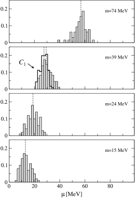
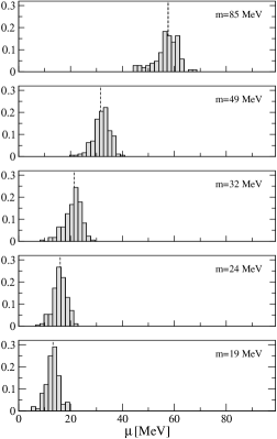
Figure 1: Normalized histograms of the spectral gap $\mu$. In the plot on the left they are obtained with the Wilson gauge and fermion action at $\beta=5.6$ on a $32\times 24^{3}$ lattice, and for bare current quark masses $m$ as reported in the plots [16]. The darker line labeled by $C_{1}$ is obtained with the very same parameters, but with a volume of $64\times 24^{3}$. The dotted vertical line is the median of the distribution. In the plot on the right there are analogous histograms for the Wilson gauge action and SW non-perturbatively improved fermions obtained at $\beta=5.3$ on a lattice $48\times 24^{3}$ [18].

At the volumes and masses considered, the distribution looks rather symmetric around the median $\overline{\mu}$, which is shifted toward smaller values when the quark mass decreases. The plots of the median versus the current quark mass shown in Fig. 2 reveal that $\overline{\mu}$ is compatible with a linear function of the mass, the slope being roughly a number of order one at these lattice spacings.

To date, the width of the distributions $\sigma$ has been studied at several volumes and masses with Wilson fermions only. Data indicate that $\sigma$ does not clearly depend on the quark mass and it scales as

$$\sigma\simeq\frac{a}{\sqrt{V}}\;,$$ (6)

$V$ being the volume in physical units. The proportionality with $a$ suggests that the width could result from short-distance fluctuations.

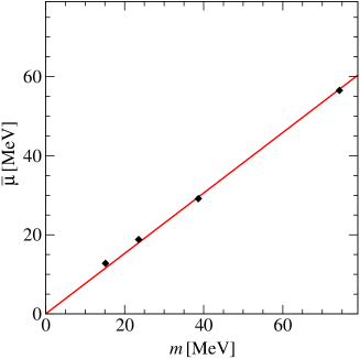
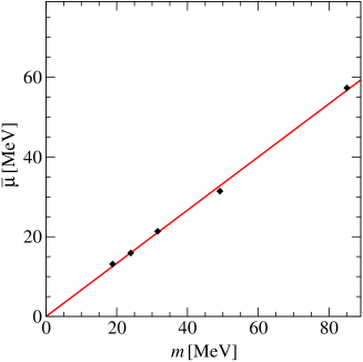
Figure 2: The median $\overline{\mu}$ of the spectral gap in MeV versus the bare current quark mass from the same numerical data as reported in Fig. 1.

An important conclusion that can be drawn from these results is that the spectrum of the Wilson operator at a given mass and for fine lattice spacings have, for practical purposes, a gap if the volume is large enough [16]. It would be more than welcome to have an analytic control on the spectral gap distribution also in this case. A first step in this direction has already been taken this year in Ref. [33]. By comparing the result in Eq. (6) with the second formula in Eq. (4), it can be noticed that the width of the distribution is much larger with Wilson fermions in the interesting ranges of parameter values. For example for $a\sim 0.072$, $L=2.4$ fm and for a lattice volume $2L\times L^{3}$, I get $\sigma\sim 1.7$ MeV, which is roughly one order of magnitude larger than the value reported in Eq. (5).

The existence of a gap in the spectrum of the Wilson–Dirac operator is also one of the reasons why the new generation of algorithms can simulate these fermions so efficiently. The range of stability where HMC algorithms can be safely applied can be defined, for instance, by requiring that $\overline{\mu}\geq 3\sigma$. By using the empirical fact that $\overline{\mu}\simeq Zm$ and $\sigma\simeq a/\sqrt{V}$, the bound can be written as

$$m\geq\frac{3\sigma}{Z}\simeq\frac{3a}{Z\sqrt{V}}\;,$$ (7)

which clearly shows the dependence of the quark mass accessible to HMC simulations from the lattice spacing and size. Since it turns out (see below) that the ratio $B=M_{\pi}^{2}/2m$ is practically independent of $m$, the previous bound can be written as

$$M_{\pi}\,L\geq\sqrt{3\sqrt{2}a\frac{B}{Z}}\;.$$ (8)

By inserting the numerical values, the condition $M_{P}L\geq 3$ is sufficient for the bound to be satisfied at $a\leq 0.09$ fm [16, 18]. A lattice with linear extension $L\simeq 2.4$ fm is more than sufficient for simulating a pion with $300$ MeV mass. Failing to fulfill the bound in Eq. (7) could lead to instabilities in the particular HMC algorithm used, which in turn could even fake the presence of a phase transition in the theory.

4 Two-flavour QCD results from the Schrödinger functional

The ALPHA collaboration is continuing the long-term program of non-perturbative renormalization of QCD [34, 35, 36]. The large-scale separation, which must be addressed, represents a formidable challenge for numerical simulations. The concept of an intermediate finite-volume renormalization scheme allows them to attack the problem on the lattice. The relation between a hadronic quantity and a suitable observable defined in the finite-volume renormalization scheme is computed at low energy [34]. The observable is then evolved non-perturbatively to higher scales using a recursive procedure [35]. Eventually the perturbative regime is reached, and the matching with perturbation theory is straightforward (for a review see Ref. [37]). The finite-volume renormalization scheme adopted is based on the Schrödinger functional (SF) ${\cal Z}$, i.e. the quantum propagation amplitude for going from some field configuration $C$ at time $x_{0}=0$ to another field configuration $C^{\prime}$ at the time $x_{0}=T$:

$${\cal Z}[C^{\prime},C]=e^{-\Gamma}=\int D[U,\psi,\bar{\psi}]\,e^{-S[U,\psi,\bar{\psi}]}\;,$$ (9)

where $C$ and $C^{\prime}$ depend on some parameters $\eta$ and $\nu$; see Ref. [38, 39] for more details. The strong-coupling constant can, for instance, be defined as [39, 40]

$${\frac{\partial\Gamma}{\partial\eta}\Big{|}_{\eta=\nu=0}=\frac{k}{\bar{g}^{2}}}\,,$$ (10)

where the normalization ${k}$ is chosen such that the tree-level value of $\bar{g}^{2}$ equals its bare value for all values of the lattice spacings.

The ALPHA collaboration has recently completed the computation of the running of the coupling constant with two massless flavours [40]. They implemented the Schrödinger functional with a simple plaquette gauge action and with SW fermions, fixing the coefficient $c_{\mathrm{SW}}$ to the value determined non-perturbatively in Ref. [20]. The small discretization errors allowed them to safely extrapolate the results to the continuum limit with moderate errors, and to obtain for the parameter $\Lambda$:

$$-\log(\Lambda\,L_{\mathrm{max}})=1.09(7)\;\;\;\;\mathrm{at}\,\;\;u_{\mathrm{max}}=\bar{g}^{2}(L_{\mathrm{max}})=5.5\,.$$ (11)

In the interval $u_{\mathrm{max}}=3.0$–$5.5$ their results can be parametrized as

$$-\log(\Lambda\,L_{\mathrm{max}})=\frac{1}{2\,b_{0}\,u_{\mathrm{max}}}+\frac{b_{1}}{2\,b_{0}^{2}}\log(b_{0}\,u_{\mathrm{max}})-0.1612+0.0379\,u_{\mathrm{max}}\;.$$ (12)

The running of the coupling in the SF scheme as a function of $\mu/\Lambda$ is shown in the first plot of Fig. 3. For $\alpha\leq 0.2$ they observe an excellent agreement with 3-loop perturbation theory, while at larger couplings the perturbative approximation becomes inadequate quite rapidly. When compared with the running in the pure Yang–Mills theory [34], a clear $N_{\mathrm{F}}$ dependence is observed. Thanks to their work, the energy dependence of the strong coupling in the SF scheme is now known over more than two orders of magnitude in two-flavour QCD.

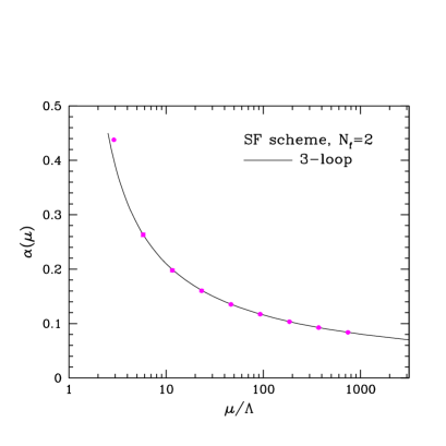
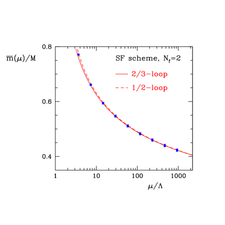
Figure 3: Running of the strong coupling constant and of the quark mass in two-flavour QCD in the Schrödinger functional scheme.

The determination of $\Lambda$ in units of a physical hadronic scale requires the computation of $L_{\mathrm{max}}$ in the same units. For lack of low-energy data, they used the Sommer scale [41] $r_{0}/a$ computed in Ref. [42] and, by assigning to it the physical value of $r_{0}=0.5$ fm, they obtain $\Lambda^{(2)}_{\overline{\mathrm{MS}}}=245(16)(16)$ MeV. In full QCD, $r_{0}$ tends to be a less convenient reference scale with respect to the quenched approximation: it requires large statistics at fine lattice spacing; it is not clear how to extrapolate its value from the simulated masses to the physical point; its physical value is not well determined since it cannot be measured directly in experiments. An important improvement in the determination of $\Lambda$ can be achieved by computing $L_{\mathrm{max}}$ in units of the pion decay constant $F_{\pi}$ or the nucleon mass. Their most recent efforts in full QCD simulations with two flavours is motivated also by this goal [43].

This year the ALPHA collaboration completed the computation of the factor that relates the running-quark mass in the Schrödinger functional scheme to the renormalization-group-invariant (RGI) one in two-flavour QCD [44]. In a mass-independent renormalization scheme, the relation between the RGI quark mass and the bare current mass is given by

$$M=Z_{M}(g_{0})\,m(g_{0})\;.$$ (13)

The computation of $Z_{M}(g_{0})$ can be split into two parts:

$$Z_{M}(g_{0})=\frac{M}{\overline{m}(\mu)}\,\frac{Z_{A}(g_{0})}{Z_{P}(g_{0},a\mu)}\;.$$ (14)

They computed the factor $M/\overline{m}(\mu)$, which is clearly regularization-independent but scheme-dependent, in the SF scheme over more than two orders of magnitude in energy, as shown in the right plot of Fig. 3. The matching factor $Z_{A}(g_{0})/Z_{P}(g_{0},a\mu)$ can be computed at low energy, and therefore no large energy differences are involved in the simulations. It is regularization- and scheme-dependent, and clearly depends also on the bare coupling. The ALPHA collaboration computed this factor in the SF scheme for the simple plaquette gauge action and for the SW non-perturbative improved fermions for a range of bare couplings [45, 44]. At this point the goal of computing the renormalized light-quark masses with controlled errors can be reached by matching these results with the computation of the bare current quark masses in large-volume simulations at light quark masses.

5 Effects of dynamical quarks in meson correlation functions

One of the effects of quark–antiquark pair production is the coupling of multiparticle meson states to fermion bilinears. If the sea-quark masses are light enough, the first higher state in two-point correlation functions is expected to be a three-meson system, with energy roughly equal to $(M_{0}+2\,M_{\pi})$, where $M_{0}$ and $M_{\pi}$ are the masses of the associated meson and of the pion made of sea quarks, respectively. It is clear that the lighter the sea-quark masses are, the smaller is the energy gap. As a consequence, the effect of the excited states should be more visible in an effective mass plot.

In Ref. [46] the UKQCD collaboration studied the stability of the effective mass fit with regard to possible contaminations from higher states. In the range of quark masses simulated, the ground-state energy that they determine with a two-exponential fit is quite stable with regard to the fit details. For the higher-state energy they find indicative values that turns out to be consistent with the expected three-meson state spectrum.

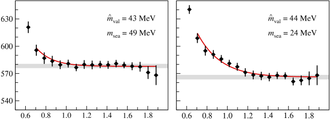
Figure 4: Results for effective pion masses $M_{\mathrm{eff}}(t)$ in MeV as a function of the time $t$ in units of fermi. They are computed with the SW non-perturbative improved action at $\beta=5.3$ on a volume of $48\times 24^{3}$ [17].

This year, much more precise results at much lighter quark masses are available [17]. Examples of effective-mass plots from the two-point function of non-singlet pseudoscalar densities are shown in Fig. 4. In the two plots the average valence-quark bare current masses $\hat{m}_{\rm val}$ and the meson masses $M_{0}$ (grey bands) are chosen to be nearly the same, while the bare sea-quark mass $m_{\rm sea}$ changes by a factor of $2$. The presence of higher-states contributions is clearly seen in the data, and a statistically significant quark-mass dependence is observed [17]. The effect of higher states becomes more pronounced when the sea-quark mass become lighter. The solid line is a fit of the form

$$M_{\mathrm{eff}}(t)=M_{0}+ce^{-2\,M_{\pi}t}+\cdots\;,$$ (15)

where $M_{0}$ and $c$ are free parameters, and $M_{\pi}$ is extracted from the pseudoscalar correlation function made of sea-quarks only. The $\chi^{2}/\mathrm{d.o.f.}$ of the fits indicates that the two-state formula in Eq. (15) is compatible with the data in the time range considered. In Ref. [17] analogous effects are also observed in the vector channels.

Apart for its own physical interest, it is quite clear that at light-quark masses the presence of multimeson states will complicate the extraction of ground-state energies from the simulated data. The computation of hadron masses may require accurate data at larger time separations than was the case in quenched QCD.

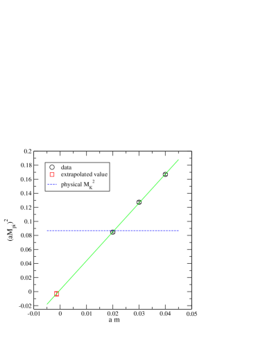
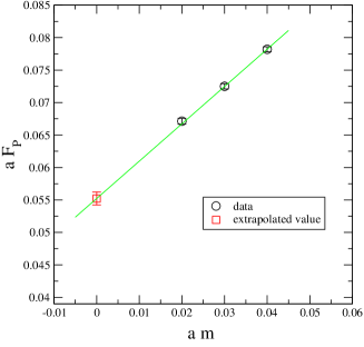
Figure 5: Quark-mass dependence of the pion mass square and decay constant computed with domain-wall fermions on a volume $32\times 16^{3}$, with a lattice spacing of $a\sim 0.12$ fm [47].

6 Pseudoscalar meson masses and decay constants from two-flavour simulations

In the recent past, pion masses and decay constants were computed in two-flavour QCD at quark masses $m\geq m_{s}/2$ by several collaborations [2, 5, 4, 6, 46, 47]. Data from Ref. [47] generated with domain-wall fermions on lattices of size $32\times 16^{3}$ with a lattice spacing of $a\sim 0.12$ fm are shown in Fig. 5. Be it for the pion mass square or for the decay constant, they find a remarkable linear behaviour in the range $(m_{s}/2)$–$m_{s}$. Similar results have been obtained by the other collaborations with different gluon and fermions actions. After this experience with two-flavour QCD, the RBC and the UKQCD collaborations decided to move on and simulate $2+1$ flavours with domain-wall fermions. The first preliminary results have already been presented at this conference. The reader can find details of these simulations in their talks [48, 49, 50, 51]. The PACS-CS collaboration is working hard to implement a combination of DD-HMC and PHMC algorithms to simulate QCD with $2+1$ flavours with the SW non-perturbative improved fermions and with light up and down quark masses. The first experience of this remarkable effort have already been reported at this conference in Refs. [52, 53, 54]

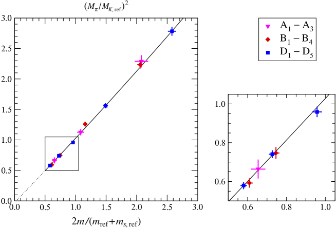
	Lat	$k$	$N_{\mathrm{trj}}$	$N_{\mathrm{conf}}$
W/W	$A_{1}$	0.15750	6400	64
$V\,a^{-4}=32\times 24^{3}$	$A_{2}$	0.15800	10900	109
$\beta=5.6$	$A_{3}$	0.15825	10000	100
W/W	$B_{1}$	0.15410	5000	100
$V\,a^{-4}=64\times 32^{3}$	$B_{2}$	0.15440	5050	101
$\beta=5.8$	$B_{3}$	0.15455	5200	104
	$B_{4}$	0.15462	5100	102

	Lat	$k$	$N_{\mathrm{trj}}$	$N_{\mathrm{conf}}$
W/SW	$D_{1}$	0.13550	5200	104
$V\,a^{-4}=48\times 24^{3}$	$D_{2}$	0.13590	5130	171
$\beta=5.3$	$D_{3}$	0.13610	5040	168
	$D_{4}$	0.13620	5040	168
	$D_{5}$	0.13625	5040	169

Figure 6: Parameters of the lattices generated in Refs. [17, 18] with the Wilson gauge action and Wilson ($W/W$) and SW non-perturbative improved ($W/SW$) fermions are given in the tables. $k$ is the hopping parameter, $N_{\mathrm{trj}}$ is the number of HMC trajectories generated after thermalization, and $N_{\mathrm{conf}}$ is the number of independent configurations selected to compute the observables. The dependence of the square of the pion mass $M_{\pi}$ on the sea-quark current mass $m$ in units of the same quantities at the reference point is shown in the plots. The solid curve is a quadratic least-squares fit (with constant term) of all data points. The plot on the right is a blow up of the region enclosed by the little box.

This year for the first time we have a quite large amount of results obtained in two-flavour QCD at quark masses as low as $(m_{s}/5)$–$(m_{s}/4)$. The richest set of data has been accumulated with the DD-HMC algorithm in Refs. [17, 18]. Tables with the actions implemented, lattice parameters, and number of configurations generated are shown in Fig. 6. The authors supplement the two-flavour theory with a quenched strange quark. They define the reference point to be where the mass of the $\pi$, $K$ and $K^{*}$ mesons satisfy

$$\frac{M_{K,\mathrm{ref}}}{M_{K^{*},\mathrm{ref}}}=0.554\,\qquad\qquad\frac{M_{\pi,\mathrm{ref}}}{M_{K,\mathrm{ref}}}=0.85\;.$$ (16)

The lattice spacing $a$ is then fixed by setting the value $M_{K,\mathrm{ref}}=495$ MeV [17]. This procedure extends similar ideas already implemented in the quenched approximation [55, 56]. For the three sets of lattices $A$, $B$ and $C$ (see table in Fig. 6) they obtain $a=0.0717(15)$, $0.0521(7)$ and $0.0784(10)$, respectively. These values are significantly smaller that those reported in Ref. [57], determined by fixing $a$ from the Sommer scale. As a consequence the pion and the quark masses in physical units quoted here are significantly larger than in Ref. [57].

	$a\mu$	$N_{\mathrm{trj}}$
tlSym/tm	0.0150	5000
$V\,a^{-4}=48\times 24^{3}$	0.0100	5000
$\beta=3.90$	0.0064	5000
	0.0040	5000
tlSym/tm	0.0060	500
$V\,a^{-4}=64\times 32^{3}$	0.0030	2200
$\beta=4.05$

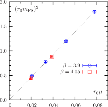
Figure 7: Current status of the simulations with the tree-level Symanzik improved gauge action (tlSym) and twisted-mass fermions at maximal twist reported in Ref. [24]. The bare quark mass $a\mu$ and the number of trajectories generated after thermalization are listed in the table. The dependence of the square of the pion mass $M_{\pi}$ on the sea-quark twisted mass $\mu$ is shown in the plot. Masses are expressed in units of $r_{0}$ computed at the lightest simulation point.

Once the lattice is calibrated, results from the various sets of simulations can be compared. In Fig. 6 the ratio $(M_{\pi}/M_{K,\mathrm{ref}})^{2}$ is shown as a function of the corresponding ratio of current quark masses. The plots reveal several remarkable properties of the results. Data generated with two different discretizations and three lattice spacings lie on the same “universal” curve within the statistical fluctuations. This supports the fact that the discretization effects in the relation between the pseudoscalar-meson-mass squared and the current quark mass are small. This fact could be explained with the observation that $O(a)$ effects are absent at leading order in chiral perturbation theory if the current quark mass is used [58]. The second remarkable property is the linear behaviour of the data over such a wide range of quark masses. There is a visible curvature towards the larger masses, but the coefficient of the quadratic term in the empirical fit (solid line) is small. Moreover in the range $(M_{\pi}/M_{K,\mathrm{ref}})\leq 1.1$, the results are well represented by a straight line through the origin.

This year the QCDSF-UKQCD collaboration supplemented their set of data generated with the SW non-perturbative improved action at $\beta=5.29$ with two new points with quark masses well below $m_{s}/2$ [23, 59]. Even though they are based on a still limited statistics, their findings for $M_{\pi}^{2}$ are compatible with the previous observations. The ETM collaboration is simulating two-flavour QCD with the tree-level Symanzik improved gauge action (tlSym) and twisted-mass fermions at maximal twist. At this conference they presented data at fine lattices and small quark masses [24]. A summary of the parameters of their simulations and of their results for the pseudoscalar mass square are reported and shown in Fig. 7. The value of $r_{0}$ used to plot the data is the one obtained at their lightest simulation point. Data collected so far are well compatible with a linear behaviour of $M_{\pi}^{2}$ versus the quark mass.

Data generated in Refs. [17, 18] for pion decay constant $F_{\pi}$ are shown in Fig. 8. All data sets are statistically compatible with a linear behaviour in the range of mass explored. The results of the $D$ lattices turn out to be quite different from those of the $A$ and $B$ lattices. Although the two lines are visibly different, the fitted values of their slopes, $0.235(11)$ and $0.192(11)$, deviate from each other by less than $3$ times the combined statistical error. The statistical significance of the effect is thus not conclusive. A similar linear behaviour in $F_{\pi}$ has been observed also in the data of the ETM collaboration [24].

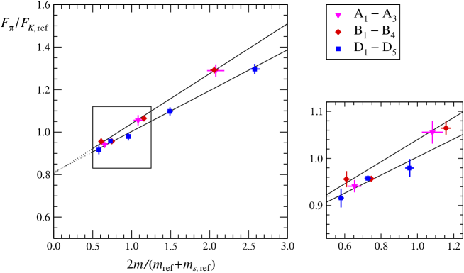
Figure 8: Dependence of the pion decay constant $F_{\pi}$ on the sea-quark mass $m$ in units of the same quantities at the reference point as obtained in Ref. [17, 18]. The solid curves are linear fits of the data points from the $A$ and $B$ lattices (upper line) and of the points from the $D$ lattices (lower line).The plot on the right is a blow up of the region enclosed by the little box.

7 Finite-volume corrections for pseudoscalar meson masses

Finite-volume effects are expected to be negligible in hadron masses if the linear extension $L$ of the lattice is much larger than the cloud of virtual particles surrounding them. In this regime of volumes, i.e. $FL\gg 1$ and $M_{\pi}L\gg 1$, the leading finite-volume corrections to pion masses can be estimated in ChPT. At the next-to-leading order (NLO) [60, 61, 62]

$$M_{\pi}^{2}(L)=M_{\pi}^{2}\left\{1+\frac{1}{2}\frac{M^{2}}{(4\pi F)^{2}}\,g_{1}(M)\right\}$$ (17)

where

$$g_{1}(M)=4\sum_{\{n_{k}\}}\,\!\!\!^{\prime}\frac{1}{M|q_{n}|}K_{1}(|q_{n}|M)\;.$$ (18)

$M^{2}=2\,B\overline{m}$ is the pion mass at leading order, $B$ and $F$ are the leading-order low-energy constants, $\sum_{\{n_{k}\}}\,\!\!\!\!\!\!\!\!\!\!\!\!\!\!\!^{\prime}\;\;\;\;$ denotes the sum over all three-dimensional vectors of integers with the exception of $n=(0,0,0)$, $q_{n}^{2}=\sum_{k=1}^{3}(n_{k}L)^{2}$, and $K_{1}$ is a modified Bessel function. These corrections are exponentially small in $M_{\pi}L$, i.e. the leading exponential in Eq. (17) is given by

$$\frac{M_{\pi}(L)-M_{\pi}}{M_{\pi}}=\displaystyle\frac{M^{2}}{(4\pi F)^{2}}{\frac{3\sqrt{2\pi}}{(ML)^{3/2}}e^{-ML}}\;.$$ (19)

Once the (infinite) volume values of $F_{\pi}$ and $M_{\pi}$ are known, Eq. (17) gives a parameter-free and model-independent estimate of the leading corrections at asymptotically large volumes. An analogous formula can be written for the decay constant. Whether this regime has been reached for the lattices currently simulated in two-flavour QCD still needs to be confirmed. Other effects such as the squeezing of the meson wave function [63] cannot be taken into account in ChPT, where the pion is a “point-like” particle, and therefore we do not have any analytic handle on them.

Thanks to their universality, finite-size effects can be estimated by simulating lattices with different volumes at a single (fine) lattice spacing. Discretization effects add small corrections, which can be neglected to a first approximation. A careful study for the pion mass has been carried out in Ref. [64]. This year their data can be supplemented by the results from Refs. [13, 18], generated with the same simple-plaquette gluon action and with Wilson fermions at the very same mass. The values of pion masses at volumes that satisfy the stability bound in Section 3 are reported in the table of Fig. 9.

$\beta$	$K$	$T\times L^{3}$	$aM_{\pi}(L)$	$M_{\pi}L$	Ref.
5.6	0.1575	$32\times 12^{3}$	0.3576(89)	3.31(2)	[64]
		$32\times 14^{3}$	0.3048(44)	3.86(3)	[64]
		$32\times 16^{3}$	0.2806(35)	4.41(3)	[64]
		$40\times 24^{3}$	0.2765(26)	6.61(4)	[64]
		$32\times 24^{3}$	0.2744(21)	6.61(4)	[18]
5.6	0.1580	$32\times 16^{3}$	0.233(5)	3.15(3)	[64]
		$32\times 16^{3}$	0.242(4)	3.15(3)	[13]
		$40\times 24^{3}$	0.1991(33)	4.73(4)	[64]
		$32\times 24^{3}$	0.1969(16)	4.73(4)	[18]

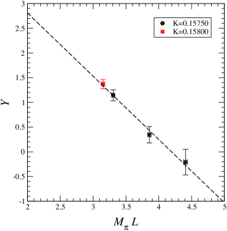
Figure 9: Meson masses computed with the simple plaquette gauge action and Wilson fermions at $\beta=5.6$ for various lattice sizes. The value of $(a\,M_{\pi})$ is obtained by combining data at the largest spatial volume. In the plot the quantity $Y$, defined in Eq. (20), is shown as a function of $M_{\pi}L$. The dashed line is a linear fit to the data points.

To compare the ChPT prediction in Eq. (17) with numerical data, I make the working assumption that finite-volume corrections at the largest volumes are negligible within the statistical errors. This assumption is compatible with Eq. (17). In Fig. 9 the quantity

$$Y=\log\left[\displaystyle\frac{M_{\pi}(L)-M_{\pi}}{M_{\pi}}\times\frac{(M_{\pi}L)^{3/2}}{3\sqrt{2\pi}(aM_{\pi})^{2}}\right]$$ (20)

is shown in logarithmic scale as a function of $M_{\pi}L$. The linearity of the data agrees well with an exponential behaviour of the form $e^{-M_{\pi}L}$. The NLO ChPT correction in Eq. (17), however, underestimates the pre-factor by roughly one order of magnitude at these volumes and quark masses. This means that a volume with a linear extension of $L\sim 1.2$ fm is far too small for ChPT to apply. Even though we do not have a quantitative explanation for it, the mismatch between the data and ChPT is not unexpected [63]. In such a small volume the pion wave-function is most likely modified significantly, and treating the pion as a point-like particle is an approximation too crude. What is maybe more important in this regard is to find the lattice sizes where finite-volume effects at the masses currently simulated match the asymptotic correction expected in the chiral effective theory, or where these corrections are negligible with respect to the statistical errors. This is the minimal requirement for the data to be useful, and eventually for being compared with ChPT. It is most likely that this goal can be reached in the very near future. Similar considerations apply to $F_{\pi}$.

8 Two-flavour QCD at fixed topology

This year the JLQCD collaboration started an ambitious project of simulating two-flavour QCD with Neuberger’s fermions at fixed topology [65, 66, 67, 30]. The global topological charge is frozen by supplementing the Iwasaki gluon action with the extra Boltzmann weight in the functional integral

$$\frac{\mathrm{det}\;H^{2}_{\mathrm{W}}}{\mathrm{det}\,(H^{2}_{\mathrm{W}}+\mu^{2})}\;,$$ (21)

where $H_{\mathrm{W}}$ is the Hermitian–Wilson operator with a large negative mass, and $\mu$ is a real parameter [68]. This is equivalent to introducing two additional flavours of Wilson fermions with unphysical large negative mass, and two additional twisted-mass ghosts with large mass $\mu$. Since these extra fields have masses of the order of the cut-off, they modify the theory in the ultraviolet only, and thus become irrelevant in the continuum limit. For the light physical quarks, JLQCD chooses to work with Neuberger fermions [69]. Earlier studies in the quenched approximation showed that this modified gluon action prevents the near-zero modes of $H_{\mathrm{W}}$ from reaching zero [68]. It thus fixes the global topological charge as defined via the index of the corresponding Neuberger operator. In this way data at fixed topology can be generated efficiently: the topological charge does not have to be computed for each configuration, and only those with the desired topology are produced. An important technical advantage is that the discontinuities that appear in the HMC Hamiltonian when a near-zero mode of $H_{\mathrm{W}}$ passes through zero are avoided. Simulations with a plain HMC algorithm are thus feasible. The cluster decomposition property of the underlying local quantum field theory suggests that fixing the global topological charge should have harmless effects on physical observables at asymptotically large volumes. However, unlike what happens in the full theory, the suppression of finite-size effects should be power-like in $L$ rather than exponential. At the volumes accessible so far in numerical simulations, these effects can be relevant and a careful analysis of them is needed.

	$am$	$N_{\mathrm{trj}}$
	0.100	3590
$IW^{*}/N$	0.070	3500
$\beta=2.30$	0.050	3500
$Va^{-4}=32\times 16^{3}$	0.035	4150
$\mu=0.2$	0.025	4320
$\nu=0$	0.015	2150

Figure 10: The table shows the lattice parameters of the main JLQCD simulations with the Iwasaki gluon action, with the extra weight defined in Eq. (21), and Neuberger’s fermions ($IW^{*}/N$): $am$ is the bare quark mass and $N_{\mathrm{trj}}$ is the number of trajectories generated. The plot represents the quark-mass dependence of the pion mass square; the dashed line is a linear fit of the data.

The JLQCD collaboration generates the gauge configurations with the Hasenbusch-accelerated HMC algorithm with multiple-time scale integration [66]. The lattice volume is $32\times 16^{3}$, $\beta=2.30$ and so far the topological charge is $\nu=0$. With this set-up they expect to have a lattice spacing of roughly $0.12$ fm and a linear size extent of $L\sim 1.9$ fm. The list of bare quark masses considered is given in the table of Fig. 10. They should be in the range $(m_{s}/6)$–$m_{s}$. The first preliminary results that JLQCD has obtained for the pion mass squared are shown in the plot of Fig. 10 as a function of the bare quark mass. Also in their data a remarkable linear behaviour is observed with no statistically significant deviation from a simple linear fit (dashed line). Before drawing any physics conclusions from these preliminary results, more simulations at several volumes and topologies are needed for a careful study of finite-size effects [67].

JLQCD performed also a test run in the $\epsilon$-regime of QCD, on a lattice of $32\times 16^{3}$, $\beta=2.35$ and $am=0.002$. The statistics accumulated is still limited to $1400$ trajectories, but preliminary results for ratios of eigenvalues and pseudoscalar correlation functions were already presented in Ref. [30]. A comparison with random-matrix-theory predictions is shown in Fig. 11. The $N_{\mathrm{F}}$ dependence of the data is compatible with the expectations of random-matrix theory within the large statistical errors. Also in this case are needed larger statistical samples before drawing any firm conclusion.

9 Chiral perturbation theory confronts lattice data

At the NLO in the chiral expansion of the two-flavour theory, the quark-mass dependence of the pseudoscalar meson mass and decay constant is given by

$$\begin{array}[]{lcl}M^{2}_{\pi}&=&\displaystyle M^{2}\,\Big{\{}1+\frac{M^{2}}{32\pi^{2}F^{2}}\log\left(\frac{M^{2}}{\Lambda_{3}^{2}}\right)+\dots\Big{\}}\\[14.22636pt] F_{\pi}&=&\displaystyle\;\;F\;\Big{\{}1-\frac{M^{2}}{16\pi^{2}F^{2}}\log\left(\frac{M^{2}}{\Lambda_{4}^{2}}\right)\;+\;\dots\Big{\}}\;.\end{array}$$ (22)

Following the convention introduced in Ref. [70], we can define the NLO low-energy constants as

$${\bar{l}_{3}}={\displaystyle\log\left(\frac{\Lambda^{2}_{3}}{M^{2}}\right)\Big{|}_{M=139.6\mathrm{MeV}}}\;,\qquad\qquad{\bar{l}_{4}}={\displaystyle\log\left(\frac{\Lambda^{2}_{4}}{M^{2}}\right)\Big{|}_{M=139.6\mathrm{MeV}}}\,.$$ (23)

They can be determined, at least in principle, by matching lattice QCD results with the formulas in Eqs. (22).

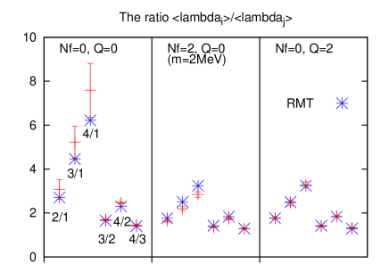
Figure 11: Ratios of low-lying eigenvalues $\lambda_{i}/\lambda_{j}$ (denoted by “$i/j$”) of the Neuberger operator for $(N_{\mathrm{F}},Q)=(0,0)$, $(2,0)$, $(0,2)$ (crosses). The random-matrix-theory predictions are also indicated (stars).

Data available to date do not allow for a determination of these low-energy constants with a reliable estimate of the errors. Nevertheless it is interesting to look in some detail into the analysis presented in Ref. [17], which is based on the richest set of data at light-quark masses in the two-flavour theory. The reference point introduced in Section 6 is a useful idea in this context. The dimensionful quantities expressed in units of the scales at the reference point are free from systematics coming from the determinations of the lattice spacing and of ultraviolet renormalization constants. Following Ref. [17], we can introduce

$$x=\frac{2\,m}{m_{\mathrm{ref}}+m_{s,\mathrm{ref}}}\;,\qquad\qquad C=\frac{M_{K,\mathrm{ref}}^{2}}{32\pi^{2}F_{K,\mathrm{ref}}^{2}},$$ (24)

and if we define

$$\hat{F}=\frac{F}{F_{K,\mathrm{ref}}},\qquad\hat{B}=\frac{m_{\mathrm{ref}}+m_{s,\mathrm{ref}}}{M_{K,\mathrm{ref}}^{2}}\,B\,,\qquad\hat{l}_{n}=\log\left(\frac{\Lambda^{2}_{n}}{M_{K,\mathrm{ref}}^{2}}\right)\,,$$ (25)

then $\hat{l}_{n}=\bar{l}_{n}-2.53$, and Eqs. (22) become

$$\begin{array}[]{lcl}\displaystyle\frac{M^{2}_{\pi}}{M^{2}_{K,\mathrm{ref}}}&=&\displaystyle\hat{B}\,x+C\frac{\hat{B}^{2}x^{2}}{\hat{F}^{2}}\left\{\log(\hat{B}\,x)-\hat{l}_{3}\right\}+\dots\\[14.22636pt] \displaystyle\frac{F_{\pi}}{F_{K,\mathrm{ref}}}&=&\displaystyle\hat{F}-2\,C\,\frac{\hat{B}\,x}{\hat{F}}\left\{\log(\hat{B}\,x)-\hat{l}_{4}\right\}+\dots\end{array}$$ (26)

In the range $M_{\pi}/M_{K,\mathrm{ref}}\leq 1.1$, the first formula in Eqs. (26) fits the data for the pion mass very well, the fit parameters being $\hat{B}=1.11(6)(3)$ and $\hat{l}_{3}=0.5(5)(1)$ (equivalently $\bar{l}_{3}=3.0(5)(1)$), where the second errors are estimates of the systematic uncertainty arising from the inaccurately known values of $C$ and $\hat{F}$; see Ref. [17] for details. The results of the fit superimposed on the simulated data is shown in the first plot of Fig. 12. No attempt has been made to estimate the systematics uncertainty coming from higher orders in ChPT, due to discretization effects or finite-volume corrections. As described at length in Sections 6 and 7, discretization effects seems to be moderate for this quantity, while a reliable check of finite-volume effects is still missing and will require simulations at larger volumes.

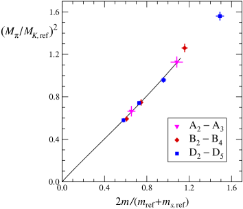
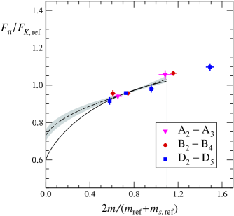
Figure 12: The pion mass $M_{\pi}$ (left) and the pion decay constant $F_{\pi}$ (right) as a function of the bare current quark mass in units of the same quantities at the reference point from Ref. [17]. The solid lines are fits in the range $M_{\pi}/M_{K,\mathrm{ref}}\leq 1.1$. using the one-loop formulas in Eqs. (26). The grey band on the right-hand plot is from a fit where a hypothetical next-order term has been included (see text).

A phenomenological analysis of low-energy experimental data gives $\bar{l}_{3}=2.9\pm 2.4$ [70, 71]. Strictly speaking, the comparison of this value with the one extracted from two-flavour lattice simulations only allows for an estimate of the contribution to this low-energy constant due to dynamical strange and charm quarks, assuming that QCD reproduces the experimental data. In practice, however, the comparison shows the potentiality of lattice QCD for the determination of $\bar{l}_{3}$ in the two-flavour theory.

The fit of the data (solid line) for the pseudoscalar decay constant with the second of Eqs. (26) is shown in the second plot of Fig. 12. The $\chi^{2}/\mathrm{d.o.f.}$ turns out to be quite good, but the absence of curvature in the data forces the extrapolated value to be quite lower than the simulated data. A more realistic fit (dashed line) can be obtained by including a hypothetical two-loop term proportional to $\hat{B}^{2}x^{2}/\hat{F}^{3}$ in the second of Eqs. (26), with a reasonable value of the coefficient $C^{\prime}=0.046$. The fit parameters $\hat{F}$ and $\hat{l}_{4}$ change from $0.60(4)$ and $1.6(1)$ to $0.73(3)$ and $0.73(8)$, respectively, when the two-loop term is added [17]. This analysis shows that data at significantly smaller quark masses, with small systematic and statistical errors, will be required for a reliable determination of the parameters in the chiral Lagrangian.

10 Conclusions

Thanks to algorithmic and technical progress achieved over the last couple of years, it is now possible to simulate QCD with dynamical quarks much more efficiently than was possible before. As a result lattices with pions as light as 250–300 MeV can be simulated with the present generation of computers.

Two-flavour QCD is already being simulated with quark masses as light as $(m_{s}/5)$–$(m_{s}/4)$ with several gluon and fermion discretizations, on quite large volumes and fine lattice spacings. Unquenched effects are clearly seen in various correlation functions. Maybe to date the most striking result is the observed linearity of the pion mass squared as a function of the current quark mass in the range $(m_{s}/4)$–$m_{s}$. Data at several (fine) lattice spacings and with several gluon and fermion actions are consistent with this picture. Finite-volume effects are still a concern. A matching of the chiral pertubation theory prediction with the finite-size effects observed in $M_{\pi}$ is still missing. In this respect simulations at several volumes are still needed. JLQCD started an ambitious project of simulating two-flavour QCD at fixed topology with exact chiral symmetry. First preliminary results of these efforts have been already presented at this conference.

Several collaborations are already simulating QCD with $2+1$ flavours. The RBC and the UKQCD collaborations are attacking the problem with domain-wall fermions, while the PACS-CS collaboration is working hard to implement a combination of DD-HMC and PHMC algorithms to simulate SW non-perturbative improved fermions.

Thanks to all this work, our community has now the possibility to perform many computations which we were dreaming about only few years ago.

Acknowledegments

Many thanks to L. Del Debbio, M. Lüscher, R. Petronzio and N. Tantalo for allowing me to present our results before their publication in Refs. [17, 18]. I warmly thank M. Lüscher for many suggestions and endless discussions during the preparation of the talk, and for a critical reading of this report. It is a pleasure to thank T. Blum, H. Fukaya, S. Hashimoto, K. Jansen, T. Kaneko, C. B. Lang, M. Lin, M. Okamoto and A. Shindler for sending their results and for interesting discussions about their work. An informative e-mail exchange with S. Sharpe about the content of our talks is acknowledged. Many thanks to the organizers for their great work in organizing the conference, and for inviting me to present this talk.

References

- [1] CP-PACS Collaboration, S. Aoki et al., Light hadron spectrum and quark masses from quenched lattice QCD, Phys. Rev. D67 (2003) 034503, [hep-lat/0206009].
- [2] TXL Collaboration, N. Eicker et al., Light and strange hadron spectroscopy with dynamical Wilson fermions, Phys. Rev. D59 (1999) 014509, [hep-lat/9806027].
- [3] T. Lippert et al., SESAM and TL results for Wilson action: A status report, Nucl. Phys. Proc. Suppl. 60A (1998) 311–334, [hep-lat/9707004].
- [4] UKQCD Collaboration, C. R. Allton et al., Effects of non-perturbatively improved dynamical fermions in QCD at fixed lattice spacing, Phys. Rev. D65 (2002) 054502, [hep-lat/0107021].
- [5] CP-PACS Collaboration, A. Ali Khan et al., Light hadron spectroscopy with two flavors of dynamical quarks on the lattice, Phys. Rev. D65 (2002) 054505, Erratum–ibid. D67 (2003) 059901, [hep-lat/0105015].
- [6] JLQCD Collaboration, S. Aoki et al., Light hadron spectroscopy with two flavors of -improved dynamical quarks, Phys. Rev. D68 (2003) 054502, [hep-lat/0212039].
- [7] S. Duane, A. D. Kennedy, B. J. Pendleton, and D. Roweth, Hybrid Monte Carlo, Phys. Lett. B195 (1987) 216–222.
- [8] C. Bernard et al., Panel discussion on the cost of dynamical quark simulations, Nucl. Phys. Proc. Suppl. 106 (2002) 199–205.
- [9] C. W. Bernard et al., The QCD spectrum with three quark flavors, Phys. Rev. D64 (2001) 054506, [hep-lat/0104002].
- [10] S. R. Sharpe, Rooted staggered fermions: good, bad or ugly?, hep-lat/0610094.
- [11] M. Lüscher, Lattice QCD and the Schwarz alternating procedure, JHEP 05 (2003) 052, [hep-lat/0304007].
- [12] M. Lüscher, Solution of the Dirac equation in lattice QCD using a domain decomposition method, Comput. Phys. Commun. 156 (2004) 209–220, [hep-lat/0310048].
- [13] M. Lüscher, Schwarz-preconditioned HMC algorithm for two-flavour lattice QCD, Comput. Phys. Commun. 165 (2005) 199–220, [hep-lat/0409106].
- [14] M. Hasenbusch, Speeding up the hybrid-Monte-Carlo algorithm for dynamical fermions, Phys. Lett. B519 (2001) 177–182, [hep-lat/0107019].
- [15] C. Urbach, K. Jansen, A. Shindler, and U. Wenger, HMC algorithm with multiple time scale integration and mass preconditioning, Comput. Phys. Commun. 174 (2006) 87–98, [hep-lat/0506011].
- [16] L. Del Debbio, L. Giusti, M. Lüscher, R. Petronzio, and N. Tantalo, Stability of lattice QCD simulations and the thermodynamic limit, JHEP 02 (2006) 011, [hep-lat/0512021].
- [17] L. Del Debbio, L. Giusti, M. Lüscher, R. Petronzio, and N. Tantalo, QCD with light Wilson quarks on fine lattices (I): first experiences and physics results, hep-lat/0610059.
- [18] L. Del Debbio, L. Giusti, M. Lüscher, R. Petronzio, and N. Tantalo, QCD with light Wilson quarks on fine lattices (II): DD-HMC simulations and data analysis, to appear.
- [19] B. Sheikholeslami and R. Wohlert, Improved continuum limit lattice action for QCD with Wilson fermions, Nucl. Phys. B259 (1985) 572.
- [20] ALPHA Collaboration, K. Jansen and R. Sommer, improvement of lattice QCD with two flavors of Wilson quarks, Nucl. Phys. B530 (1998) 185–203, Erratum–ibid B643 (2002) 517–518, [hep-lat/9803017].
- [21] CP-PACS and JLQCD Collaboration, A. Ukawa, Computational cost of full QCD simulations experienced by CP-PACS and JLQCD collaborations, Nucl. Phys. Proc. Suppl. 106 (2002) 195–196.
- [22] J. C. Sexton and D. H. Weingarten, Hamiltonian evolution for the hybrid Monte Carlo algorithm, Nucl. Phys. B380 (1992) 665–678.
- [23] M. Göckeler et al., Simulating at realistic quark masses: pseudoscalar decay constants and chiral logarithms, hep-lat/0610066.
- [24] ETM Collaboration, K. Jansen and C. Urbach, First results with two light flavours of quarks with maximally twisted mass, hep-lat/0610015.
- [25] M. A. Clark and A. D. Kennedy, Accelerating dynamical fermion computations using the rational hybrid Monte Carlo (RHMC) algorithm with multiple pseudofermion fields, hep-lat/0608015.
- [26] M. A. Clark, The rational hybrid Monte Carlo algorithm, hep-lat/0610048.
- [27] F. Niedermayer, Exact chiral symmetry, topological charge and related topics, Nucl. Phys. Proc. Suppl. 73 (1999) 105–119, [hep-lat/9810026].
- [28] T. Wilke, T. Guhr, and T. Wettig, The microscopic spectrum of the QCD Dirac operator with finite quark masses, Phys. Rev. D57 (1998) 6486–6495, [hep-th/9711057].
- [29] L. Giusti, M. Lüscher, P. Weisz, and H. Wittig, Lattice QCD in the epsilon-regime and random matrix theory, JHEP 11 (2003) 023, [hep-lat/0309189].
- [30] JLQCD Collaboration, H. Fukaya et al., Dynamical overlap fermions in the epsilon-regime, hep-lat/0610024.
- [31] S. Aoki, New phase structure for lattice QCD with Wilson fermions, Phys. Rev. D30 (1984) 2653.
- [32] ALPHA Collaboration, R. Frezzotti, P. A. Grassi, S. Sint, and P. Weisz, Lattice QCD with a chirally twisted mass term, JHEP 08 (2001) 058, [hep-lat/0101001].
- [33] S. R. Sharpe, Discretization errors in the spectrum of the Hermitian Wilson-Dirac operator, Phys. Rev. D74 (2006) 014512, [hep-lat/0606002].
- [34] M. Lüscher, R. Narayanan, P. Weisz, and U. Wolff, The Schrödinger functional: A renormalizable probe for non abelian gauge theories, Nucl. Phys. B384 (1992) 168–228, [hep-lat/9207009].
- [35] M. Lüscher, P. Weisz, and U. Wolff, A numerical method to compute the running coupling in asymptotically free theories, Nucl. Phys. B359 (1991) 221–243.
- [36] K. Jansen et al., Non-perturbative renormalization of lattice QCD at all scales, Phys. Lett. B372 (1996) 275–282, [hep-lat/9512009].
- [37] M. Lüscher, Advanced lattice QCD, in: Probing the Standard Model of Particle Interactions (Les Houches 1997), Eds. R. Gupta et al. (Elsevier, Amsterdam, 1999), hep-lat/9802029.
- [38] M. Lüscher, R. Sommer, U. Wolff, and P. Weisz, Computation of the running coupling in the SU(2) Yang-Mills theory, Nucl. Phys. B389 (1993) 247–264, [hep-lat/9207010].
- [39] M. Lüscher, R. Sommer, P. Weisz, and U. Wolff, A precise determination of the running coupling in the SU(3) Yang-Mills theory, Nucl. Phys. B413 (1994) 481–502, [hep-lat/9309005].
- [40] ALPHA Collaboration, M. Della Morte et al., Computation of the strong coupling in QCD with two dynamical flavours, Nucl. Phys. B713 (2005) 378–406, [hep-lat/0411025].
- [41] R. Sommer, A new way to set the energy scale in lattice gauge theories and its applications to the static force and in SU(2) Yang-Mills theory, Nucl. Phys. B411 (1994) 839–854, [hep-lat/9310022].
- [42] QCDSF Collaboration, M. Göckeler et al., Determination of light and strange quark masses from full lattice QCD, Phys. Lett. B639 (2006) 307–311, [hep-ph/0409312].
- [43] H. B. Meyer et al., Exploring the HMC trajectory-length dependence of autocorrelation times in lattice QCD, hep-lat/0606004.
- [44] ALPHA Collaboration, M. Della Morte et al., Non-perturbative quark mass renormalization in two-flavor QCD, Nucl. Phys. B729 (2005) 117–134, [hep-lat/0507035].
- [45] M. Della Morte, R. Hoffmann, F. Knechtli, R. Sommer, and U. Wolff, Non-perturbative renormalization of the axial current with dynamical Wilson fermions, JHEP 07 (2005) 007, [hep-lat/0505026].
- [46] UKQCD Collaboration, C. R. Allton et al., Improved Wilson QCD simulations with light quark masses, Phys. Rev. D70 (2004) 014501, [hep-lat/0403007].
- [47] Y. Aoki et al., Lattice QCD with two dynamical flavors of domain wall fermions, Phys. Rev. D72 (2005) 114505, [hep-lat/0411006].
- [48] RBC and UKQCD Collaboration, R. Mawhinney et al., Production and properties of flavor DWF ensembles, these proceedings.
- [49] RBC and UKQCD Collaboration, C. Maynard et al., Baryon spectrum in flavour domain wall QCD from QCDOC, these proceedings.
- [50] RBC and UKQCD Collaboration, M. Lin et al., Chiral extrapolations in flavor domain wall fernions simulations, these proceedings.
- [51] RBC and UKQCD Collaboration, C. Allton et al., Light meson masses and non-perturbative renormalisation in 2+1 flavour domain wall qcd, hep-lat/0610119.
- [52] PACS-CS Collaboration, A. Ukawa et al., Status and physics plan of the PACS-CS project, PoS LAT2006 (2006) 039.
- [53] PACS-CS Collaboration, K.-I. Ishikawa et al., An application of the UV-filtering preconditioner to the polynomial hybrid Monte Carlo algorithm, hep-lat/0610037.
- [54] PACS-CS Collaboration, Y. Kuramashi et al., 2+1 flavor lattice QCD with Lüscher’s domain-decomposed HMC algorithm, hep-lat/0610063.
- [55] C. R. Allton, V. Gimenez, L. Giusti, and F. Rapuano, Light quenched hadron spectrum and decay constants on different lattices, Nucl. Phys. B489 (1997) 427–452, [hep-lat/9611021].
- [56] ALPHA Collaboration, J. Heitger, R. Sommer, and H. Wittig, Effective chiral lagrangians and lattice QCD, Nucl. Phys. B588 (2000) 377–399, [hep-lat/0006026].
- [57] M. Lüscher, Lattice QCD with light Wilson quarks, PoS LAT2005 (2006) 002, [hep-lat/0509152].
- [58] S. R. Sharpe and R. L. Singleton, Spontaneous flavor and parity breaking with Wilson fermions, Phys. Rev. D58 (1998) 074501, [hep-lat/9804028].
- [59] M. Göckeler et al., Simulating at realistic quark masses: light quark masses, hep-lat/0610071.
- [60] J. Gasser and H. Leutwyler, Light quarks at low temperatures, Phys. Lett. B184 (1987) 83.
- [61] J. Gasser and H. Leutwyler, Thermodynamics of chiral symmetry, Phys. Lett. B188 (1987) 477.
- [62] J. Gasser and H. Leutwyler, Spontaneously broken symmetries: effective lagrangians at finite volume, Nucl. Phys. B307 (1988) 763.
- [63] M. Fukugita, H. Mino, M. Okawa, G. Parisi, and A. Ukawa, Finite size effect for hadron masses in lattice QCD, Phys. Lett. B294 (1992) 380–384.
- [64] B. Orth, T. Lippert, and K. Schilling, Finite-size effects in lattice QCD with dynamical Wilson fermions, Phys. Rev. D72 (2005) 014503, [hep-lat/0503016].
- [65] JLQCD Collaboration, S. Hashimoto et al., Dynamical overlap fermion at fixed topology, hep-lat/0610011.
- [66] JLQCD Collaboration, H. Matsufuru et al., Improvement of algorithms for dynamical overlap fermions, hep-lat/0610026.
- [67] JLQCD Collaboration, T. Kaneko et al., JLQCD’s dynamical overlap project, hep-lat/0610036.
- [68] JLQCD Collaboration, H. Fukaya et al., Lattice gauge action suppressing near-zero modes of , hep-lat/0607020.
- [69] H. Neuberger, Exactly massless quarks on the lattice, Phys. Lett. B417 (1998) 141–144, [hep-lat/9707022].
- [70] J. Gasser and H. Leutwyler, Chiral perturbation theory to one loop, Ann. Phys. 158 (1984) 142.
- [71] G. Colangelo and S. Durr, The pion mass in finite volume, Eur. Phys. J. C33 (2004) 543–553, [hep-lat/0311023].