Non-perturbative renormalization
of the static axial current in two-flavour QCD

Abstract:

We perform the non-perturbative renormalization of matrix elements of the static-light axial current by a computation of its scale dependence in lattice QCD with two flavours of massless O($a$) improved Wilson quarks. The regularization independent factor that relates any running renormalized matrix element of the axial current in the static effective theory to the renormalization group invariant one is evaluated in the Schrödinger functional scheme, where in this case we find a significant deviation of the non-perturbative running from the perturbative prediction. An important technical ingredient to improve the precision of the results consists in the use of modified discretizations of the static quark action introduced earlier by our collaboration. As an illustration how to apply the renormalization of the static axial current presented here, we connect the bare matrix element of the current to the ${\rm B}_{\rm s}$-meson decay constant in the static approximation for one value of the lattice spacing, $a\approx 0.08\,{\rm fm}$, employing large-volume $N_{\rm f}=2$ data at $\beta=5.3$.

1 Introduction

In view of the challenging experimental programme of B-factories and the demand of a precise quantitative interpretation of its observations within or beyond the Standard Model, non-perturbative investigations of the B-meson system and its transition amplitudes in the framework of lattice QCD have become a vivid area of research. The impact of lattice QCD on this area of flavour physics crucially depends on the precision that lattice computations of B-physics matrix elements are able to achieve. Thus, it is very important to try to reduce its systematic errors such as the quenched approximation (which currently is already being overcome for many phenomenologically relevant quantities, see e.g. [1, 2, 3]) and the uncertainties owing to the still unphysically large sea quark masses employed in most simulations with dynamical quarks.

Yet another difficult part of these computations arises from the problem of a sensible treatment of b-quarks on the lattice, because lattice spacings small enough to satisfy the condition $a<1/m_{\rm b}$ for a propagating, relativistic b-quark will certainly still continue to be out of reach in the near future. A theoretically clean solution is provided by the heavy quark effective theory (HQET). This is a systematic expansion of the QCD amplitudes (between hadron states containing a single heavy quark) around the static limit, which describes the $m_{\rm b}\to\infty$ asymptotics of the effective theory in terms of higher-order corrections multiplied by coefficients of ${\rm O}(1/m_{\rm b})$ and powers thereof. For early references and more recent reviews consult [4, 5, 6, 7, 8], for instance. Among the attractive features of lattice HQET, the theoretically most appealing ones are [9, 10]: (i) Higher-dimensional interaction terms in the effective Lagrangian are treated as insertions into static correlation functions, which implies that (ii) the continuum limit exists and results are independent of the regularization, and (iii) the renormalization of the theory can be performed non-perturbatively, whereby also the inclusion of the ${\rm O}(1/m_{\rm b})$–terms along the basic strategy of [10, 11] has recently been implemented in a concrete application [12].

However, even the leading (i.e. static) approximation of HQET turns out to be an interesting limit, since often it is not expected to be far from results at the physical point and, moreover, the static results can yield important information for interpolating in $1/m_{\rm b}$ between data at quark masses below the b-quark mass and the static limit. This has been demonstrated explicitly for the case of the ${\rm B}_{\rm s}$–meson decay constant, $F_{\rm B_{\rm s}}$, in quenched QCD in refs. [13, 14, 15], where the value of the decay constant in the static approximation was used to constrain the extrapolation of the corresponding heavy-light matrix element at finite quark mass values within the charm region. With the present work we want to carry out the first step towards a removal of the quenched approximation as one of the main systematic errors in the aforementioned determination of $F_{\rm B_{\rm s}}$. This step consists in the non-perturbative renormalization of the static-light axial vector current in QCD with two dynamical quark flavours. In contrast to lattice QCD with relativistic quarks, where the renormalization constant of the axial current is only a (lattice spacing dependent) constant, the static effective theory gives rise to a scale dependent, multiplicative renormalization problem, which can be solved following the strategy of recursive finite-size scaling in an intermediate renormalization scheme originally proposed in [16] and already employed for the corresponding quenched calculation in [17]. For a review and earlier applications of this method, we refer the reader to refs. [8, 18, 19, 20].

Let us briefly recall this approach to solve non-perturbative renormalization problems in the present context. As for phenomenological applications one is eventually interested in matrix elements in a scheme, in which the renormalized amplitudes of the effective theory are matched to the QCD ones at finite quark mass, it is usually convenient to first compute the scheme independent renormalization group invariant (RGI) matrix element:

$$\Phi_{\rm RGI}\equiv Z_{\rm RGI}\,\langle\,{\rm PS}\,|\,A^{\rm stat}_{0}\,|\,0\,\rangle\;.$$ (1)

Here, $\Phi_{\rm bare}=\langle{\rm PS}|A^{\rm stat}_{0}|0\rangle$ denotes an unrenormalized matrix element of the static-light axial current between a pseudoscalar state and the vacuum, and the renormalization factor $Z_{\rm RGI}$ is such that it turns any bare matrix element of $A^{\rm stat}_{0}$ into the RGI one. The pseudoscalar decay constant at finite quark mass is then related to $\Phi_{\rm RGI}$ through

$$F_{\rm PS}\sqrt{m_{\rm PS}}=C_{\rm PS}\left(M/\Lambda_{\overline{{\rm MS}}}\right)\times\Phi_{\rm RGI}\,+\,{\rm O}\left(1/M\right)\;,$$ (2)

where $M$ is the RGI mass of the heavy quark and $\Lambda_{\overline{{\rm MS}}}$ the QCD $\Lambda$–parameter in the $\overline{\rm MS}$ scheme. The function $C_{\rm PS}$ in eq. (2) accounts for the fact that in order to extract predictions for QCD from results computed in the effective theory, its matrix elements are to be linked to the corresponding QCD matrix elements at finite values of the quark mass. In this sense $C_{\rm PS}$ translates to the ‘matching scheme’ [17], which is defined by the condition that matrix elements in the (static) effective theory, renormalized in this scheme and at scale $\mu=m_{\rm b}$, equal those in QCD up to $1/m_{\rm b}$–corrections. Thanks to the three-loop calculation of the anomalous dimension of the static axial current in the $\overline{\rm MS}$ scheme [21], the function $C_{\rm PS}(M/\Lambda_{\overline{{\rm MS}}})=F_{\rm PS}\sqrt{m_{\rm PS}}/\Phi_{\rm RGI}$ is known perturbatively up to and including $\bar{g}^{4}(m_{\rm b})$–corrections. Therefore, the remaining perturbative uncertainty induced in (2) by the conversion factor $C_{\rm PS}$ is already below the 2% level beyond the charm threshold and thus very small.

Assuming that the running matrix element $\Phi(\mu)$ has been non-perturbatively defined in an intermediate renormalization scheme where $\mu=1/L_{\rm max}$ represents a low-energy scale, the total renormalization factor $Z_{\rm RGI}$ in eq. (1) splits into a universal and regularization dependent factor according to

$$\Phi_{\rm RGI} = \left.\frac{\Phi_{\rm RGI}}{\Phi(\mu)}\,\right|_{\,\mu=1/L_{\rm max}}\times\left.Z_{\rm A}^{\rm stat}(g_{0},L/a)\,\right|_{\,L=L_{\rm max}}\times\Phi_{\rm bare}(g_{0})$$ (3)

$$\equiv Z_{\rm RGI}(g_{0})\,\Phi_{\rm bare}(g_{0})\;.$$

The computation of $Z_{\rm RGI}(g_{0})$ is the main goal of this work.

The paper is organized as follows. In section 2 we present our intermediate renormalization scheme, formulated in terms of the QCD Schrödinger functional. Section 3 contains the numerical determination of the (lattice formulation independent) scale dependence of the current in this scheme, which is the key prerequisite in order to relate the current renormalized at some proper low scale to the RGI current, while section 4 gives our results for the (lattice formulation dependent) values of the $Z$–factor at this low scale. In section 5 we then explain the use of our results and, as a further illustration, combine them with $N_{\rm f}=2$ data for the bare matrix element of the static axial current from ongoing large-volume simulations [22] to extract $F_{{\rm B}_{\rm s}}^{\rm stat}$ for one value of the lattice spacing, $a\approx 0.08\,{\rm fm}$. We conclude with a discussion of the results in section 6. Some technical details and tables with parts of the numerical results are deferred to appendices.

2 The renormalization scheme

We consider QCD with two flavours of mass-degenerate dynamical sea quarks, and the heavy quark field is treated in leading order of HQET (static approximation). The renormalization pattern of an arbitrary matrix element $\Phi_{\rm bare}$ of the heavy-light axial vector current,

$$A^{\rm stat}_{0}(x)=\overline{\psi}_{\rm l}(x)\gamma_{0}\gamma_{5}\psi_{\rm h}(x)\;,$$ (4)

is characterized by the fact that — owing to the absence of the axial Ward identity which holds for the corresponding relativistic current — the static-light axial current picks up a scale dependence upon renormalization. Consequently, the scale evolution of the renormalized matrix element

$$\Phi(\mu)\equiv\langle\,{\rm PS}\,|\,(A^{\rm stat}_{0})_{\rm R}(\mu)\,|\,0\,\rangle=Z_{\rm A}^{\rm stat}(\mu)\langle\,{\rm PS}\,|\,\overline{\psi}_{\rm l}\gamma_{0}\gamma_{5}\psi_{\rm h}\,|\,0\,\rangle$$ (5)

between a static-light pseudoscalar state and the vacuum is governed by the renormalization group equation

$$\mu\,{{{\rm d}\Phi}\over{{\rm d}\mu}}=\gamma(\bar{g})\Phi$$ (6)

in formally the same way as it is encountered in conjunction with the running of the renormalized quark masses in QCD.

In the simple form of the renormalization group equation (6) we have already implicitly assumed that a mass-independent renormalization scheme is chosen, which is equivalent to the prescription of imposing renormalization conditions at zero quark mass [23]. Moreover, when introducing the lattice spacing $a$ as the regulator of the theory, the renormalization factor in question becomes a function of the bare coupling $g_{0}$ and $a\mu$, $Z_{\rm A}^{\rm stat}=Z_{\rm A}^{\rm stat}(g_{0},a\mu)$, and only in renormalized quantities this regulator can be removed by taking the continuum limit $a\to 0$ to finally obtain finite results. In the same way as for the renormalized quark masses, also in the static effective theory considered here the crucial advantage of mass-independent renormalization schemes is that in all such schemes the ratios of renormalized matrix elements constructed as in eq. (5) but with a different flavour content are scale and scheme independent constants.

The anomalous dimension associated with the renormalization scale dependence of the static-light axial current is encoded in the renormalization group function $\gamma$ appearing in eq. (6), the perturbative expansion of which reads

$$\gamma(\bar{g})\,\,_{\mbox{ $\stackrel{{\scriptstyle\displaystyle\sim}}{{\scriptstyle\bar{g}\rightarrow 0}}$}}\,-\bar{g}^{2}\,\Big{\{}\,\gamma_{0}+\gamma_{1}\bar{g}^{2}+\gamma_{2}\bar{g}^{4}+{\rm O}(\bar{g}^{6})\,\Big{\}}\;,$$ (7)

with a universal, scheme independent coefficient [24, 25]

$$\gamma_{0}=-{1\over{4\pi^{2}}}$$ (8)

and higher-order ones $\gamma_{1},\gamma_{2},\ldots$ depending on the chosen renormalization scheme. Note, however, that generically the $\gamma$–function is non-perturbatively defined as long as this is the case also for the matrix element $\Phi$ of the current as well as for the renormalized gauge coupling $\bar{g}$ itself.

As already emphasized in section 1, we advocate a strategy that regards the renormalization group invariants (RGIs) as the essential physical objects of interest, because these are the quantities whose total dependence on the renormalization scale $\mu$ vanishes. For the present investigation, the relevant RGIs are the renormalization group invariant counterpart (1) of the matrix element (5) of the static-light axial current,

$$\Phi_{\rm RGI}=\Phi(\mu)\left[\,2b_{0}\bar{g}^{2}\,\right]^{-\gamma_{0}/(2b_{0})}\exp\left\{-\int_{0}^{\bar{g}}{\rm d}g\left[\,{\gamma(g)\over\beta(g)}-{\gamma_{0}\over b_{0}g}\,\right]\right\}\;,$$ (9)

and the QCD $\Lambda$–parameter

$$\Lambda=\mu\left[\,b_{0}\bar{g}^{2}\,\right]^{-b_{1}/(2b_{0}^{2})}{\rm e}^{\,-1/(2b_{0}\bar{g}^{2})}\exp\left\{-\int_{0}^{\bar{g}}{\rm d}g\left[\,\frac{1}{\beta(g)}+\frac{1}{b_{0}g^{3}}-\frac{b_{1}}{b_{0}^{2}g}\,\right]\right\}\;,$$ (10)

where the renormalized coupling $\bar{g}=\bar{g}(\mu)$ obeys

$$\beta(\bar{g})=\mu\,{{{\rm d}\bar{g}}\over{{\rm d}\mu}}\,\,_{\mbox{ $\stackrel{{\scriptstyle\displaystyle\sim}}{{\scriptstyle\bar{g}\rightarrow 0}}$}}\,-\bar{g}^{3}\,\Big{\{}\,b_{0}+b_{1}\bar{g}^{2}+b_{2}\bar{g}^{4}+{\rm O}(\bar{g}^{6})\,\Big{\}}$$ (11)

with scheme independent one- and two-loop coefficients

$$b_{0}=\frac{1}{(4\pi)^{2}}\left(11-\frac{2}{3}N_{\rm f}\right)\;,\quad b_{1}=\frac{1}{(4\pi)^{4}}\left(102-\frac{38}{3}N_{\rm f}\right)\;.$$ (12)

Both, $\Phi_{\rm RGI}$ as well as $\Lambda$ are defined independent of perturbation theory, and particularly the former is not only scale but also scheme independent.

2.1 Static-light correlation functions in the Schrödinger functional

A convenient mass-independent renormalization scheme, which has already proven to be a theoretically attractive as well as numerically efficient framework to solve renormalization problems in QCD similar to that studied here [17, 18, 19, 20, 26], is provided by the QCD Schrödinger functional (SF) [27, 28, 29]. It is defined through the partition function of QCD on a $T\times L^{3}$ cylinder in Euclidean space, $\mathcal{Z}=\int_{T\times L^{3}}{\rm D}[U,\overline{\psi},\psi]\,{\rm e}^{\,-S[U,\overline{\psi},\psi]}$, where in the lattice regularized form we integrate over SU(3) gauge fields $U$ with the Wilson action and two flavours of O($a$) improved Wilson quarks, $\psi,\overline{\psi}$. At times $x_{0}=0,T$ Dirichlet boundary conditions are imposed on the gluon and quark fields, whereas in the spatial directions of length $L$ the fields satisfy periodic (for the quark fields only up to a global phase $\theta$ [30]) boundary conditions. Particularly the Dirichlet boundary conditions in time qualify the SF as a mass independent renormalization scheme, since they introduce an infrared cutoff to the frequency spectrum of quarks and gluons and hence allow to perform simulations at zero quark mass. The settings $T=L$, $\theta=0.5$ and vanishing boundary gauge fields at $x_{0}=0,T$ then complete the specification of our (intermediate) finite-volume renormalization scheme, in which the running renormalization scale $\mu$ is now identified with $1/L$ in a natural way.

For the non-perturbative renormalization of the static-light axial current in two-flavour QCD we closely follow the quenched calculation detailed in [17]. Here, we only recall the definition of the basic correlation functions in continuum notation,

$$f_{\rm A}^{\rm stat}(x_{0}) = -\frac{1}{2}\int\!\mathrm{d}^{3}{{\it\bf y}}\,\mathrm{d}^{3}{{\it\bf z}}\;\big{\langle}A^{\rm stat}_{0}(x)\,\overline{\zeta}_{\rm h}({\it\bf y})\gamma_{5}\zeta_{\rm l}({\it\bf z})\big{\rangle}\;,$$ (13)

$$f_{\delta\rm A}^{\rm stat}(x_{0}) = -\frac{1}{2}\int\!\mathrm{d}^{3}{{\it\bf y}}\,\mathrm{d}^{3}{{\it\bf z}}\;\big{\langle}\delta A^{\rm stat}_{0}(x)\,\overline{\zeta}_{\rm h}({\it\bf y})\gamma_{5}\zeta_{\rm l}({\it\bf z})\big{\rangle}\;,$$ (14)

$$f_{1}^{\rm stat} = -\frac{1}{2L^{6}}\int\!\mathrm{d}^{3}{{\it\bf u}}\,\mathrm{d}^{3}{{\it\bf v}}\;\!\mathrm{d}^{3}{{\it\bf y}}\;\!\mathrm{d}^{3}{{\it\bf z}}\;\big{\langle}\overline{\zeta}_{\rm l}\kern 1.0pt^{\prime}({\it\bf u})\gamma_{5}\zeta_{\rm h}\kern 1.0pt^{\prime}({\it\bf v})\,\overline{\zeta}_{\rm h}({\it\bf y})\gamma_{5}\zeta_{\rm l}({\it\bf z})\big{\rangle}\;,$$ (15)

in terms of the static current (4), its ${\rm O}(a)$ correction

$$\delta A^{\rm stat}_{0}(x)=\overline{\psi}_{\rm l}(x)\gamma_{j}\gamma_{5}{1\over 2}\left({\overleftarrow{\nabla}_{j}}+\overleftarrow{\nabla}\kern-0.5pt\smash{\raise 4.5pt\hbox{$\ast$}}\kern-4.5pt_{j}\right)\psi_{\rm h}(x)$$ (16)

and the ‘boundary quark and antiquark fields’, $\zeta,\overline{\zeta}$, the proper definition of which can be inferred e.g. from refs. [31, 32]. These correlators are schematically depicted in figure 1.

Figure 1: Illustration of the correlation functions $f_{\rm A}^{\rm stat}(x_{0})$ (left) and $f_{1}^{\rm stat}$ (right), defined within the Schrödinger functional. The curly and straight lines represent light (i.e. relativistic) and static quark propagators, respectively. In the left diagram, the static current $A^{\rm stat}_{0}$ is understood to be inserted in the bulk of the SF cylinder, at the point where the two quark lines meet. For $f_{\delta\rm A}^{\rm stat}(x_{0})$, $A^{\rm stat}_{0}$ is replaced by $\delta A^{\rm stat}_{0}$.

$f_{\rm A}^{\rm stat}(x_{0})$, for instance, can be shown to be proportional to the matrix element of the (static) axial current that is inserted at time distance $x_{0}$ from a pseudoscalar boundary state, while the state at the other boundary has vacuum quantum numbers [33]. For the corresponding formulae in the lattice regularized theory, in which eqs. (13) – (15) and any expression derived therefrom receive a precise meaning, we again refer to refs. [17, 32].

2.2 Normalization condition for the static axial current

As renormalization condition for the static axial current we impose the condition originally formulated in the perturbative context of [32] and later also explored within the non-perturbative computation of [17] in the quenched approximation of QCD. Switching to the lattice notation from now on, it reads

$$Z_{\rm A}^{\rm stat}(g_{0},L/a)\,X_{\rm I}(g_{0},L/a)=X_{\rm I}(0,L/a)\;,$$ (17)

where $X_{\rm I}(g_{0},L/a)$ denotes a suitable ${\rm O}(a)$ improved ratio composed from the correlation functions (13) – (15):

$$X_{\rm I}(g_{0},L/a)\equiv\frac{f_{\rm A}^{\rm stat}(L/2)+a\,c_{\rm A}^{\rm stat}f_{\delta\rm A}^{\rm stat}(L/2)}{\sqrt{f_{1}^{\rm stat}}}\;.$$ (18)

In this construction, the boundary-to-boundary correlator $f_{1}^{\rm stat}$ serves to cancel the unknown wave function renormalization factors of the boundary quark fields as well as the linearly divergent mass counterterm $\delta m$ that one is usually faced with in the static effective theory. The definition of $Z_{\rm A}^{\rm stat}$ via the condition (17) is such that $Z_{\rm A}^{\rm stat}=1$ at tree-level of perturbation theory (i.e. $Z_{\rm A}^{\rm stat}(0,L/a)=1$); restricting the discussion to the Eichten-Hill action for the static quark [5] for the moment, the improvement coefficient $c_{\rm A}^{\rm stat}$ takes the one-loop perturbative value [34, 35]

$$c_{\rm A}^{\rm stat}=-1.00(1)\,{1\over 4\pi}\,g_{0}^{2}\;.$$ (19)

Moreover, to comply with the demand of setting up a mass independent scheme, eq. (17) is to be supplemented by the condition of vanishing light quark mass,

$$m_{0}=m_{\rm c}\;,$$ (20)

with bare and critical quark masses as defined in [32]. The critical quark mass fixes the hopping parameter, at which the normalization condition for the static axial current at given $L/a$ and $\beta=6/g_{0}^{2}$ is to be evaluated. Its numerical values were already determined in ref. [19] from the non-perturbatively ${\rm O}(a)$ improved PCAC mass in the light quark sector (the latter being defined for $\theta=0.5$ through an appropriate combination of light-light correlation functions calculated at $x_{0}=L/2$) and have also been used before in the computation of the running of the quark mass in two-flavour QCD [20].

From the normalization condition (17), together with the one-to-one correspondence between pairs $(L/a,\beta)$, pertaining to a certain fixed value of the renormalized SF gauge coupling $\bar{g}^{2}(L)$, and the box size $L$ as the only physical scale in the system, it is obvious that the renormalization constant $Z_{\rm A}^{\rm stat}$ runs with the scale $\mu=1/L$. Therefore, the change of the matrix element $\Phi$ in eq. (5), renormalized in the SF scheme, under finite changes of the renormalization scale can now be non-perturbatively computed by means of an associated step scaling function $\sigma_{\rm A}^{\rm stat}$, which is defined by the change induced by a scale factor of two, viz.

$$\sigma_{\rm A}^{\rm stat}(u)=\frac{\Phi(\mu/2)}{\Phi(\mu)}=\frac{Z_{\rm A}^{\rm stat}(2L)}{Z_{\rm A}^{\rm stat}(L)}\;;$$ (21)

in the continuum limit, it only depends on the renormalized SF coupling $u\equiv\bar{g}^{2}(L)$.

The (non-universal) two-loop coefficient of the anomalous dimension (7) of the static axial current renormalized in the particular SF scheme specified in this subsection is known from ref. [32] to be

$$\gamma_{1}=\gamma^{\rm SF}_{1}=\frac{1}{(4\pi)^{2}}\,\Big{(}\,0.08(2)-0.0466(13)N_{\rm f}\,\Big{)}$$ (22)

and will enter the numerical evaluation of the RGI matrix element (9) later.

Before we come to explain the lattice computation of $\sigma_{\rm A}^{\rm stat}(u)$ and the subsequent steps to relate a bare matrix element of the current to the RGI one, let us comment on a difference to the quenched computation of [17]. There it turned out that in case of the usual Eichten-Hill action for the static quark the lattice step scaling function $\Sigma_{\rm A}^{\rm stat}(u,a/L)$ (cf. eq. (23)) extracted from Monte Carlo simulations acquires large statistical errors in the relevant coupling range of $u\gtrsim 1.5$ and that these even grow drastically with $L/a$. This fact originates from the noise-to-signal ratio of the boundary-to-boundary correlator $f_{1}^{\rm stat}$ in the renormalization condition (17), which roughly behaves as $\,\exp\left\{e^{(1)}g_{0}^{2}\times(T/a)\right\}$ due to the self-energy of a static quark propagating over a distance $T=L$. Here, $e^{(1)}$ is the leading coefficient of the linearly divergent binding energy $E_{\rm stat}$ of the static-light system, $E_{\rm stat}\sim\frac{1}{a}\,e^{(1)}\,g_{0}^{2}+\ldots\,$, and one infers that the precision problem of $\Sigma_{\rm A}^{\rm stat}$ becomes more severe towards the continuum limit, particularly for the Eichten-Hill action having a rather large coefficient, $e^{(1)}=\frac{1}{12\pi^{2}}\times 19.95$ [36]. Thus, for the quenched non-perturbative computation, the scheme specified above was finally discarded in favor of a slightly adapted scheme [17], in which $f_{1}^{\rm stat}$ is replaced by a product of boundary-to-boundary correlators involving a light and a static quark-antiquark pair, respectively, whereby especially the latter could be calculated with small statistical errors by applying the variance reduction method of ref. [37] that consists in estimating the arising one-link integrals by a multi-hit procedure. In the case of QCD with dynamical quarks, however, multi-hit can not be used, since it does not yield an unbiased estimator any more and — being a stochastical procedure rather than analytically defined — it can not be traded for a change in the discretization of the action for the static quark.

Instead of recoursing to an alternative combination of correlators as done in the quenched case [17], we therefore have to pursue a different direction in order to overcome the exponential degradation of the signal-to-noise ratio of static-light correlation functions computed with the Eichten-Hill lattice action while maintaining the original renormalization condition, eq. (17). Fortunately enough, this is indeed possible thanks to the alternative discretizations of the static theory devised in refs. [13, 38], which lead to a substantial gain in numerical precision of B-meson correlation functions in lattice HQET.

3 The running of the renormalized static axial current

As emphasized at the end of the previous section, our lattice calculations employ alternative discretizations of the static theory that retain the ${\rm O}(a)$ improvement properties of the Eichten-Hill action [5] but entail a large reduction of the statistical fluctuations of heavy-light correlation functions with B-meson quantum numbers [13, 38]. In the following, we present results from the static actions denoted as $S^{\text{s}}_{\mathrm{\,h}}$, $S^{\text{HYP1}}_{\mathrm{\,h}}$ and $S^{\text{HYP2}}_{\mathrm{\,h}}$, or for short, ‘s’, HYP1 and HYP2, respectively. The form and a few properties of these lattice actions are briefly summarized in appendix A.

The light quark sector is represented by non-perturbatively ${\rm O}(a)$ improved dynamical Wilson quarks, and we refer to ref. [20] for any unexplained details. In particular, the dynamical fermion configurations, which were generated in the context of that reference for a series of given renormalized SF couplings $\bar{g}^{2}(L)$ at various lattice resolutions, constitute the basis for the numerical evaluation of the SF correlation functions (13) – (15) and the renormalization constant $Z_{\rm A}^{\rm stat}$ via eq. (17).

Note that $Z_{\rm A}^{\rm stat}=Z_{\rm A}^{\rm stat}(g_{0},L/a)$ now carries a dependence on the type of static quark action used. This holds true also for the step scaling function deduced from it, unless an extrapolation to the continuum limit is eventually performed (universality).

3.1 Continuum extrapolation of the step scaling function

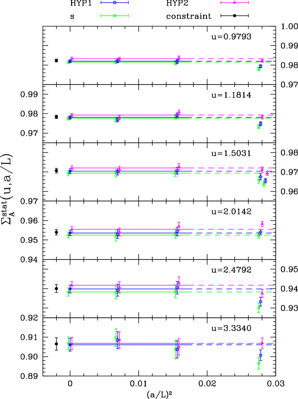
Figure 2: The lattice step scaling function $\Sigma_{\rm A}^{\rm stat}(u,a/L)$ and its continuum limit extrapolations to a constant omitting the $L/a=6$ data, separately for the three different static discretizations $S^{\text{s}}_{\mathrm{\,h}}$, $S^{\text{HYP1}}_{\mathrm{\,h}}$ and $S^{\text{HYP2}}_{\mathrm{\,h}}$ (colored lines). The black points (slightly shifted to the left of $a=0$) refer to the corresponding constrained $\chi^{2}$–minimization of the data from all three actions and give our final results for $\sigma_{\rm A}^{\rm stat}(u)$ in table 1. For the third smallest coupling, the two sets of points at $L/a=6$ refer to one-loop and two-loop values for the boundary improvement coefficient $c_{\rm t}$ [39, 40].

$u$		$\sigma_{\rm A}^{\rm stat}(u)$
$0.9793$		$0.9823(7)(2)$
$1.1814$		$0.9784(8)(11)$
$1.5031$		$0.9707(12)(3)$
$2.0142$		$0.9540(14)(9)$
$2.4792$		$0.9400(20)(4)$
$3.3340$		$0.9066(33)(25)$

Table 1: Results for the continuum step scaling function $\sigma_{\rm A}^{\rm stat}(u)$ from constrained fits to a constant, excluding the $L/a=6$ data. The first error is statistical, while the second one is the difference between the fit and the $L/a=8$ result and is accounted for as a systematic error.

With eq. (21) of section 2 it was already anticipated that the running of a renormalized matrix element of the static axial current in the SF scheme with $N_{\rm f}=2$ massless quark flavours can be extracted from the step scaling function $\sigma_{\rm A}^{\rm stat}(u)$, which is defined as the continuum limit of the lattice step scaling function $\Sigma_{\rm A}^{\rm stat}(u,a/L)$, i.e.

$$\sigma_{\rm A}^{\rm stat}(u)=\lim\limits_{a\to 0}\Sigma_{\rm A}^{\rm stat}(u,a/L)\;,\quad\Sigma_{\rm A}^{\rm stat}(u,a/L)=\left.{{Z_{\rm A}^{\rm stat}(g_{0},2L/a)}\over{Z_{\rm A}^{\rm stat}(g_{0},L/a)}}\,\right|_{\,\bar{g}^{2}(L)=u\,,\,m_{0}=m_{\rm c}}\;.$$ (23)

The condition $m_{0}=m_{\rm c}$, eq. (20), refers to lattice size $L/a$ and amounts to set the hopping parameter in the simulations to its critical value, $\kappa=\kappa_{\rm c}$. Enforcing $\bar{g}^{2}(L)$ to take some prescribed value $u$ fixes the bare coupling value $g_{0}^{2}=6/\beta$ to be used for given $L/a$. In this way, $\Sigma_{\rm A}^{\rm stat}$ becomes a function of the renormalized coupling $u$ up to cutoff effects and approaches its continuum limit as $a/L\rightarrow 0$ for fixed $u$.

We computed $Z_{\rm A}^{\rm stat}(u,a/L)$ at six values of $u$, where the corresponding box sizes cover a range of the order $L=0.01\,{\rm fm}\,\ldots\,1\,{\rm fm}$ (or $\mu$ in $20\,{\rm GeV}\,\ldots\,0.2\,{\rm GeV}$). At each $u$, three lattice resolutions — $L/a=6,8,12$ — were simulated, and the numerical results for $Z_{\rm A}^{\rm stat}$ and $\Sigma_{\rm A}^{\rm stat}$ stemming from the three static discretization s, HYP1 and HYP2 are collected in tables 5 and 6 in appendix B. Statistical errors were estimated by a jackknife analysis and cross-checked with the method of ref. [41].

Given the available data sets belonging to the static actions $i\in\{\text{s},\text{HYP1},\text{HYP2}\}$ as well as the fact that we work in (modulo $c_{\rm A}^{\rm stat}$, see appendix A) non-perturbatively ${\rm O}(a)$ improved QCD, there are basically two different ways to extrapolate the lattice step scaling function to the continuum. Either one can perform separate fits

$$\Sigma^{\text{stat}}_{\text{A,}i}(u,a/L)=\sigma^{\text{stat}}_{\text{A,}i}(u)+\rho_{i}(u)\times(a/L)^{2}$$ (24)

or, assuming universality of the continuum limit, a simultaneous extrapolation under the constraint of a common fit parameter $\sigma_{\rm A}^{\rm stat}$ in

$$\Sigma^{\text{stat}}_{\text{A,}i}(u,a/L)=\sigma_{\rm A}^{\rm stat}(u)+\rho^{\prime}_{i}(u)\times(a/L)^{2}\;.$$ (25)

Fit results from two examples of fits of the first kind are deferred to tables 7 and 8 in appendix B. These fits employ the ansatz (24), including the data at all available lattice resolutions in one case, whereas in the other case the coarsest data, $L/a=6$, are discarded and the fit ansatz is just a constant ($\rho\equiv 0$). The nice consistency of the two sets of results provides already clear evidence for the very weak overall lattice spacing dependence of the step scaling functions $\Sigma^{\text{stat}}_{\text{A,}i}(u,a/L)$, particularly beyond $L/a=6$, which can also be inferred from tables 5 and 6 by direct inspection of the raw data.

Our final extrapolation to the continuum is based on our experiences gained from the quantitative investigations of the running of the QCD coupling and quark masses in the SF scheme [19, 20], where the cutoff effects of the corresponding step scaling functions were found to be very small as well. The continuum limits were thus obtained according to eq. (25) by fitting the two values of $\Sigma^{\text{stat}}_{\text{A,}i}$ on the finer lattices ($L/a=8,12$) simultaneously for $i\in\{\text{s},\text{HYP1},\text{HYP2}\}$ to a common constant $\sigma_{\rm A}^{\rm stat}$ ($\rho^{\prime}\equiv 0$), separately for each coupling $u$. We then added linearly the difference between the fit and the $L/a=8$ result as a systematic error. These constrained constant fits are displayed in figure 2, and the resulting pairs of $u$ and continuum values $\sigma_{\rm A}^{\rm stat}(u)$ are summarized in table 1. By explicitly trying various different extrapolations along the ansätze (24) and (25) (while not only quadratic but also linear in $a$) we verified with confidence that, within the achievable statistical accuracy, our data do not show any significant dependence on the lattice spacing and that the continuum limit is well under control.

3.2 Non-perturbative scale evolution

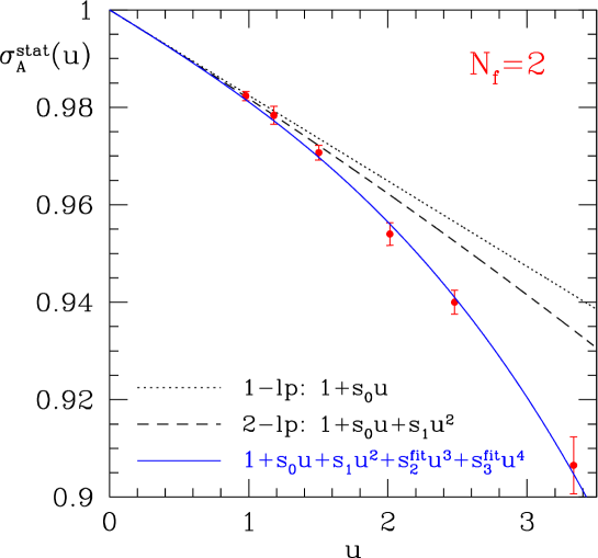
Figure 3: Continuum step scaling function $\sigma_{\rm A}^{\rm stat}(u)$ and its polynomial fit.

For the next steps of the analysis it is most convenient to represent the continuum step scaling function $\sigma_{\rm A}^{\rm stat}$ as a smooth function of $u$. To this end, we start from eq. (9) to write down the expression that relates $\sigma_{\rm A}^{\rm stat}(u)$ to the anomalous dimension $\gamma$ and the $\beta$–function, namely

$$\sigma_{\rm A}^{\rm stat}(u)=\exp\left\{-\int_{\sqrt{u}}^{\sqrt{\sigma(u)}}{\rm d}g\,\frac{\gamma(g)}{\beta(g)}\right\}\;,$$ (26)

where $\sigma(u)$ is the step scaling function of the coupling, determined by [19]

$$-2\ln(2)=\int_{u}^{\sigma(u)}{\rm d}x\,\frac{1}{\sqrt{x}\,\beta(\sqrt{x})}\;.$$ (27)

The first non-universal coefficients in the perturbative expansions of $\gamma$ and $\beta$ are given for the SF scheme by the two-loop result $\gamma_{1}$ as already quoted in (22) and the three-loop expression (cf. [19])

$$b_{2}=\frac{1}{(4\pi)^{3}}\,\Big{(}\,0.483-0.275N_{\rm f}+0.0361N_{\rm f}^{2}-0.00175N_{\rm f}^{3}\,\Big{)}\;.$$ (28)

These formulae imply that $\sigma_{\rm A}^{\rm stat}$ has a perturbative expansion of the form

$$\sigma_{\rm A}^{\rm stat}(u)=1+s_{0}u+s_{1}u^{2}+s_{2}u^{3}+\ldots$$ (29)

with, for instance, the two leading coefficients found to be

$$s_{0} = \ln(2)\gamma_{0}\;,$$ (30)

$$s_{1} = {\textstyle{\frac{1}{2}}}s_{0}^{2}+s_{0}\ln(2)b_{0}+\ln(2)\gamma_{1}\;.$$ (31)

Guided by eq. (29), we therefore represent the non-perturbative results for $\sigma_{\rm A}^{\rm stat}(u)$ in table 1 (with added statistical and systematic errors) by an interpolating fit to an ansatz polynomial in $u$, where $s_{0},s_{1}$ are restricted to their perturbative predictions and up to three additional free fit parameters are allowed for. All of these fits describe the data well, and we quote the two-parameter fit (the curve of which is shown in figure 3) as the final representation for the functional form of $\sigma_{\rm A}^{\rm stat}(u)$. The stability of the polynomial fits was further checked by fits with only $s_{0}$ (or even no coefficient at all) constrained to its perturbative value, which led to compatible results, including a fit to $(\sigma_{\rm A}^{\rm stat}(u)-1)/u=s_{0}+s_{1}u+\ldots$ to reproduce the perturbative prediction for $s_{0}$.

Moreover, figure 3 demonstrates — in contrast to previous calculations of the non-perturbative scale evolution within the SF scheme of other renormalized observables in quenched and two-flavor QCD [17, 18, 19, 20] — that the present case of the $N_{\rm f}=2$ static axial current provides another example for a significant deviation of the non–perturbative data from the perturbative behaviour, which even sets in already at moderate couplings $u$.

Now we use $\sigma_{\rm A}^{\rm stat}(u)$ given by the fit function in order to solve the following joint recursion to evolve the coupling and the renormalized matrix element $\Phi$ from a low-energy scale $1/L_{\rm max}$ implicitly defined by

$$u_{0}=\bar{g}^{2}(L_{\rm max})=4.61$$ (32)

to the higher energy scales $1/L_{k}$, $k=0,1,\ldots,8$ (with $L_{0}\equiv L_{\rm max}$):

$$u_{0}=4.61\;,\quad\sigma(u_{k+1})=u_{k} \quad\Rightarrow\quad u_{k}=\bar{g}^{2}(L_{k})\;,\quad L_{k}=2^{-k}L_{\rm max}\;,$$ (33)

$$v_{0}=1\;,\quad v_{k}=\left[\,\prod_{i=1}^{k}\sigma_{\rm A}^{\rm stat}(u_{i})\,\right]^{-1} \quad\Rightarrow\quad v_{k}=\frac{\Phi(1/L_{\rm max})}{\Phi(1/L_{k})}\;.$$ (34)

For this purpose, also the scale evolution of the coupling is parameterized by an interpolating polynomial of the form $\sigma(u)=u+\sigma_{0}u^{2}+\sigma_{1}u^{3}+\ldots\,$, for which the exact results of the corresponding fit (and its covariance matrix) were available from [20, 42]. Since the errors on the step scaling functions stem from different simulation runs and are hence uncorrelated, the errors on the fit parameters in the polynomials for $\sigma(u),\sigma_{\rm A}^{\rm stat}(u)$ and those on the recursion coefficients $u_{k},v_{k}$ calculated from them can be estimated and passed through the recursion straightforwardly by the standard error propagation rules.

3.3 The universal renormalization factor

			$\Phi_{\rm RGI}/\Phi(L_{\rm max}^{-1})$
$k$	$u$		2/3-loop		1/2-loop
0	4.610		0.853		0.851
1	3.032		0.863(3)		0.862
2	2.341		0.871(5)		0.870
3	1.918		0.875(6)		0.874
4	1.628		0.878(6)		0.877
5	1.414		0.879(7)		0.878
6	1.251		0.880(7)		0.879
7	1.121		0.880(7)		0.879
8	1.017		0.880(7)		0.880

Table 2: Evaluation of eq. (3.3), exploiting the perturbative knowledge of the $\gamma$– and $\beta$–functions in the SF scheme.

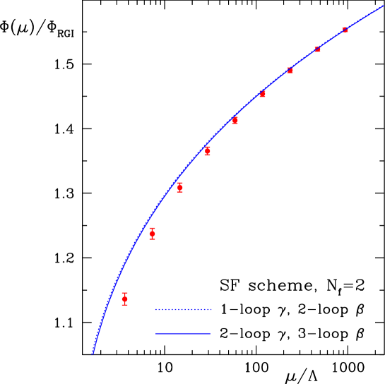
Figure 4: Numerically computed values of the running matrix element of the static axial current in the SF scheme compared to perturbation theory. The dotted and solid lines are obtained from eq. (9) using the 1/2– and 2/3–loop expressions for the $\gamma$– and $\beta$–functions, respectively, as well as $\ln(\Lambda L_{\rm max})=-1.298(58)$ from ref. [19].

Finally, by virtue of eqs. (9) and (34), we proceed to relate the renormalized matrix element $\Phi(\mu)=Z_{\rm A}^{\rm stat}(L)\Phi_{\rm bare}(g_{0})$, $\mu=1/L$, at $L=L_{\rm max}$ to the RGI one as

$$\frac{\Phi_{\rm RGI}}{\Phi(1/L_{\rm max})} = v_{k}^{-1}\,\frac{\Phi_{\rm RGI}}{\Phi(1/L_{k})}$$

$$= {Z_{\rm A}^{\rm stat}(2^{-k}L_{\rm max})\over Z_{\rm A}^{\rm stat}(L_{\rm max})}\,\left[\,2b_{0}\bar{g}^{2}(\mu)\,\right]^{-\gamma_{0}/(2b_{0})}\exp\left\{-\int_{0}^{\bar{g}(\mu)}{\rm d}g\left[\,{\gamma(g)\over\beta(g)}-{\gamma_{0}\over b_{0}g}\,\right]\right\}$$

with $\mu=2^{k}/L_{\rm max}$ and the ratios of $Z$–factors, $v_{k}$, to be taken from the non-perturbative solution of the recursion (34) discussed in the foregoing subsection. After numerical integration of the second factor, $\Phi_{\rm RGI}/\Phi(1/L_{k})$, with $\bar{g}^{2}=u_{k}$ by employing the perturbative expressions for the $\gamma$– and $\beta$–functions at two- and three-loop accuracy, respectively, we arrive at the series of numbers listed in table 2. For $k\geq 3$ they show a remarkable stability in the coupling $u_{k}$ such that we select $k=6$ — yielding

$$\frac{Z_{\rm A}^{\rm stat}(L_{\rm max})}{Z_{\rm A}^{\rm stat}(L)}=0.762(5)\quad\mbox{at}\quad L=2^{-6}L_{\rm max}$$ (36)

and the coupling value ($u_{6}$) entering the second factor in eq. (3.3) to lie safely in the perturbative regime — in order to obtain our central result

$$\frac{\Phi_{\rm RGI}}{\Phi(\mu)}=0.880(7)\quad\mbox{or}\quad\frac{\Phi(\mu)}{\Phi_{\rm RGI}}=1.137(9)\quad\mbox{at}\quad\mu=1/L_{\rm max}$$ (37)

in the SF scheme. Hence, through this analysis we have succeeded in connecting the low- and high-energy scales $L=L_{\rm max}$ and $L=2^{-6}L_{\rm max}$ non-perturbatively as intended.

Note that, since the continuum limit has been taken, any regularization dependence has been removed from the result (37) so that ideally the error on $\Phi(\mu)/\Phi_{\rm RGI}$ of about 0.8% should only be included in estimates on matrix elements in the continuum limit.

In figure 4 we compare the numerically computed running with the corresponding curves in perturbation theory. For the argument $\mu/\Lambda=1/(L_{k}\Lambda)$, $k=0,1,\ldots,8$, we plot the points $\Phi(1/L_{k})/\Phi_{\rm RGI}$ calculated from (3.3) using the universal result (37). Here, the physical scale $\Lambda$ is implicitly determined by $\ln(\Lambda L_{\rm max})=-1.298(58)$ resulting from the recursion (33) [19, 20], and the errors of the points in figure 4 come from the coefficients $v_{k}$. As expected from the behaviour of $\sigma_{\rm A}^{\rm stat}(u)$ in figure 3, this comparison between the non-perturbative and perturbative running again reveals that good agreement with the perturbative approximation is only observed at high scales, while the difference grows up to 5% towards smaller energies of the order $\mu\approx 4\Lambda$.

4 $Z_{\rm A}^{\rm stat}$ at the low-energy matching scale

$\beta$	$\kappa$	$L/a$	$\bar{g}^{2}(L)$		$Z^{\text{stat}}_{\text{A,s}}$	$Z^{\text{stat}}_{\text{A,HYP1}}$	$Z^{\text{stat}}_{\text{A,HYP2}}$	$c_{\rm A}^{\rm stat}$
5.20	0.13600	4	3.65(3)		0.84621(63)	0.84550(53)	0.88820(58)	1-lp
					0.84846(63)	0.85760(54)	0.95061(65)	0
		6	4.61(4)		0.79204(58)	0.79631(52)	0.84456(52)	1-lp
					0.79409(58)	0.80730(52)	0.90004(55)	0
5.29	0.13641	4	3.394(17)		0.85323(60)	0.85218(50)	0.89202(55)	1-lp
					0.85541(60)	0.86385(51)	0.95227(61)	0
		6	4.297(37)		0.79954(69)	0.80384(60)	0.85006(59)	1-lp
					0.80152(69)	0.81444(61)	0.90358(62)	0
		8	5.65(9)		0.75464(71)	0.76110(65)	0.80934(65)	1-lp
					0.75653(71)	0.77124(65)	0.86058(67)	0
5.40	0.13669	4	3.188(24)		0.86090(63)	0.85965(53)	0.90020(56)	1-lp
					0.86302(63)	0.87103(53)	0.95911(62)	0
		6	3.864(34)		0.81111(68)	0.81448(60)	0.85700(59)	1-lp
					0.81300(68)	0.82458(60)	0.90774(63)	0
		8	4.747(63)		0.77310(64)	0.77816(59)	0.82316(57)	1-lp
					0.77491(65)	0.78785(59)	0.87185(60)	0

Table 3: Results for $Z_{\rm A}^{\rm stat}$ with $c_{\rm t}$ set to its 2–loop value, both for $c_{\rm A}^{\rm stat}={\rm 1-loop}$ and $c_{\rm A}^{\rm stat}=0$. The values of $\bar{g}^{2}$ are from [19]. The hopping parameters $\kappa$ used in the simulations are taken to be the critical ones ($\kappa_{c}$) of [43].

$S_{\rm h}$		$\beta$		$Z_{\rm A}^{\rm stat}$		$Z_{\rm RGI}$		$c_{\rm A}^{\rm stat}$
s		5.20		0.7920(6)		0.6970(6)(56)		1-lp
				0.7941(6)		0.6988(6)(56)		0
		5.29		0.7873(28)		0.6928(28)(55)		1-lp
				0.7892(28)		0.6945(28)(56)		0
		5.40		0.7784(28)		0.6850(28)(55)		1-lp
				0.7802(28)		0.6866(28)(55)		0
HYP1		5.20		0.7962(5)		0.7007(5)(56)		1-lp
				0.8073(5)		0.7104(5)(57)		0
		5.29		0.7922(27)		0.6971(27)(56)		1-lp
				0.8026(27)		0.7063(27)(57)		0
		5.40		0.7832(26)		0.6892(26)(55)		1-lp
				0.7930(27)		0.6978(27)(56)		0
HYP2		5.20		0.8446(5)		0.7432(5)(59)		1-lp
				0.9000(5)		0.7920(5)(63)		0
		5.29		0.8390(25)		0.7383(25)(59)		1-lp
				0.8919(26)		0.7849(26)(63)		0
		5.40		0.8279(24)		0.7286(24)(58)		1-lp
				0.8769(26)		0.7717(26)(62)		0

Table 4: Results for $Z_{\rm A}^{\rm stat}$ and $Z_{\rm RGI}$ for three bare gauge coupling values corresponding to our low-energy matching point at $\bar{g}^{2}=4.61$ in the SF scheme, distinguishing the three static discretizations used.

Connecting a bare matrix element of the static-light axial current to the RGI one according to eq. (3) amounts to multiply the bare lattice operator with the total renormalization factor

$$Z_{\rm RGI}(g_{0})\equiv\left.\frac{\Phi_{\rm RGI}}{\Phi(\mu)}\,\right|_{\,\mu=1/L_{\rm max}}\,\times\,\left.Z_{\rm A}^{\rm stat}(g_{0},L/a)\,\right|_{\,L=L_{\rm max}}\;,$$ (38)

which involves — in addition to the universal ratio $\Phi_{\rm RGI}/\Phi(\mu)$, eq. (37) — the value of the renormalization factor $Z_{\rm A}^{\rm stat}(g_{0},L/a)$ at the finite, low-energy renormalization scale $L_{\rm max}$ implicitly fixed by the condition $\bar{g}^{2}(L_{\rm max})=4.61$ in the intermediate SF scheme.

Following the steps of the analogous computation in the case of the running quark mass in QCD [20], we now derive the second factor in eq. (38) for a few values of the lattice spacing or the bare coupling, respectively. As pointed out before, this contribution is non-universal, and in the form given it will be valid only for our static-light actions, consisting of non-perturbatively improved Wilson fermions with plaquette gauge action and $c_{\rm sw}$ as specified in [44] characterizing the light quark sector and the three discretizations s, HYP1 and HYP2 employed for the static quark flavour. For $c_{\rm A}^{\rm stat}$ we insert the one-loop values recently determined for these static actions in [38] and reproduced in appendix A. It thus remains to compute $Z_{\rm A}^{\rm stat}(g_{0},L_{\rm max}/a)$ for the values $\beta=5.2,5.29,5.4$, which lie well within the range of bare couplings commonly used in simulations of two-flavour QCD in physically large volumes. The associated simulation parameters and results are summarized in table 3. In order to allow for studying the influence of $c_{\rm A}^{\rm stat}$ on future continuum extrapolations of renormalized matrix elements, we also provide estimates for $Z_{\rm A}^{\rm stat}(g_{0},L/a)$ with $c_{\rm A}^{\rm stat}$ being set to zero.

While one of the simulations at the largest bare coupling is exactly at the target value for $\bar{g}^{2}$, the two other series of simulations require a slight interpolation. This has been done adopting a fit ansatz motivated by eq. (9),

$$\ln\left(Z_{\rm A}^{\rm stat}\right)=c_{1}+c_{2}\ln(\bar{g}^{2})\;,$$ (39)

to interpolate $Z_{\rm A}^{\rm stat}$ between those two values of $\bar{g}^{2}$ straddling the target value $4.61$, whereby the fit takes into account the (independent) errors of both $Z_{\rm A}^{\rm stat}$ and $\bar{g}^{2}$. We then augmented the fit error by the difference between the fit result via eq. (39) and the result from a simple two-point linear interpolation in $\bar{g}^{2}$. The values of the coefficient $c_{2}$ in the fit (39) are found to deviate not more than by about $0.03$ (with errors on the 7% level) from $\gamma_{0}/(2b_{0})=-6/29\approx-0.2069$.

The resulting numbers for $Z_{\rm A}^{\rm stat}(g_{0},L_{\rm max}/a)$ and finally for the total renormalization factor $Z_{\rm RGI}(g_{0})$, cf. eq. (38), are collected in table 4. The first error on $Z_{\rm RGI}$ stems from the error of $Z_{\rm A}^{\rm stat}$, whereas the second one embodies the 0.8% uncertainty in the universal factor $\Phi_{\rm RGI}/\Phi$ and, provided that the renormalized matrix element of the static current is available at several lattice spacings, should not be added in quadrature to the error on the latter before the continuum limit has eventually been taken. For later use, a representation of the numerical results of table 4 by interpolating polynomials can be found in table 9 in appendix B. Comparing the cases $c_{\rm A}^{\rm stat}={\rm 1-loop}$ and $c_{\rm A}^{\rm stat}=0$, we observe that only for the static action HYP2 the change in the renormalization factors is about 6% and thereby non-negligible, which however can be attributed to the fact that for this action the one-loop coefficient of $c_{\rm A}^{\rm stat}$ is by one order of magnitude larger than for the static discretization HYP1 (cf. eq. (63)).

5 Matrix elements at finite values of the quark mass

It was already outlined in the introduction that in order to employ results from the static effective theory, one has to translate its RGI matrix elements to those in QCD at finite values of the heavy quark mass. For the special case of the matrix element of the axial current between the vacuum and the heavy-light pseudoscalar, this conversion to the so-called ‘matching scheme’ amounts to a multiplication with a function $C_{\rm PS}(M/\Lambda_{\overline{{\rm MS}}})$, viz.

$$F_{\rm PS}\sqrt{m_{\rm PS}}=C_{\rm PS}\left(M/\Lambda_{\overline{{\rm MS}}}\right)\Phi_{\rm RGI}=C_{\rm PS}\left(M/\Lambda_{\overline{{\rm MS}}}\right)Z_{\rm RGI}\langle\,{\rm PS}\,|\,A^{\rm stat}_{0}\,|\,0\,\rangle$$ (40)

up to ${\rm O}(1/M)$ corrections, where it is theoretically as well as practically advantageous to express $C_{\rm PS}$ in terms of a ratio of RGIs as [17, 45]

$$C_{\rm PS}\left(M/\Lambda_{\overline{{\rm MS}}}\right)=\left[\,2b_{0}\bar{g}_{{\rm\overline{MS\kern-0.35002pt}\kern 0.35002pt}}^{2}\,\right]^{\gamma_{0}/(2b_{0})}\exp\left\{\int_{0}^{\bar{g}_{{\rm\overline{MS\kern-0.25002pt}\kern 0.25002pt}}}{\rm d}g\left[\,{\gamma^{\rm match}(g)\over\beta(g)}-{\gamma_{0}\over b_{0}g}\,\right]\right\}\;;$$ (41)

$\gamma^{\rm match}$ denotes the anomalous dimension of the current in the matching scheme. As we will see in the next subsection, $C_{\rm PS}$ is very well under control in perturbation theory.

To exploit eq. (40) in order to determine the decay constant $F_{\rm PS}$, after having non-perturbatively solved the renormalization problem of the static axial current, is the main purpose of this section.

5.1 Perturbative evaluation of the conversion function

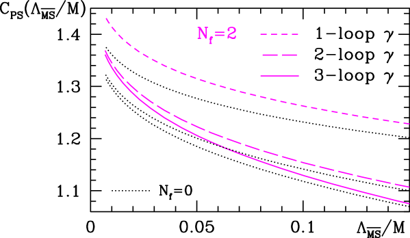
Figure 5: $N_{\rm f}=2$ conversion factor to the matching scheme, which translates the RGI matrix element of $A^{\rm stat}_{0}$ to the one at finite mass. A continuous parameterization using the anomalous dimension $\gamma$ to two- and three-loop accuracy, respectively, is given in eq. (46). The dotted curves show the corresponding conversion function for $N_{\rm f}=0$ [17, 45] for comparison.

The numerical evaluation of the perturbative approximation of the conversion function $C_{\rm PS}(M/\Lambda_{\rm\overline{MS}})$ has been explained in detail in appendix B of ref. [45]. This analysis is straightforwardly extended to the present case of two-flavour QCD, $N_{\rm f}=2$: Using the anomalous dimension in the matching scheme that involves (i) the anomalous dimension of the corresponding effective theory operator in the $\overline{\rm MS}$ scheme up to three-loop order [21, 46, 47, 48] and (ii) matching coefficients between the effective theory and physical QCD operator up to two loops [5, 36, 49] — together with the four-loop $\beta$–function [50] and quark mass anomalous dimension [51, 52] in the $\overline{\rm MS}$ scheme —, the numerically evaluated conversion function $C_{\rm PS}(M/\Lambda_{\rm\overline{MS}})$ is shown in figure 5.

As in the quenched case [17, 45] it is actually more convenient to represent $C_{\rm PS}$ as a continuous function in terms of the variable

$$x\equiv\frac{1}{\ln\left(M/\Lambda_{{\rm\overline{MS\kern-0.35002pt}\kern 0.35002pt}}\right)}$$ (42)

in a form that is motivated by eq. (9). This results in

$$N_{\rm f}=2:\quad C_{\rm PS}(x)=\left\{\begin{array}[]{ll}x^{\gamma_{0}/(2b_{0})}\left\{\,1-0.107\,x+0.093\,x^{2}\,\right\}&\;\;\mbox{2--loop $\gamma$}\\ \\ x^{\gamma_{0}/(2b_{0})}\left\{\,1-0.118\,x-0.010\,x^{2}+0.043\,x^{3}\,\right\}&\;\;\mbox{3--loop $\gamma$}\end{array}\right.\,,$$ (46)

with $b_{0}=(11-\frac{2}{3}N_{\rm f})/(4\pi)^{2}$ and $\gamma_{0}=-1/(4\pi^{2})$, whereby the prefactor encodes the leading asymptotics as $x\rightarrow 0$. For 3–loop $\gamma$, the precision of the parameterization (46) is at least 0.2% for $x\leq 0.6$, and one may attribute an error of at most 2% owing to the perturbative approximation underlying this determination of the conversion function.

For future purposes, we also quote the corresponding parameterization for the three-flavour theory:

$$N_{\rm f}=3:\quad C_{\rm PS}(x)=\left\{\begin{array}[]{ll}x^{\gamma_{0}/(2b_{0})}\left\{\,1-0.144\,x+0.130\,x^{2}\,\right\}&\;\;\mbox{2--loop $\gamma$}\\ \\ x^{\gamma_{0}/(2b_{0})}\left\{\,1-0.161\,x+0.062\,x^{2}+0.007\,x^{3}\,\right\}&\;\;\mbox{3--loop $\gamma$}\end{array}\right.\,.$$ (50)

5.2 Application: non-perturbative renormalization of $F_{{\rm B}_{\rm s}}^{\rm stat}$

For an immediate use of the results obtained, we present a first non-perturbative computation of the decay constant $F_{\rm B_{\rm s}}$ in the static limit, based on data for the bare matrix element of $A^{\rm stat}_{0}$ in large volume and for the static action $S^{\text{HYP2}}_{\mathrm{\,h}}$. To this end we have used one of the sets of unquenched (two degenerate flavours) configurations produced by the ALPHA Collaboration for setting the scale for the $N_{\rm f}=2$ $\Lambda$–parameter and RGI quark mass [19, 20] by simulations in physically large volumes [22, 53]. The bare parameters are given by $\beta=5.3$, $\kappa=0.1355$, $V=24^{3}\times 32$, and the RGI light quark mass [20] turns out to be $171(4)\,{\rm MeV}$. For the conversion to MeV we have used $a=0.078(1)\,{\rm fm}$ at $\beta=5.3$ as given in ref. [54]. The value of the quark mass is at the upper end of the result for $M_{\rm s}$ in [20] (i.e. $M_{\rm s}=138(31)\,{\rm MeV}$). Anyway, the dependence of $F_{\rm B_{\rm s}}$ on the exact value of $M_{\rm s}$ is expected to be quite mild, as the JLQCD Collaboration, for instance, has reported ${F_{\rm B_{\rm s}}}/{F_{\rm B_{\rm u}}}=1.13(3)(^{+13}_{-2})$ in ref. [55]. According to that we would have to correct our result on $F_{\rm B_{\rm s}}$ by decreasing it by about $3\%$. Such a correction is however below the $5\%$ statistical error we are able to achieve at this lattice resolution.

The computational details closely follow what has been done in the quenched case discussed in refs. [13, 15]. To suppress excited B-meson state contributions to the correlation functions, we introduce wave functions $\omega({\bf x})$ at the boundaries of the SF such that the correlators $f_{\rm A}^{\rm stat}$ and $f_{1}^{\rm stat}$ (cf. eqs. (13) – (15) in section 2) take the form

$$f_{\rm A}^{\rm stat}(x_{0},\omega_{i})=-{{1}\over{2}}\left\langle(A_{\rm I}^{\rm stat})_{0}(x)\,{\cal{O}}(\omega_{i})\right\rangle\;,\quad f_{1}^{\rm stat}(\omega_{i},\omega_{j})=-{{1}\over{2}}\left\langle{\cal{O}}^{\prime}(\omega_{i})\,{\cal{O}}(\omega_{j})\right\rangle\;,$$ (51)

with

$${\cal O}(\omega)={{a^{6}}\over{L^{3}}}\sum_{\bf y,z}\overline{\zeta}_{\rm h}({\bf y})\gamma_{5}\,\omega({\bf y}-{\bf z})\,\zeta_{\rm l}({\bf z})\;,\quad{\cal O}^{\prime}(\omega)={{a^{6}}\over{L^{3}}}\sum_{\bf y,z}\overline{\zeta}_{\rm l}^{\prime}({\bf y})\gamma_{5}\,\omega({\bf y}-{\bf z})\,\zeta_{\rm h}^{\prime}({\bf z})\;,$$ (52)

and the improved version $(A_{\rm I}^{\rm stat})_{0}$ of the static-light axial current defined as

$$(A_{\rm I}^{\rm stat})_{0}(x)=A^{\rm stat}_{0}(x)+a\,c_{\rm A}^{\rm stat}\delta A_{0}^{\rm stat}(x)\;.$$ (53)

We restrict ourselves to a choice of four spatially periodic wave functions

$$\omega_{i}({\bf x}) = \frac{1}{N_{i}}\sum_{\bf n\,\in\,\mathbb{Z}^{3}}\overline{\omega}_{i}\left(|{\bf x-n}L|\right)\;,\quad i=1,\dots,4\;,$$

$$\overline{\omega}_{1}(r) = a^{\,-3/2}\,{\rm e}^{\,-r/a}\;,\qquad\overline{\omega}_{2}(r)=a^{\,-3/2}\,{\rm e}^{\,-r/2a}\;,$$

$$\overline{\omega}_{3}(r) = a^{\,-5/2}\,r\,{\rm e}^{\,-r/2a}\;,\quad\overline{\omega}_{4}(r)=a^{\,-3/2}\,{\rm e}^{\,-r/4a}\;,$$ (54)

with the coefficients $N_{i}$ normalizing them such that $a^{3}\sum_{\bf x}\omega_{i}^{2}({\bf x})=1$ holds. Numerically, we have approximated the wave functions using the lowest six Fourier components in each spatial (positive and negative) direction. That reduces the computational cost for the convolutions required to calculate $f_{1}^{\rm stat}$.

The decay constant is then extracted from the expression for the local RGI matrix element of the static axial current,

$$\Phi_{\rm RGI}(x_{0},\omega_{i})=-Z_{\rm RGI}\left(1+b_{\rm A}^{\rm stat}am_{\rm q}\right)2L^{3/2}\,{{f_{\rm A}^{\rm stat}(x_{0},\omega_{i})}\over{\sqrt{f_{1}^{\rm stat}(\omega_{i},\omega_{i})}}}\,{\rm e}^{\,(x_{0}-T/2)E_{\rm eff}(x_{0},\omega_{i})}\;,$$ (55)

where for $b_{\rm A}^{\rm stat}$ the one-loop formula for the static discretization $S^{\text{HYP2}}_{\mathrm{\,h}}$ from ref. [38] enters. The effective energy $E_{\rm eff}$ reads

$$E_{\rm eff}(x_{0},\omega_{i})=\frac{1}{2a}\ln\left[\,\frac{f_{\rm A}^{\rm stat}(x_{0}-a,\omega_{i})}{f_{\rm A}^{\rm stat}(x_{0}+a,\omega_{i})}\,\right]$$ (56)

and is shown in figure 6 for the wave function $\omega_{2}$. This choice is motivated by the fact that $E_{\rm eff}(x_{0},\omega_{2})$ approaches its plateau value earlier than it is the case for the other wave functions (which anyway yield consistent values for $x_{0}\gtrsim 1.4\,{\rm fm}$). The corresponding bare decay constant $\Phi_{\rm bare}$, i.e. the quantity in eq. (55) with $Z_{\rm RGI}$ set to one and $b_{\rm A}$ set to zero, is displayed in figure 7. Proper linear combinations built from correlators affiliated to the other wave functions lead to fully compatible graphs.

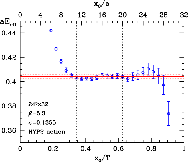
Figure 6: Effective energy for the wave function $\omega_{2}$. The plateau region is limited by the dotted vertical lines while the horizontal band is the resulting plateau average.

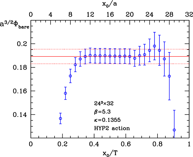
Figure 7: Effective bare decay constant for the same parameters as in figure 6. Note that, contrary to the effective energy, in this case the horizontal band does not correspond to a plateau average but to the value for $\Phi_{\rm bare}$ as obtained from the two-state fits of $f_{\rm A}^{\rm stat}(x_{0},\omega_{2})$ (see text).

Given the clear plateau in the effective mass, we simply fit it to a constant in the region $11\leq x_{0}/a\leq 20$ and obtain the result $aE_{\rm stat}=0.4042(15)$. Alternatively, we perform a two-state fit of $aE_{\rm eff}(x_{0},\omega_{2})$ to the function $aE_{\rm stat}+b_{1}\,{\rm e}^{\,-\Delta^{\rm stat}x_{0}}$ in the range $t_{\rm min}\leq x_{0}/a\leq 20$, with $t_{\min}\geq 4$. The results for $E_{\rm stat}$ from the two fits are in complete agreement. In addition, in the second case we get numbers for the energy gap $a\Delta^{\rm stat}$, which range between $0.5$ and $0.7$ depending on the choice for $t_{\rm min}$. At the same lattice spacing, the binding energy $aE_{\rm stat}$ from the static HYP-actions in the quenched theory turned out to be approximately 10% smaller [12, 15]. This is the relative effect one could have guessed by using the one-loop expression for the static quark self-energy, considering the shift in $\beta$ between the quenched and the $N_{\rm f}=2$ theory (i.e. $\beta=6.1$ versus $\beta=5.3$, respectively, for $a\approx 0.08\,{\rm fm}$). Thus, the noise-to-signal ratio of the correlation function, which is governed by $aE_{\rm stat}$ and the mass of the lightest pseudoscalar [58], is comparable in both cases.

For $\Phi_{\rm bare}$, rather than directly fitting it to a constant within the plateau region, we first fit the correlation function $f_{\rm A}^{\rm stat}(x_{0},\omega_{2})$ to the two-state ansatz $b_{2}\,{\rm e}^{\,-E_{\rm stat}x_{0}}+b_{3}\,{\rm e}^{\,-(E_{\rm stat}+\Delta^{\rm stat})x_{0}}$ in order to extract in a second step $\Phi_{\rm bare}$ through the ratio of the coefficient $b_{2}$ and the square root of $f_{1}^{\rm stat}(\omega_{2},\omega_{2})$, as suggested by formula (55). In this way rather precise data could be used in the fit, because the main contribution to the statistical error of the effective decay constant comes from $f_{1}^{\rm stat}$. Moreover, we verified numerically that possible excited state contaminations in $f_{1}^{\rm stat}(\omega_{2},\omega_{2})$ are strongly suppressed and hence can be safely neglected. For varying fit intervals $t_{\rm min}\leq x_{0}/a\leq 20$ with $4\leq t_{\min}\leq 8$, this procedure yields stable numbers that are well covered by $\Phi_{\rm bare}=0.1892(62)$. More details will be provided in a forthcoming publication [15] extending ref. [13] which, as stated above, we follow quite closely here.

Combining the result on $\Phi_{\rm bare}$ with eq. (37), $Z_{\rm A}^{\rm stat}(g_{0},L_{\rm max}/a)|_{\beta=5.3}=0.8382(25)$ (obtained from the interpolation quoted at the end of appendix B) and $am_{\rm q}=0.0260(3)$, we get according to eq. (55):

$$a^{3/2}\Phi_{\rm RGI}=0.143(5)\;.$$ (57)

Finally, inserting the proper value of the conversion function $C_{\rm PS}(M_{\rm b}/\Lambda_{\rm\overline{MS}})=1.24(3)$ (after evaluation of the three-loop expression in (46) from the previous subsection) into eq. (40), we arrive at $F_{{\rm B}_{\rm s}}^{\rm stat}=306(14)\,{\rm MeV}$, where $m_{{\rm B}_{\rm s}}=5368(2)\,{\rm MeV}$ from ref. [59] has been employed. The quoted error accounts for the statistical uncertainty and the errors of the (universal and discretization dependent parts of the) renormalization factor as well as for the errors of the lattice spacing and of $C_{\rm PS}$. It should be recalled, though, that the light quark mass value of the data set analyzed and discussed in this section is still slightly above the physical strange quark mass. If the aforementioned decrease by $3\%$ to better meet the strange quark mass scale is incorporated, our estimate for the ${\rm B}_{\rm s}$-meson decay constant in static approximation at a finite lattice spacing of $a\approx 0.08\,{\rm fm}$ reads

$$F_{{\rm B}_{\rm s}}^{\rm stat}=297(14)\,{\rm MeV}\;.$$ (58)

This is broadly compatible with the $N_{\rm f}=2$ result $F_{{\rm B}_{\rm s}}^{\rm stat}=256(45)\,{\rm MeV}$ in the static approximation reported in ref. [56] by the UKQCD Collaboration, which however was determined at a coarser lattice spacing of $a\approx 0.1\,{\rm fm}$ ($\beta=5.2$) and which rests upon the Eichten-Hill static quark action and only perturbative renormalization.

We can get an idea about discretization effects from the quenched ($N_{\rm f}=0$) computation [15] of the very same quantity, again using O($a$) improved Wilson fermions and plaquette gauge action but the HYP1 action for the static quark. There, $F_{{\rm B}_{\rm s}}^{\rm stat}$ in the continuum turned out to be $233(18)\,{\rm MeV}$, and in that case the value of $F_{{\rm B}_{\rm s}}^{\rm stat}$ becomes about $10\%$ larger at $a\approx 0.08\,{\rm fm}$ than the continuum limit [15]. Therefore, our result indicates an increase in the two-flavour theory either for the value of $F_{\rm B_{\rm s}}$, as already observed in ref. [3], or for the ${\rm O}(1/m_{\rm b})$–corrections to the decay constant.

6 Conclusions

We have presented a solution of the scale dependent renormalization problem of the static axial current in two-flavour QCD by means of a fully non-perturbative computation of the renormalization group running of arbitrary renormalized matrix elements $\Phi$ of $A^{\rm stat}_{0}$ in the Schrödinger functional scheme. In particular, the renormalization factor $\Phi_{\rm RGI}/\Phi(\mu)$ relating the matrix element at a specified low-energy scale $\mu$ with the associated RG invariant in the continuum limit, eq. (37), is obtained with a good numerical precision, which is comparable with the corresponding study in the quenched approximation [17]. This is an important prerequisite for a controlled determination of $F_{\rm B}$ in the static limit of the two-flavour theory.

The use of the alternative discretization schemes of refs. [13, 38] for the static quark instead of the traditional Eichten-Hill action has not only led to a substantial reduction of the statistical errors of the static-light correlation functions involved in our computation, but also entails a convincing universality test of the continuum limit of the current’s lattice step scaling function (cf. figure 2). Similar to the case of the renormalized quark mass in $N_{\rm f}=2$ [20], we find this function to be nearly independent of the lattice spacing for $a/L<1/6$ and hence conclude that O($a$) improvement is very successful also at large values of the SF coupling. Contrary to the running of the quark mass, however, the scale evolution of the non-perturbative step scaling function of the renormalized static-light axial current, figure 3, exhibits a pronounced deviation from perturbation theory already at moderate couplings.

As a first application, we have combined our non-perturbative renormalization factors with a numerical result for the bare matrix element of $A^{\rm stat}_{0}$ extracted from a large-volume $N_{\rm f}=2$ simulation, in order to estimate the ${\rm B}_{\rm s}$-meson decay constant in the static limit for one value of the lattice spacing, $a\approx 0.08\,{\rm fm}$. In QCD with dynamical quarks, the static approximation may even be the starting point of the most viable approach to determine $F_{\rm B}$, especially if such a computation is supplemented with data on the heavy-light decay constant from the charm quark mass region (as already demonstrated in the quenched case [13, 15]) or with $1/M$–corrections. For a controlled inclusion of the latter, also the matching between the effective theory and QCD inherent in the conversion function $C_{\rm PS}$ (cf. eq. (40)) should then be performed non-perturbatively [8]. A general framework for this is provided by the non-perturbative formulation of HQET exposed in ref. [10]. Other approaches, such as the method of heavy quark mass extrapolations of finite-volume effects in QCD [60] and its conjunction with HQET [61], have been proven to be feasible in quenched QCD and yield consistent results there, but it may turn out to be difficult to extended them to the dynamical case.

With $F_{{\rm B}_{\rm s}}^{\rm stat}=297(14)\,{\rm MeV}$ at $a\approx 0.08\,{\rm fm}$ we find a value for the static decay constant that is significantly larger than the $N_{\rm f}=0$ estimate $F_{\rm B_{\rm s}}=194(6)\,{\rm MeV}$ quoted as the best quenched result in the recent review by Onogi [3]. This signals a visible effect of the dynamical fermions in the two-flavour theory — qualitatively in line with the outcome of other unquenched calculations [3] — which in the end could reflect in an increase of $F_{\rm B_{\rm s}}$ and/or its $1/M$–corrections to the static limit. Of course, these issues deserve further investigations and can only be settled if the two remaining sources of systematic errors are overcome, namely the yet slightly too large value of the sea quark mass and the lack of a continuum limit for $F_{{\rm B}_{\rm s}}^{\rm stat}$. Therefore, the reduction of the sea quark mass as well as a determination of the bare static-light decay constant for a smaller lattice resolution are part of an ongoing project [22]. Rather in the long term, also an active strange quark ($N_{\rm f}=2+1$) will have to be included.

Appendix A Lattice actions for the static quark sector

We use three discretizations of the action for static quarks, introduced in refs. [13, 38] to yield an exponential improvement of the signal-to-noise ratio in static-light correlation functions compared to the standard Eichten-Hill action [5],

$$S_{\rm h}[U,\overline{\psi}_{\rm h},\psi_{\rm h}]=a^{4}\sum_{x}\overline{\psi}_{\rm h}(x)D_{0}\psi_{\rm h}(x)\;,$$ (59)

$D_{0}$ being the time component of the backward lattice derivative acting on the heavy quark field $\psi_{\rm h}(x)$. These new static quark actions rely on changes of the form $U(x,0)\rightarrow W(x,0)$ of the parallel transporters $U(x,\mu)$ in the covariant derivative,

$$D_{0}\psi_{\rm h}(x)=\frac{1}{a}\left[\,\psi_{\rm h}(x)-W^{\dagger}(x-a\hat{0},0)\psi_{\rm h}(x-a\hat{0})\,\right]\;,$$ (60)

where now $W(x,0)$ is a function of the gauge fields in the immediate neighborhood of $x$ and $x+a\hat{0}$. In the numerical simulations and the data analysis underlying the present work we have considered, among the possible choices for $W(x,0)$, the regularized actions

$$W(x,0)=V(x,0)\left[\,\frac{g_{0}^{2}}{5}+\left({\textstyle{\frac{1}{3}}}\,{\rm Tr}\,V^{\dagger}(x,0)V(x,0)\right)^{1/2}\,\right]^{-1} \quad\Rightarrow\quad S^{\text{s}}_{\mathrm{\,h}}\;,$$ (61)

$$W(x,0)=V_{\rm HYP}(x,0) \quad\Rightarrow\quad S^{\text{HYP}}_{\mathrm{\,h}}\;,$$ (62)

where $V(x,0)$ is the average of the six staples around the link $U(x,0)$ and $V_{\rm HYP}(x,0)$ the HYP-link, the latter being a function of the gauge links located within a hypercube [62]. The ‘HYP-smearing’ involved in the construction of the HYP-link requires to further specify a triplet of coefficients, the two choices $(\alpha_{1},\alpha_{2},\alpha_{3})=(0.75,0.6,0.3)$ and $(\alpha_{1},\alpha_{2},\alpha_{3})=(1.0,1.0,0.5)$ of which were motivated in [62] and [38], respectively, and define the associated static actions $S^{\text{HYP1}}_{\mathrm{\,h}}$ and $S^{\text{HYP2}}_{\mathrm{\,h}}$. The discretization $S^{\text{s}}_{\mathrm{\,h}}$ is inspired by the SU(3) one-link integral, for which $W(x,0)$ in the form of eq. (61) is an approximation. For more details the reader may consult ref. [38]. In the text, we will also frequently distinguish these three static actions by just referring to them as ‘s’, HYP1 and HYP2.

While the largest improvement in statistical precision is actually achieved for the action HYP2, it is observed [13, 38] that generally with all the proposed discretizations at least an order of magnitude in the signal-to-noise ratios of B-meson correlation functions in the static approximation can be gained at time separations around $x_{0}\approx 1.5\,{\rm fm}$ w.r.t. the action (59) and that, in addition, the statistical errors grow only slowly as $x_{0}$ is increased. Even more importantly, quite the same small scaling violations in the ${\rm O}(a)$ improved theory are encountered with the new discretizations [38].

In that reference, also the (regularization dependent) improvement coefficient $c_{\rm A}^{\rm stat}$ multiplying the ${\rm O}(a)$ correction (16) to the static-light axial current has been numerically determined in one-loop order of perturbation theory, and we here reproduce the corresponding expansions for the three static quark discretizations at our disposal:

$$c_{\rm A}^{\rm stat}(g_{0})=c_{\rm A}^{\rm stat,(1)}\times g_{0}^{2}\quad\mbox{with}\quad c_{\rm A}^{\rm stat,(1)}=\left\{\begin{array}[]{lll}0.0072(4)&&\mbox{for $S^{\text{s}}_{\mathrm{\,h}}$}\\ 0.039(4)&&\mbox{for $S^{\text{HYP1}}_{\mathrm{\,h}}$}\\ 0.220(14)&&\mbox{for $S^{\text{HYP2}}_{\mathrm{\,h}}$}\end{array}\right.\;.$$ (63)

Appendix B Simulation results for $Z_{\rm A}^{\rm stat}$

In tables 5 and 6 we collect the bare parameters and results of our simulations to compute $Z_{\rm A}^{\rm stat}$. The pairs $(L/a,\beta)$ and the associated values of the critical hopping parameter, $\kappa=\kappa_{\rm c}$, were already known from the non-perturbative computation of the running of the Schrödinger functional coupling itself [19].

In order to extract the lattice step scaling function $\Sigma_{\rm A}^{\rm stat}$ according to eq. (23), simulations on lattices with linear extensions $L/a$ and $2L/a$ are required. At the three lowest couplings $\bar{g}^{2}(L)$, the runs have been performed using the one-loop value of the boundary ${\rm O}(a)$ improvement coefficient $c_{\rm t}$ in the gauge sector [39],

$$c_{\rm t}^{\rm 1-lp}(g_{0})=1-0.051\,g_{0}^{2}\;,$$ (64)

except for $\beta=7.542$ at $L/a=6$ and $\beta=7.7206$ at $L/a=8$. For these parameters as well as for the larger couplings the two-loop value of $c_{\rm t}$ [40],

$$c_{\rm t}^{\rm 2-lp}(g_{0})=1-0.051\,g_{0}^{2}-0.030\,g_{0}^{4}\;,$$ (65)

has been employed. At the third lowest coupling, $u\approx 1.5$, we checked at $L/a=6$ that there is no significant difference in $\Sigma_{\rm A}^{\rm stat}$ using the one- or two-loop value for $c_{\rm t}$. This is also illustrated by the additional data points included in figure 2. For decreasing $a/L$, the effect of the accuracy in $c_{\rm t}$ on the results is expected to become even smaller. The contribution to the error of $\Sigma_{\rm A}^{\rm stat}$ induced by the uncertainty in the coupling $u$ (which can be estimated with the aid of the one-loop result $\ln(2)\gamma_{0}$ for the derivative of $\sigma_{\rm A}^{\rm stat}$ with respect to $u$) is negligible compared to the statistical error of $\Sigma_{\rm A}^{\rm stat}$.

Tables 7 and 8 list the results of the alternative continuum limit extrapolations of the lattice step scaling function mentioned within the discussion in Section 3.1, which were performed as separate fits of the three data sets corresponding to the static actions s, HYP1 and HYP2.

Finally, we summarize in table 9 the coefficients $z_{i},f_{i}$ of the polynomial interpolations as functions of $5.2\leq\beta=6/g_{0}^{2}\leq 5.4$,

$$Z_{\rm A}^{\rm stat}(g_{0},L_{\rm max}/a)=\sum_{i=0}^{2}z_{i}\,(\beta-5.2)^{i}\;,\quad Z_{\rm RGI}(g_{0})=\sum_{i=0}^{2}f_{i}\,(\beta-5.2)^{i}\;,$$ (66)

of the numerical results on the renormalization factors $Z_{\rm A}^{\rm stat}(g_{0},L_{\rm max}/a)$ and $Z_{\rm RGI}(g_{0})$ tabulated in section 4. The statistical uncertainty to be taken into account when using these formulae varies between 0.1% ($\beta=5.2$) and about 0.3% ($\beta=5.4$). Only in the case of $Z_{\rm RGI}$, the additional 0.8% error of its regularization independent part (37) needs to be included.

				$S^{\text{s}}_{\mathrm{\,h}}$
$\bar{g}^{2}(L)$	$\beta$	$\kappa$	$L/a$	$Z_{\rm A}^{\rm stat}(L/a)$	$Z_{\rm A}^{\rm stat}(2L/a)$	$\Sigma_{\rm A}^{\rm stat}(u,a/L)$
0.9793	9.50000	0.131532	6	0.9396(5)	0.9190(7)	0.9782(8)
	9.73410	0.131305	8	0.9321(6)	0.9146(9)	0.9813(11)
	10.05755	0.131069	12	0.9253(4)	0.9083(7)	0.9816(9)
1.1814	8.50000	0.132509	6	0.9277(4)	0.9030(9)	0.9733(10)
	8.72230	0.132291	8	0.9195(7)	0.8997(10)	0.9785(13)
	8.99366	0.131975	12	0.9115(4)	0.8903(11)	0.9768(12)
1.5031	7.50000	0.133815	6	0.9095(6)	0.8783(14)	0.9658(17)
	8.02599	0.133063	12	0.8922(8)	0.8649(14)	0.9694(19)
1.5078	7.54200	0.133705	6	0.9110(6)	0.8780(9)	0.9638(12)
	7.72060	0.133497	8	0.9012(11)	0.8736(13)	0.9694(18)
2.0142	6.60850	0.135260	6	0.8843(9)	0.8422(11)	0.9525(15)
	6.82170	0.134891	8	0.8752(15)	0.8343(16)	0.9533(24)
	7.09300	0.134432	12	0.8636(11)	0.8219(17)	0.9518(23)
2.4792	6.13300	0.136110	6	0.8623(11)	0.8021(18)	0.9302(24)
	6.32290	0.135767	8	0.8506(16)	0.7984(25)	0.9386(34)
	6.63164	0.135227	12	0.8417(9)	0.7894(24)	0.9379(32)
3.3340	5.62150	0.136665	6	0.8310(13)	0.7450(22)	0.8965(29)
	5.80970	0.136608	8	0.8152(14)	0.7367(36)	0.9037(47)
	6.11816	0.136139	12	0.8061(14)	0.7333(35)	0.9097(46)

Table 5: Results for the step scaling function $\Sigma_{\rm A}^{\rm stat}$ with discretization $S^{\text{s}}_{\mathrm{\,h}}$.

				$S^{\text{HYP1}}_{\mathrm{\,h}}$			$S^{\text{HYP2}}_{\mathrm{\,h}}$
$\bar{g}^{2}(L)$	$\beta$	$\kappa$	$L/a$	$Z_{\rm A}^{\rm stat}(L/a)$	$Z_{\rm A}^{\rm stat}(2L/a)$	$\Sigma_{\rm A}^{\rm stat}(u,a/L)$	$Z_{\rm A}^{\rm stat}(L/a)$	$Z_{\rm A}^{\rm stat}(2L/a)$	$\Sigma_{\rm A}^{\rm stat}(u,a/L)$
0.9793	9.50000	0.131532	6	0.9360(5)	0.9167(6)	0.9794(8)	0.9503(5)	0.9334(6)	0.9822(7)
	9.73410	0.131305	8	0.9293(5)	0.9124(9)	0.9818(11)	0.9446(5)	0.9291(8)	0.9837(10)
	10.05755	0.131069	12	0.9229(3)	0.9064(7)	0.9821(9)	0.9387(3)	0.9228(7)	0.9831(9)
1.1814	8.50000	0.132509	6	0.9242(4)	0.9009(8)	0.9748(10)	0.9407(3)	0.9202(8)	0.9782(9)
	8.72230	0.132291	8	0.9167(6)	0.8976(10)	0.9792(12)	0.9342(6)	0.9162(10)	0.9807(12)
	8.99366	0.131975	12	0.9092(4)	0.8883(10)	0.9770(12)	0.9272(4)	0.9068(10)	0.9780(11)
1.5031	7.50000	0.133815	6	0.9065(5)	0.8771(13)	0.9675(16)	0.9265(5)	0.8998(12)	0.9712(14)
	8.02599	0.133063	12	0.8899(7)	0.8634(14)	0.9703(18)	0.9108(7)	0.8845(13)	0.9712(18)
1.5078	7.54200	0.133705	6	0.9084(5)	0.8771(9)	0.9655(11)	0.9283(5)	0.8998(8)	0.9692(10)
	7.72060	0.133497	8	0.8991(10)	0.8726(13)	0.9706(17)	0.9201(9)	0.8949(12)	0.9726(16)
2.0142	6.60850	0.135260	6	0.8824(8)	0.8419(11)	0.9541(14)	0.9079(7)	0.8700(10)	0.9583(13)
	6.82170	0.134891	8	0.8740(14)	0.8341(16)	0.9544(23)	0.8997(13)	0.8610(16)	0.9570(21)
	7.09300	0.134432	12	0.8624(10)	0.8218(17)	0.9529(22)	0.8874(9)	0.8467(16)	0.9541(20)
2.4792	6.13300	0.136110	6	0.8619(10)	0.8045(16)	0.9333(23)	0.8924(9)	0.8366(16)	0.9375(21)
	6.32290	0.135767	8	0.8505(15)	0.7998(24)	0.9405(33)	0.8807(14)	0.8304(24)	0.9429(32)
	6.63164	0.135227	12	0.8417(8)	0.7905(23)	0.9392(31)	0.8694(8)	0.8178(22)	0.9406(29)
3.3340	5.62150	0.136665	6	0.8324(12)	0.7497(20)	0.9007(28)	0.8707(11)	0.7896(20)	0.9069(27)
	5.80970	0.136608	8	0.8177(13)	0.7390(34)	0.9037(44)	0.8542(13)	0.7730(35)	0.9049(43)
	6.11816	0.136139	12	0.8073(13)	0.7334(33)	0.9085(44)	0.8398(13)	0.7630(32)	0.9086(42)

Table 6: Results for the step scaling function $\Sigma_{\rm A}^{\rm stat}$ with discretizations HYP1 and HYP2.

$u$		$\sigma^{\text{stat}}_{A,\text{s}}(u)$		$\sigma^{\text{stat}}_{A,\text{HYP1}}(u)$		$\sigma^{\text{stat}}_{A,\text{HYP2}}(u)$
0.9793		0.9832(13)		0.9834(13)		0.9838(12)
1.1814		0.9793(16)		0.9791(16)		0.9790(15)
1.5031		0.9706(26)		0.9712(25)		0.9712(24)
2.0142		0.9522(25)		0.9530(24)		0.9533(23)
2.4792		0.9423(36)		0.9428(35)		0.9433(34)
3.3340		0.9138(57)		0.9103(55)		0.9076(52)

Table 7: Results of the continuum limit extrapolation of the lattice step scaling function $\Sigma_{\rm A}^{\rm stat}(a/L,u)$ to $\sigma_{\rm A}^{\rm stat}(u)$, fitting the data from our three discretizations separately at all available lattice resolutions as a function linear in $(a/L)^{2}$.

$u$		$\sigma^{\text{stat}}_{A,\text{s}}(u)$		$\sigma^{\text{stat}}_{A,\text{HYP1}}(u)$		$\sigma^{\text{stat}}_{A,\text{HYP2}}(u)$
0.9793		0.9815(8)		0.9820(7)		0.9833(7)
1.1814		0.9776(9)		0.9781(9)		0.9793(8)
1.5031		0.9694(13)		0.9704(12)		0.9720(12)
2.0142		0.9525(15)		0.9536(14)		0.9555(14)
2.4792		0.9383(21)		0.9398(21)		0.9417(20)
3.3340		0.9067(34)		0.9061(33)		0.9068(32)

Table 8: As in table 7 but upon omitting the $L/a=6$ data and fitting to a constant.

$S_{\rm h}$		$i$		$z_{i}$			$f_{i}$			$c_{\rm A}^{\rm stat}$
s		0		$0$.	$7920$		$0$.	$6970$		1-lp
		1		$-0$.	$0393$		$-0$.	$0358$
		2		$-0$.	$1434$		$-0$.	$1212$
		0		$0$.	$7941$		$0$.	$6988$		0
		1		$-0$.	$0421$		$-0$.	$0370$
		2		$-0$.	$1369$		$-0$.	$1202$
HYP1		0		$0$.	$7962$		$0$.	$7007$		1-lp
		1		$-0$.	$0276$		$-0$.	$0257$
		2		$-0$.	$1869$		$-0$.	$1591$
		0		$0$.	$8073$		$0$.	$7104$		0
		1		$-0$.	$0364$		$-0$.	$0313$
		2		$-0$.	$1753$		$-0$.	$1586$
HYP2		0		$0$.	$8446$		$0$.	$7432$		1-lp
		1		$-0$.	$0448$		$-0$.	$0393$
		2		$-0$.	$1934$		$-0$.	$1687$
		0		$0$.	$9000$		$0$.	$7920$		0
		1		$-0$.	$0691$		$-0$.	$0604$
		2		$-0$.	$2318$		$-0$.	$2056$

Table 9: Coefficients of the interpolating polynomials of the renormalization factors in eq. (66). Uncertainties are discussed in the text.

References

- [1] W. Lee, Progress in kaon physics on the lattice, PoS LAT2006 (2006) 015 [hep-lat/0610058].
- [2] M. Okamoto, Full determination of the CKM matrix using recent results from lattice QCD, PoS LAT2005 (2006) 013 [hep-lat/0510113].
- [3] T. Onogi, Heavy flavor physics from lattice QCD, PoS LAT2006 (2006) 017 [hep-lat/0610115].
- [4] E. Eichten, Heavy quarks on the lattice, Nucl. Phys. Proc. Suppl. 4 (1988) 170.
- [5] E. Eichten and B. Hill, An effective field theory for the calculation of matrix elements involving heavy quarks, Phys. Lett. B234 (1990) 511.
- [6] M. Neubert, Heavy quark symmetry, Phys. Rept. 245 (1994) 259 [hep-ph/9306320].
- [7] R. Sommer, New perspectives for B-physics from the lattice, ECONF C030626 (2003) FRAT06 [hep-ph/0309320].
- [8] R. Sommer, Non-perturbative QCD: renormalization, O()-improvement and matching to Heavy Quark Effective Theory, Lectures given at ILFTN Workshop on “Perspectives in Lattice QCD”, Nara, Japan, 31 October – 11 November 2005 [hep-lat/0611020].
- [9] ALPHA Collaboration, J. Heitger and R. Sommer, A strategy to compute the b-quark mass with non-perturbative accuracy, Nucl. Phys. Proc. Suppl. 106 (2002) 358 [hep-lat/0110016].
- [10] ALPHA Collaboration, J. Heitger and R. Sommer, Non-perturbative heavy quark effective theory, J. High Energy Phys. 02 (2004) 022 [hep-lat/0310035].
- [11] ALPHA Collaboration, J. Heitger and J. Wennekers, Effective heavy-light meson energies in small-volume quenched QCD, J. High Energy Phys. 02 (2004) 064 [hep-lat/0312016].
- [12] ALPHA Collaboration, M. Della Morte, N. Garron, M. Papinutto and R. Sommer, Heavy quark effective theory computation of the mass of the bottom quark, J. High Energy Phys. 01 (2007) 007 [hep-ph/0609294].
- [13] ALPHA Collaboration, M. Della Morte, S. Dürr, J. Heitger, H. Molke, J. Rolf, A. Shindler and R. Sommer, Lattice HQET with exponentially improved statistical precision, Phys. Lett. B581 (2004) 93 [hep-lat/0307021]. Erratum: ibid. B612 (2005) 313.
- [14] J. Heitger, A non-perturbative computation of the B-meson decay constant and the b-quark mass in HQET, Eur. Phys. J. C33 (2004) s900 [hep-ph/0311045].
- [15] ALPHA Collaboration, M. Della Morte, S. Dürr, D. Guazzini, J. Heitger, A. Jüttner and R. Sommer, in preparation.
- [16] M. Lüscher, P. Weisz and U. Wolff, A numerical method to compute the running coupling in asymptotically free theories, Nucl. Phys. B359 (1991) 221.
- [17] ALPHA Collaboration, J. Heitger, M. Kurth and R. Sommer, Non-perturbative renormalization of the static axial current in quenched QCD, Nucl. Phys. B669 (2003) 173 [hep-lat/0302019].
- [18] ALPHA Collaboration, S. Capitani, M. Lüscher, R. Sommer and H. Wittig, Non-perturbative quark mass renormalization in quenched lattice QCD, Nucl. Phys. B544 (1999) 669 [hep-lat/9810063].
- [19] ALPHA Collaboration, M. Della Morte, R. Frezzotti, J. Heitger, J. Rolf, R. Sommer and U. Wolff, Computation of the strong coupling in QCD with two dynamical flavours, Nucl. Phys. B713 (2005) 378 [hep-lat/0411025].
- [20] ALPHA Collaboration, M. Della Morte, R. Hoffmann, F. Knechtli, J. Rolf, R. Sommer, I. Wetzorke and U. Wolff, Non-perturbative quark mass renormalization in two-flavor QCD, Nucl. Phys. B729 (2005) 117 [hep-lat/0507035].
- [21] K. G. Chetyrkin and A. G. Grozin, Three-loop anomalous dimension of the heavy-light quark current in HQET, Nucl. Phys. B666 (2003) 289 [hep-ph/0303113].
- [22] ALPHA Collaboration, work in progress.
- [23] S. Weinberg, New approach to the renormalization group, Phys. Rev. D8 (1973) 3497.
- [24] M. A. Shifman and M. B. Voloshin, On annihilation of mesons built from heavy and light quark and oscillations, Sov. J. Nucl. Phys. 45 (1987) 292.
- [25] H. D. Politzer and M. B. Wise, Leading logarithms of heavy quark masses in processes with light and heavy quarks, Phys. Lett. B206 (1988) 681.
- [26] ALPHA Collaboration, M. Guagnelli, J. Heitger, C. Pena, S. Sint and A. Vladikas, Non-perturbative renormalization of left-left four-fermion operators in quenched lattice QCD, J. High Energy Phys. 03 (2006) 088 [hep-lat/0505002].
- [27] M. Lüscher, R. Narayanan, P. Weisz and U. Wolff, The Schrödinger functional: A renormalizable probe for non-abelian gauge theories, Nucl. Phys. B384 (1992) 168 [hep-lat/9207009].
- [28] S. Sint, On the Schrödinger functional in QCD, Nucl. Phys. B421 (1994) 135 [hep-lat/9312079].
- [29] S. Sint, One-loop renormalization of the QCD Schrödinger functional, Nucl. Phys. B451 (1995) 416 [hep-lat/9504005].
- [30] S. Sint and R. Sommer, The running coupling from the QCD Schrödinger functional: A one-loop analysis, Nucl. Phys. B465 (1996) 71 [hep-lat/9508012].
- [31] M. Lüscher, S. Sint, R. Sommer and P. Weisz, Chiral symmetry and O() improvement in lattice QCD, Nucl. Phys. B478 (1996) 365 [hep-lat/9605038].
- [32] ALPHA Collaboration, M. Kurth and R. Sommer, Renormalization and O() improvement of the static axial current, Nucl. Phys. B597 (2001) 488 [hep-lat/0007002].
- [33] ALPHA Collaboration, M. Guagnelli, J. Heitger, R. Sommer and H. Wittig, Hadron masses and matrix elements from the QCD Schrödinger functional, Nucl. Phys. B560 (1999) 465 [hep-lat/9903040].
- [34] C. Morningstar and J. Shigemitsu, One-loop matching of lattice and continuum heavy-light axial vector currents using NRQCD, Phys. Rev. D57 (1998) 6741 [hep-lat/9712016].
- [35] K. I. Ishikawa, T. Onogi and N. Yamada, O() matching coefficients for axial vector current and operator, Nucl. Phys. Proc. Suppl. 83-84 (2000) 301 [hep-lat/9909159].
- [36] E. Eichten and B. Hill, Renormalization of heavy-light bilinears and for Wilson fermions, Phys. Lett. B240 (1990) 193.
- [37] G. Parisi, R. Petronzio and F. Rapuano, A measurement of the string tension near the continuum limit, Phys. Lett. B128 (1983) 418.
- [38] ALPHA Collaboration, M. Della Morte, A. Shindler and R. Sommer, On lattice actions for static quarks, J. High Energy Phys. 08 (2005) 051 [hep-lat/0506008].
- [39] M. Lüscher, R. Sommer, P. Weisz and U. Wolff, A precise determination of the running coupling in the SU(3) Yang-Mills theory, Nucl. Phys. B413 (1994) 481 [hep-lat/9309005].
- [40] ALPHA Collaboration, A. Bode, P. Weisz and U. Wolff, Two loop computation of the Schrödinger functional in lattice QCD, Nucl. Phys. B576 (2000) 517 [hep-lat/9911018]. Errata: ibid. B600 (2001) 453, ibid. B608 (2001) 481.
- [41] ALPHA Collaboration, U. Wolff, Monte Carlo errors with less errors, Comput. Phys. Commun. 156 (2004) 143 [hep-lat/0306017].
- [42] F. Knechtli, private communication.
- [43] QCDSF Collaboration, M. Göckeler et. al., Determination of light and strange quark masses from full lattice QCD, Phys. Lett. B639 (2006) 307 [hep-ph/0409312].
- [44] ALPHA Collaboration, K. Jansen and R. Sommer, O() improvement of lattice QCD with two flavors of Wilson quarks, Nucl. Phys. B530 (1998) 185 [hep-lat/9803017].
- [45] ALPHA Collaboration, J. Heitger, A. Jüttner, R. Sommer and J. Wennekers, Non-perturbative tests of heavy quark effective theory, J. High Energy Phys. 11 (2004) 048 [hep-ph/0407227].
- [46] X. Ji and M. J. Musolf, Subleading logarithmic mass dependence in heavy meson form-factors, Phys. Lett. B257 (1991) 409.
- [47] D. J. Broadhurst and A. G. Grozin, Two-loop renormalization of the effective field theory of a static quark, Phys. Lett. B267 (1991) 105 [hep-ph/9908362].
- [48] V. Gimenez, Two-loop calculation of the anomalous dimension of the axial current with static heavy quarks, Nucl. Phys. B375 (1992) 582.
- [49] D. J. Broadhurst and A. G. Grozin, Matching QCD and HQET heavy-light currents at two loops and beyond, Phys. Rev. D52 (1995) 4082 [hep-ph/9410240].
- [50] T. van Ritbergen, J. A. M. Vermaseren and S. A. Larin, The four-loop -function in Quantum Chromodynamics, Phys. Lett. B400 (1997) 379 [hep-ph/9701390].
- [51] K. G. Chetyrkin, Quark mass anomalous dimension to O(), Phys. Lett. B404 (1997) 161 [hep-ph/9703278].
- [52] J. A. M. Vermaseren, S. A. Larin and T. van Ritbergen, The four-loop quark mass anomalous dimension and the invariant quark mass, Phys. Lett. B405 (1997) 327 [hep-ph/9703284].
- [53] ALPHA Collaboration, H. B. Meyer, H. Simma, R. Sommer, M. Della Morte, O. Witzel and U. Wolff, Exploring the HMC trajectory-length dependence of autocorrelation times in lattice QCD, Comput. Phys. Commun. 176 (2007) 91 [hep-lat/0606004].
- [54] L. Del Debbio, L. Giusti, M. Lüscher, R. Petronzio and N. Tantalo, QCD with light Wilson quarks on fine lattices (I): first experiences and physics results, J. High Energy Phys. 02 (2007) 056 [hep-lat/0610059].
- [55] JLQCD Collaboration, S. Aoki et. al., mixing in unquenched lattice QCD, Phys. Rev. Lett. 91 (2003) 212001 [hep-ph/0307039].
- [56] UKQCD Collaboration, C. McNeile and C. Michael, Searching for chiral logs in the static-light decay constant, J. High Energy Phys. 01 (2005) 011 [hep-lat/0411014].
- [57] A. Billoire, E. Marinari and G. Parisi, Computing the hadronic mass spectrum. Eight is better than one, Phys. Lett. B162 (1985) 160.
- [58] G. P. Lepage, Simulating heavy quarks, Nucl. Phys. Proc. Suppl. 26 (1992) 45.
- [59] Particle Data Group Collaboration, W.-M. Yao et. al., Review of particle physics, J. Phys. G33 (2006) 1–1232 [http://pdg.lbl.gov].
- [60] G. M. de Divitiis, M. Guagnelli, F. Palombi, R. Petronzio and N. Tantalo, Heavy-light decay constants in the continuum limit of lattice QCD, Nucl. Phys. B672 (2003) 372 [hep-lat/0307005].
- [61] D. Guazzini, R. Sommer and N. Tantalo, and from a combination of HQET and QCD, PoS LAT2006 (2006) 084 [hep-lat/0609065].
- [62] A. Hasenfratz and F. Knechtli, Flavor symmetry and the static potential with hypercubic blocking, Phys. Rev. D64 (2001) 034504 [hep-lat/0103029].
- [63] M. Lüscher and P. Weisz, O() improvement of the axial current in lattice QCD to one-loop order of perturbation theory, Nucl. Phys. B479 (1996) 429 [hep-lat/9606016].