Phase structure of lattice QCD with two flavors of Wilson quarks at finite temperature and chemical potential

Abstract

We present results for phase structure of lattice QCD with two degenerate flavors ($N_{f}=2$) of Wilson quarks at finite temperature $T$ and small baryon chemical potential $\mu_{B}$. Using the imaginary chemical potential for which the fermion determinant is positive, we perform simulations at points where the ratios of pseudo-scalar meson mass to the vector meson mass $m_{\pi}/m_{\rho}$ are between $0.943(3)$ and $0.899(4)$ as well as in the quenched limit. By analytic continuation to real quark chemical potential $\mu$, we obtain the transition temperature as a function of small $\mu_{B}$. We attempt to determine the nature of transition at imaginary chemical potential by histogram, MC history, and finite size scaling. In the infinite heavy quark limit, the transition is of first order. At intermediate values of quark mass $m_{q}$ corresponding to the ratio of $m_{\pi}/m_{\rho}$ in the range from $0.943(3)$ to $0.899(4)$ at $a\mu_{I}=0.24$, the MC simulations show absence of phase transition.

I INTRODUCTION

QCD at finite temperature and density is of fundamental importance, both on theoretical and phenomenological grounds. It describes relevant features of particle physics in the early universe, the neutron stars and the heavy ion collisions. At high density and low temperature, some QCD-inspired models suggest a complicated phase structureAlford:1 , and at sufficiently high temperature and small density, QCD predicts a transition (In this paper “transition” refers to the change in dynamics, irrespective of the order of the phase transition.) from low temperature hadronic matter to high temperature quark gluon plasma (QGP). Probing this transition is one of the main purposes of the experiments of SPS, LHC(CERN) and RHIC(Brookhaven). Because QCD is strongly interacting, perturbative methods do not apply, and the only first principles method to investigate these transitions is by means of lattice Monte Carlo (MC) simulation. However, lattice MC simulation is based on importance sampling, which can not be directly applied to the nonzero baryon density case because of the complex fermion determinantsign problem for SU(3) gauge theory.

Enormous efforts have been made to solve this complex action problem. Fodor and Katz used a two-dimensional generalization of the Glasgow reweighting methodreweight to study the phase diagram of lattice QCD with Kogut-Susskind (KS) fermionsFodor:1 ; Allton et al.Allton attempted to improve this method by Taylor expansion of the fermionic determinant and observables around $\mu=0$.

The imaginary chemical potential methoddeForcrand:2002ci ; Lombardo has also been employed to circumvent the “sign problem”. D’Elia and LombardoLombardo applied it to investigate the phase diagram of lattice QCD with four flavors of KS fermions. De Forcrand and Philipsen studied the phase diagram of lattice QCD with two flavors deForcrand:2002ci , three flavors and (2+1) flavorsdeForcrand:2003hx of KS fermions.

Monte Carlo simulation with imaginary $\mu$ has a couple of technical advantages. It is computationally simple and allows control over the systematic error by fitting the nonperturbative data to a Taylor series. Furthermore, it is a good testing ground for effective QCD models: analytic results can always be continued to imaginary $\mu$ and be compared with the numerics there. The main disadvantage of this approach is its limitation to the range $|\mu|/T<\pi/3$deForcrand:2002ci .

The KS fermion and Wilson fermion approach have their own advantages and disadvantages. The KS fermion formalism preserves the U(1) chiral symmetry, whereas it does not completely solve the species doubling problem. One staggered flavor at lattice corresponds to four flavors in the continuum limit and in simulation the fermion determinant is replaced by its fourth root. Such a replacement is mathematically unjustifiedNeuberger , and it might lead to the locality problem in numerical simulationsBunk . In Ref. Golterman , it is pointed out that the fourth root of the staggered fermion determinant has phase ambiguities which become acute when ${\rm Re}(\mu)$ exceeds half of the pion mass.

Although Wilson fermions explicitly break the chiral symmetry which is one of the most important symmetries of QCD, they completely solve the species doubling problem. So it is of interest to investigate QCD phase diagram with them.

In this paper, we attempt to investigate lattice QCD with two degenerate flavors of Wilson fermions. In Sec. II, we define the lattice action with imaginary chemical potential and the physical observables we calculate. Our simulation results are presented in Sec. III followed by discussions in Sec. IV.

II LATTICE FORMULATION WITH IMAGINARY CHEMICAL POTENTIAL

The partition function of the system with $N_{f}$ degenerate flavors of quarks with chemical potential on the lattice is

$$Z = \int[dU][d\bar{\psi}][d\psi]e^{-S_{g}-S_{f}}$$ (1)

$$= \int[dU]\left({\rm Det}M[U]\right)^{N_{f}}e^{-S_{g}}.$$

where $S_{g}$ is the Yang-Mills action, and $S_{f}$ is the quark action with the quark chemical potential $\mu$. Here $\mu=\mu_{R}+i\mu_{I}$, $\mu_{R}$, $\mu_{I}\in\mathcal{R}$. For $S_{g}$, we use the standard one-plaquette action

$$S_{g}=-\frac{\beta}{6}\sum_{p}{\rm Tr}(U_{p}+{U_{p}}^{\dagger}-2),$$ (2)

where $\beta=6/g^{2}$, and the plaquette variable $U_{p}$ is the ordered product of link variables $U$ around an elementary plaquette. For $S_{f}$, we use the the Wilson action

$$S_{f}=\sum_{f=1}^{N_{f}}\sum_{x,y}{\bar{\psi}}_{f}(x)M_{x,y}(U,\kappa,\mu){\psi}_{f}(y),$$ (3)

where $\kappa$ is the hopping parameter, related to the bare quark mass $m$ and lattice spacing $a$ by $\kappa=1/(2am+8)$. The fermion matrix is

$$M_{x,y}(U,\kappa,\mu) ={\delta_{x,y}}-\kappa\sum_{j=1}^{3}\bigg{[}(1-\gamma_{j})U_{j}(x)\delta_{x,y-\hat{j}}$$ (4)

$$+(1+\gamma_{j})U_{j}^{\dagger}(x-\hat{j})\delta_{x,y+\hat{j}}\bigg{]}$$

$$-\kappa\bigg{[}(1-\gamma_{4})e^{a\mu}U_{4}(x)\delta_{x,y-\hat{4}}$$

$$+(1+\gamma_{4})e^{-a\mu}U_{4}^{\dagger}(x-\hat{4})\delta_{x,y+\hat{4}}\bigg{]}.$$

In this paper, we use as our observables the mean value of the plaquette which we denote by $P$, the Polyakov loop $L$ and the chiral condensate ${\bar{\psi}}\psi$, we also calculate their susceptibilities $\chi$.

The Polyakov loop $L$ is defined as the following:

$$\langle L\rangle=\left\langle\frac{1}{V}\sum_{\bf x}{\rm Tr}\left[\prod_{t=1}^{N_{t}}U_{4}({\bf x},t)\right]\right\rangle,$$ (5)

here and in the following, $V$ is the spatial lattice volume.

The chiral condensate $\bar{\psi}\psi$ is given byBernard:1993en :

$$\langle\bar{\psi}\psi\rangle=\frac{1}{VN_{t}}\frac{4\kappa N_{f}}{2}{\rm Re}\left\langle{\rm Tr}\frac{1}{M^{\dagger}}\right\rangle,$$ (6)

The susceptibility of Polyakov loop $\chi_{L}$ is:

$$\chi_{L}=V\left\langle(L-\langle L\rangle)^{2}\right\rangle,$$ (7)

The susceptibility of plaquette variable $\chi_{P}$ and the susceptibility of chiral condensate $\chi_{\bar{\psi}\psi}$ are defined as :

$$\chi_{P} = VN_{t}\left\langle(P-\langle P\rangle)^{2}\right\rangle,$$ (8)

$$\chi_{\bar{\psi}\psi} = VN_{t}\left\langle(\bar{\psi}\psi-\langle\bar{\psi}\psi\rangle)^{2}\right\rangle.$$ (9)

where $N_{t}$ is the number of temporal sites of the lattice.

At high temperature, QCD with massless quarks is believed to restore the chiral symmetry which is spontaneously broken. This is the chiral transition and the chiral condensate is the order parameter. However, due to the fact that our definition of chiral condensate for Wilson fermions is the naive definition and the Wilson fermions explicitly breaks the chiral symmetry, the meaning of $\langle\bar{\psi}\psi\rangle$ at $\kappa\neq\kappa_{c}$ is not clear. One should make a subtraction to compensate for the additive renormalization of the quark massBernard:1997an . A properly subtracted chiral condensate $\langle{\bar{\psi}}\psi\rangle$ can be defined via an axial vector Ward-Takahashi identityBochicchio:1985xa . Nevertheless, we employ the naively defined $\langle\bar{\psi}\psi\rangle$ and the susceptibility on which we don’t make a subtraction to compensate for the influence of the Wilson term.

However, when the system is at crossover or criticality, these physical observables will display sharp changes and their susceptibilities will display a peak, from which we determine the transition point.

In a finite volume, the susceptibilities are always analytic functions, even in the regime where phase transitions occur. however, in the infinite volume limit, phase transitions reveal themselves through the divergences of the susceptibilities, whereas for crossover, susceptibilities are finite. The order of the transitions can be determined by the finite size scaling of the susceptibilities. The susceptibility at transition point $\chi_{max}$ behaves as $\chi_{max}\propto V^{\alpha}$, with $\alpha$ the critical exponent. If $\alpha=0$, the transition is just a crossover; If $0<\alpha<1$, it is a second order phase transition; If $\alpha=1$, it is a first order phase transition, accompanied by the double peak structure in the histogram of the observable and flip-flops between the two states in the MC historybarber .

Since the effect of the Wilson term is not subtracted and its volume dependence is non-trivial, whether the finite volume scaling behavior of the chiral susceptibility is consistent with the scaling behavior described above is an open question.

We also calculate the chiral condensate which is defined via an axial Ward-Takahashi identityBochicchio:1985xa , we will refer to it as subtracted chiral condensate and denote it by $\langle{\bar{\psi}}\psi\rangle_{sub}$, and this properly defined $\langle{\bar{\psi}}\psi\rangle_{sub}$ was employed in Ref. AliKhan:2000iz ; Iwasaki:1996ya ,

$$\langle\bar{\psi}\psi\rangle_{sub}=2m_{q}aZ\sum_{x}\langle\pi(x)\pi(0)\rangle$$ (10)

where $Z$ is the normalization coefficient, and the tree value of it is $(2\kappa)^{2}$ which is sufficient for our study. The current quark mass $m_{q}$ is defined throughBochicchio:1985xa ; Itoh:1986gy

$$2m_{q}\langle 0|P|\pi(\vec{p}=0)\rangle=-m_{\pi}\langle 0|A_{4}|\pi(\vec{p}=0)\rangle,$$ (11)

where $P$ is the pseudoscalar density ${\bar{\psi}}\gamma_{5}\psi$, $A_{4}$ is the fourth component of the local axial vector current $\bar{\psi}\gamma_{5}\gamma_{4}\psi$, and $|\pi\rangle$ and $|0\rangle$ stand for the pion and vacuum state, respectively. On the lattice,

$$2m_{q}=m_{\pi}\lim\limits_{z>>1}R(z),$$ (12)

with

$$R(z)=-\frac{\langle\sum_{x,y,t}A_{z}(x,y,z,t)\pi(0)\rangle}{\langle\sum_{x,y,t}\pi(x,y,z,t)\pi(0)\rangle}.$$ (13)

III MC SIMULATION RESULTS

In this section, we will present our results for simulating QCD with two degenerate flavors of Wilson fermions at finite temperature $T$ and imaginary chemical potential $i\mu_{I}$. The HMC algorithm is usedGottlieb:PRD:35:3972 . To determine the pseudo-transition point $\beta_{c}(a\mu_{I})$, we use the Ferrenberg-Swendsen reweighting methodFerrenberg:1989ui . The simulations are performed on the $V\times N_{t}=8^{3}\times 4$ lattice at $\kappa=0,\,0.005,\,0.165$. The molecular dynamics time step $\delta\tau$ is chosen in such a way that the acceptance rate is approximately $80-90\%$ otherwise stated. There are 20 molecular steps for each trajectory. We generate 20,000 trajectories after 5,000 trajectories of warmup. Ten or twenty trajectories are carried out between measurements. To determine the order of phase transition at some parameters, larger lattices are also used for finite size scaling. When calculating the quark mass $m_{q}$, we perform simulations on the $8^{2}\times 20\times 4$ lattice while keeping other parameters unchanged. We use the conjugate gradient method to evaluate the fermion matrix inversion.

Figure 1: Histogram of $\varphi/\pi$ at RW transition point $a\mu_{I}=\pi/12\approx 0.262$, where $\varphi$ is the Polyakov loop phase.

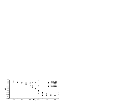
Figure 2: $\langle\varphi\rangle/\pi$ as a function of $a\mu_{I}$ for some different values of $\beta$.

III.1 RW TRANSITION AT IMAGINARY CHEMICAL POTENTIAL

In this section, we present the results of simulation for addressing the $Z(3)$ transition, and the simulation is performed with $\delta\tau=0.02$ for which the acceptance rate is approximately $90-95\%$.

The SU(3) gauge theory with fermions at imaginary $\mu$ has periodicity with period $2\pi T/N_{c}$Roberge:1986mm ; deForcrand:2002ci ; Lombardo . In the high temperature deconfined phase, there is a first order phase transition between different Z(3) sectors, while in the low temperature phase, the transition becomes a crossover at some critical imaginary chemical potential values $\mu_{I}^{c}$ Roberge:1986mm ; deForcrand:2002ci ; Lombardo ,

$$\frac{\mu_{I}^{c}}{T}={\frac{2\pi}{N_{c}}}\left(k+{\frac{1}{2}}\right).$$ (14)

The different Z(3) sectors can be distinguished from each other by the phase of Polyakov loop. In our case, i.e., $N_{c}=3$ and $N_{t}=4$, the first Roberge-Weiss (RW) transition to different Z(3) sectors should appear at $a{\mu_{I}}=\pi/12\approx 0.262$. Because the system will tunnel into the unphysical Z(3) sector above $\mu_{I}/T=\pi/3$, our method is limited up to $\mu_{I}/T=\pi/3$.

Fig. 1 shows the history and probability distribution of the phase $\varphi$ of the Polyakov loop at $a{\mu_{I}}=0.262$, $\kappa=0.165$ and $\beta=5.260$. Figure 2 shows $\varphi/\pi$ as a function of $a\mu_{I}$ at some different values of $\beta$. These indicate that at $a\mu_{I}\approx 0.262$, and $T>T_{E}$ (where $\beta$ is larger than $[5.245,\,5.255]\,$), there is a first order phase transition with $\langle\varphi\rangle$ changing between values of 0 and $-2\pi/3$.

III.2 DECONFINEMENT TRANSITION AT IMAGINARY CHEMICAL POTENTIAL

In order to investigate the deconfinement transition, we take measurements of plaquette variable $P$, Polyakov loop norm $|L|$, chiral condensate ${\bar{\psi}}\psi$ and their susceptibilities $\chi_{P},\,\chi_{|L|},\,\chi_{{\bar{\psi}}\psi}$, and the subtracted chiral condensate $\langle{\bar{\psi}}\psi\rangle_{sub}$ in the first Z(3) sector $a\mu_{I}<(\pi/3N_{t})$ at $a\mu_{I}=0.0,\,\allowbreak 0.10,\,\allowbreak 0.14,\,\allowbreak 0.18,\,\allowbreak 0.21,\,\allowbreak 0.24$ at $\kappa=0.165$ by using the Ferrenberg-Swendsen reweighting method.

The values of $\beta$ at which we make simulations for the Ferrenberg-Swendsen reweighting method and the quark and meson $\pi,\,\rho$ screening mass are presented in Table. 1 except for $a\mu_{I}=0.10,\,0.18$. In order to calculate the subtracted chiral condensate, we must know the quark mass first. At $a\mu_{I}=0.10,\,0.18$, the values of $\beta$ at which we make simulations are the same as those at $a\mu_{I}=0.0$ and we use the quark masses obtained at the four different values of $\beta$ at $a\mu_{I}=0.0$ and $a\mu_{I}=0.21$ as the quark masses at $a\mu_{I}=0.10$ and $a\mu_{I}=0.18$, respectively. For the quark mass differs slightly at the same $\beta$ and different $a\mu_{I}$.

The values of plaquette, Polyakov loop norm, chiral condensate and their susceptibilities are plotted in Fig. 3 and Fig. 4, respectively (we only plot them for three values of $a\mu_{I}$ for clarity). We also display the values of the subtracted chiral condensate for only three values of $a\mu_{I}$ in Fig. 5. These observables at other $a\mu_{I}$’s have similar behavior as shown in Fig. 3,4,5.

Table 1: Results of $\pi,\,\rho$ meson and twice quark screening mass for $N_{f}=2$ on $8^{2}\times 20\times 4$ lattice. The acceptance rates are approximately $75-83\%$, with the exception at $a\mu_{I}=0.24,\,\beta=5.24$, at that point, the acceptance rate is $70\%$.

$a\mu_{I}$	$\beta$	$m_{\pi}a$	$2m_{q}a$	$m_{\rho}a$
0.00	5.195	1.244(2)	0.4193(9)	1.354(2)
	5.215	1.301(2)	0.2550(5)	1.410(1)
	5.235	1.327(2)	0.1893(4)	1.437(1)
	5.255	1.354(2)	0.1386(2)	1.455(1)
0.14	5.195	1.203(2)	0.4542(9)	1.298(2)
	5.215	1.217(2)	0.3286(7)	1.290(2)
	5.235	1.301(2)	0.2024(3)	1.328(2)
	5.255	1.320(2)	0.1546(2)	1.345(2)
0.21	5.195	1.182(3)	0.461(1)	1.274(2)
	5.215	1.140(2)	0.421(1)	1.228(2)
	5.235	1.177(3)	0.2527(7)	1.201(2)
	5.255	1.278(2)	0.1558(3)	1.237(2)
0.24	5.200	1.169(2)	0.456(1)	1.263(2)
	5.220	1.117(3)	0.416(1)	1.211(2)
	5.240	1.098(3)	0.338(1)	1.148(3)
	5.260	1.242(3)	0.1013(2)	1.192(2)

Figure 3: Mean values of the plaquette, the Polyakov loop norm and the chiral condensate at $\kappa=0.165$.

Figure 4: Susceptibilities for the plaquette, the Polyakov loop norm and the chiral condensate at $\kappa=0.165$.

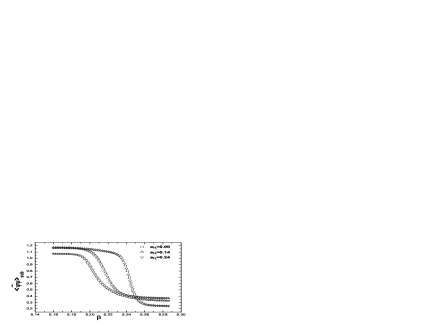
Figure 5: Mean values of the subtracted chiral condensate at $\kappa=0.165$.

From Fig. 3 and Fig. 5, one sees that around the same $\beta$’s, the values of $P,\,|L|,\,{\bar{\psi}}\psi$ and the subtracted chiral condensate $\langle{\bar{\psi}}\psi\rangle_{sub}$ change rapidly and the value of ${\bar{\psi}}\psi$ is larger than that of $\langle{\bar{\psi}}\psi\rangle_{sub}$ at the same $\beta$ and $a\mu_{I}$. Fig. 4 tells that the locations of the peaks for $\chi_{P},\,\allowbreak\chi_{|L|},\,\allowbreak\chi_{{\bar{\psi}}\psi}$ are consistent with each other within errors. We determine the transition points $\beta_{c}(a\mu_{I})$ from the locations of susceptibility peaks, the results are listed in Table. 2.

In Ref. deForcrand:2002ci , it has been established in detail that because the partition function $Z$ as an even function of $a\mu$ leads to an even susceptibility $\chi$, and at the transition points, $\partial\chi/\partial\beta=0$, this expression implicitly defines $\beta_{c}(a\mu)$ as an even function of the real chemical potential $a\mu$ due to implicit function theorem; that when the purely imaginary chemical potential is considered, the considerations are unchanged, so, pseudo-critical line of the transition at imaginary chemical potential is simply the analytic continuation of the pseudo-critical line at real chemical potential; hence that the pseudo-critical transition line at imaginary chemical potential $\beta_{c}(a\mu_{I})$ is an even function of $a\mu_{I}$ and can be fitted well by a polynomial of degree one in $(a\mu_{I})^{2}$ without taking into account the term of degree two in $(a\mu_{I})^{2}$, that is to say:

$$\beta_{c}(a\mu_{I})=c_{0}+c_{1}(a\mu_{I})^{2}+O(a^{4}\mu_{I}^{4}),$$ (15)

After we obtain the expression for $\beta_{c}(a\mu_{I})$ as a polynomial of $(a\mu_{I})^{2}$, we continue back to the real chemical potential and get $\beta_{c}(a\mu)$ as a function of $a\mu$.

We use the least squares method to fit the data in Table 2, the coefficients and $\chi^{2}/dof$ are listed in Table 3. The fitting range and the line are presented in Fig. 6. From Fig. 6, we find that the coefficients of terms in $(a\mu_{I})^{2}$ with higher order than one are difficult to be determined with high precision. From Table 3, we can find that the fitting result from chiral condensate is better than the results from $P$ and $L$, so our choice for the pseudo-critical transition line is:

$$\beta_{c}(a\mu_{I})=5.201(3)+0.722(80)(a\mu_{I})^{2}+O(a^{4}\mu_{I}^{4}).$$ (16)

the errors are the fit errors.

We estimate the pseudo-scalar meson mass $m_{\pi}$, the vector meson mass $m_{\rho}$ and their ratio $m_{\pi}/m_{\rho}$ at our simulation points from the data in Ref. Bitar:1990si . By using the standard quark and gauge action, Bitar et al. found that at $\kappa=0.16,\,\beta=5.28$, $am_{\pi}=1.213\pm 0.004$ and $am_{\rho}=1.287\pm 0.0005$, at $\kappa=0.17,\,\beta=5.12$, $am_{\pi}=1.088\pm 0.003$ and $am_{\rho}=1.210\pm 0.005$. Our critical $\beta$ values range from $\beta=5.199$ to $\beta=5.243$ at $\kappa=0.165$, so we estimate that at the transition points in our simulation, $am_{\pi}$’s are in the interval from $1.213\pm 0.004$ to $1.088\pm 0.003$, $am_{\rho}$’s from $1.287\pm 0.0005$ to $1.210\pm 0.005$, and the ratios of $m_{\pi}/m_{\rho}$ are between $0.943(3)$ and $0.899(4)$.

Table 2: Collection of pseudo-critical transition points at $\kappa=0.165$, determined by locating the peaks of the susceptibilities.

$a\mu_{I}$	0.00	0.10	0.14	0.18	0.21	0.24
$\beta_{C}$ from $\chi_{P}$	5.199(5)	5.208(4)	5.215(7)	5.226(4)	5.233(3)	5.243(3)
$\beta_{C}$ from $\chi_{L}$	5.199(5)	5.209(4)	5.215(5)	5.226(4)	5.233(3)	5.243(3)
$\beta_{C}$ from $\chi_{\bar{\psi}\psi}$	5.200(5)	5.208(4)	5.218(7)	5.226(5)	5.234(4)	5.242(3)

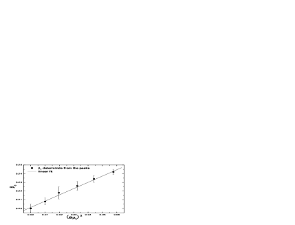
Figure 6: Locations of pseudo critical coupling determined from $\chi_{\bar{\psi}\psi}$, the line shows the fit.

Figure 7: Illustrative figure of transition temperature as a function of $\mu_{B}$. The dotted lines reflect the error on $c_{1}$, the error bar is due to the uncertainty in $T_{c}(0)$.

III.3 DECONFINEMENT TRANSITION AT REAL CHEMICAL POTENTIAL $\mu$

Now it is trivial to get the pseudo-critical line on the $(\mu,T)$ plane. Because $\beta_{c}(a\mu_{I})$ is an analytic function of $a\mu_{I}$deForcrand:2002ci , we can analytically continue from the imaginary chemical potential to the real one. Replacing ${\mu}_{I}$ by $-i{\mu}$ in Eq. (16), we obtain $\beta_{c}({a\mu})$,

$$\beta_{c}(a\mu) = c_{0}-c_{1}(a\mu)^{2}+O(a^{4}\mu^{4})$$ (17)

$$= 5.201(3)-0.722(80)(a\mu)^{2}+O(a^{4}\mu^{4}).$$

To translate our result into physical unit, we use the two loop perturbative solution to the renormalization group equation between the lattice spacing $a$ and $\beta$:

$$a\Lambda_{L} = \exp\bigg{[}-\frac{1}{12b_{0}}\beta+\frac{b_{1}}{2b_{0}^{2}}\ln\left(\frac{1}{6b_{0}}\beta\right)\bigg{]},$$

$$b_{0} = \frac{1}{16\pi^{2}}(11-\frac{2}{3}N_{f}),$$

$$b_{1} = (\frac{1}{16\pi^{2}})^{2}(102-\frac{38}{3}N_{f}).$$ (18)

From this and $T=1/(aN_{t})$, we obtain

$$\frac{T_{c}(\mu)}{T_{c}(0)}=\frac{a(\beta_{c}(0))\Lambda_{L}}{a(\beta_{c}(\mu))\Lambda_{L}}$$ (19)

by replacing $a$ with $1/(N_{t}T_{c})$, it gives:

$$\frac{T_{c}(\mu)}{T_{c}(0)}=\cfrac{\exp\bigg{[}-\cfrac{1}{12b_{0}}c_{0}+\cfrac{b_{1}}{2b_{0}^{2}}\ln\Big{(}\cfrac{1}{6b_{0}}c_{0}\Big{)}\bigg{]}}{\exp\bigg{\{}-\cfrac{1}{12b_{0}}\Big{[}c_{0}-c_{1}(\cfrac{\mu}{N_{t}T_{c}})^{2}\Big{]}+\cfrac{b_{1}}{2b_{0}^{2}}\ln\bigg{[}\cfrac{1}{6b_{0}}\Big{[}c_{0}-c_{1}(\cfrac{\mu}{N_{t}T_{c}})^{2}\Big{]}\bigg{]}\bigg{\}}}.$$ (20)

Expand the right hand side of Eq. (20) as a series of $\mu^{2}$ and neglect the higher order terms , we can obtain the expression of $T_{c}$ as a function of $\mu_{B}^{2}$.

$$\frac{T_{c}(\mu_{B})}{T_{c}(\mu_{B}=0)}=1-0.00722(80)(\frac{\mu_{B}}{T})^{2},$$ (21)

where the baryon chemical potential $\mu_{B}$ is related to the quark chemical potential by $\mu=\mu_{B}/N_{c}$ and the error only reflects the error on $c_{1}$. $T_{c}(\mu_{B}=0)$ is set by the critical temperature for 2-flavor QCD at $\mu_{B}=0$.

Table 3: Coefficients of Eq. (15) by fitting the data in Table. 2

	$c_{0}$	$c_{1}$	$\chi^{2}/dof$
$\beta_{C}$ from $\chi_{P}$	5.200(3)	0.748(79)	0.057
$\beta_{C}$ from $\chi_{L}$	5.201(3)	0.738(78)	0.075
$\beta_{C}$ from $\chi_{\bar{\psi}\psi}$	5.201(3)	0.722(80)	0.104

Recently, Bernard et al.Bernard:2004je studied the transition temperature of 3-flavor, (2+1) flavor QCD, they obtained $T_{c}=169(12)(4)$MeV or $T_{c}=174(11)(4)$MeV for (2+1) flavor. Cheng et al.Cheng:2006qk performed calculation of the transition temperature of (2+1) flavor QCD, and $T_{c}=192(7)(4)$MeV is their result. Karsch, Laermann and Peikert obtained $T_{c}(\mu=0)=173(8)$MeV in the chiral limit for staggered fermionsKarsch . Ali Khan et al. used a renormalization group improved gauge action and clover-improved Wilson quark action to investigate 2-flavor QCD and they obtained $T_{c}(\mu=0)=171(4)$MeVAliKhan:2000iz . The result of Karsch et al. and Ali Khan et al. are consistent with each other. If we take $173(8)$MeV as $T_{c}(\mu_{B}=0)$, then the transition temperature for $N_{f}=2$ is described by a line illustratively plotted in Fig. 7 from which we can see that $T_{c}$ decreases with increasing $\mu_{B}$.

The imaginary chemical potential method is valid in the range $\mu_{B}/T\leq\pi$, and the pseudo-critical $\beta$ is a polynomial of $(a\mu_{I})^{2}$. However, the data in Fig. 6 imply that we can only calculate the first two coefficients of the polynomial with high precision, so the continuation from imaginary chemical potential to real one is restricted in the range of small $a\mu$ and therefore Eq. (21) is valid in the range of small $\mu_{B}$.

III.4 NATURE OF PHASE TRANSITION

In order to determine the nature of the phase transition with imaginary chemical potential, we investigate the history, histogram and finite size scaling of MC simulation at $\kappa=0,\,0.005,\,0.165$. On lattice $8^{3}\times 4,\,12^{3}\times 4,\,16^{3}\times 4$, at $\kappa=0$ which corresponds to quenched limit or pure gauge theory, we find the critical $\beta$ is $5.70$ by determining the location of the peak of $\chi_{|L|}$. The value of $\beta_{c}$ is consistent with the result of Ref. Brown:1988qe ; Boyd:1995zg . We plot the history and histogram of $\langle|L|\rangle$ around critical $\beta_{c}=5.70$ in Fig. 8. From the histogram and MC history of $\langle|L|\rangle$, we see that near $\beta=5.70$, there are two-state signals which are an indication of first order phase transition.

Because at $\kappa=0.0$, quarks have no effect on the system, it is natural that the value of $\beta_{c}$ and the two-state signal are the same for other values of $a\mu_{I}$ in the quenched limit. So we conclude that at other values of $a\mu_{I}$ in the quenched limit, the phase transition is of first order. We also make simulations at $\kappa=0.005$ on lattice $8^{3}\times 4$, the result is presented in Fig. 9 which tells us that for very heavy quarks, the system with imaginary chemical potential has the feature of first order transition.

Figure 8: Time history and histogram of Polyakov loop at $\kappa=0.0$.

Figure 9: Time history and histogram of Polyakov loop norm at $\kappa=0.005$.

In order to estimate the lattice spacing at $\beta=5.70$, we use the results in Ref. Boyd:1995zg from which we know that at $\beta=5.6925(2)$ with the temporal extent $N_{t}=4$ at the infinite volume, $\sqrt{\sigma}a=0.4179(24)$,$\;\sigma$ is the string tension. Using$\sqrt{\sigma}=420\rm{MeV}$, we estimate that the lattice spacing $a\approx 0.995\rm{GeV^{-1}}$.

At $\kappa=0.165,a\mu_{I}=0.24$, the critical $\beta$ is $5.242(3)$ or $5.243(3)$, and $\beta=5.244$ is consistent with them within errors, so at $\beta=5.244$, we can evaluate the spatial dependence of susceptibilities of Polyakov loop norm and its time history and histogram on lattice of spatial size of $8^{3},\,10^{3},\,12^{3},\,14^{3},\,16^{3},\,18^{3},\,20^{3}$ with temporal extent $N_{t}=4$ with acceptance rate $82\%,\,81\%,\,75\%,\,68\%,\,67\%,\,55\%,\,51\%$. We generate 1,000 configurations except on lattice $12^{3}\times 4$ where 2,000 configurations are generated. We present the spatial dependence in Fig. 10 and the time history and histogram on lattice $8^{3}\times 4,\,12^{3}\times 4,\,16^{3}\times 4$ and $20^{3}\times 4$ in Fig. 11.

From Fig. 10 we find that the peak heights of Polyakov loop norm susceptibilities are approximately the same except for spatial volume $12^{3},\,18^{3}$. On lattice $12^{3}\times 4$, as a comparison, we measure $\chi_{|L|}$ after the first 1,000 configurations are produced, we find that $\chi_{|L|}=21.74(9.46)$, while $\chi_{|L|}=16.38(5.47)$ after the statistic is doubled. We can expect that when statistic is large enough, the values of $\chi_{|L|}$ and their errors on lattice $12^{3}\times 4,\,18^{3}\times 4$ will decrease. The history and histogram of Polyakov loop norm plotted in Fig. 11, together with the peak height change with spatial volume, shows that the transition at $a\mu_{I}=0.24$ is a crossover.

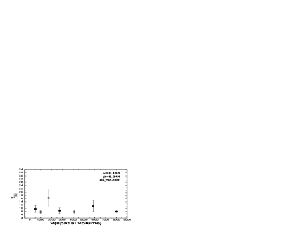
Figure 10: Peak heights of susceptibility of Polyakov loop norm as a function of spatial volume at $a\mu_{I}=0.24$.

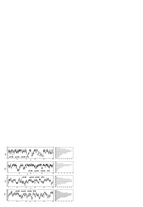
Figure 11: History and histogram of Polyakov loop norm at different spatial volume at $a\mu_{I}=0.24$.

IV DISCUSSION

We have studied the phase diagram of lattice QCD with the two flavor of Wilson fermions through the simulations with imaginary chemical potential. In this case the partition function is periodic in imaginary chemical potential. The different Z(3) sectors are characterized by the phase of Polyakov loop. The Z(3) transition which occurs at $\mu_{I}/T=2\pi(k+1/2)/3$ is of first order in the high temperature phase.

Our study shows that there is a first order phase transition at $\kappa=0$ which corresponds to infinite heavy quarks or the quenched limit, it is natural that the $\beta_{c}$ and hence the critical temperature have no dependence on the chemical potential based on the fact that the fermions have no effect on the system in the quenched limit.

From the experience and literature, we expect that in general, the lighter the quark mass, the stronger effect on the system the fermions have. At $\kappa=0.165$, we observe that the values of $P,\,\allowbreak|L|,\,\allowbreak{\bar{\psi}}\psi$ and subtracted chiral condensate $\langle{\bar{\psi}}\psi\rangle_{sub}$ change rapidly around $\beta_{c}$ and the transition points determined from the susceptibilities of $P,\,\allowbreak|L|,\,\allowbreak{\bar{\psi}}\psi$ coincide with each other within errors. The transition at $\kappa=0.165$ which corresponds to a value of ratio of $m_{\pi}/m_{\rho}$ in the range from $0.943(3)$ to $0.899(4)$ at imaginary chemical potential $a\mu_{I}=0.240$ is a crossover, as discussed in the preceding section.

As for the transition temperature as a function of chemical potential, as discussed in Ref. deForcrand:2002ci , the critical line can be well described by a linear function of $\mu_{B}^{2}$. We make simulation at $\kappa=0.165$ and have not investigated the quark mass dependence of our results. Our central result is represented by Eq. (21) which is qualitatively consistent with yet quantitatively slightly different from that in Ref. deForcrand:2002ci taking errors into account. We think that it is probably because our simulation is at a point of quark mass larger than that in Ref. deForcrand:2002ci . At our simulation points, the ratio of pseudo-scalar meson mass $m_{\pi}$ to vector meson mass $m_{\rho}$ is between $0.943(3)$ and $0.899(4)$, these large ratios mean that the quark mass is large at our simulation points.

In the process of deriving Eq. (21), we use the 2-loop perturbative solution to the renormalization group equation between lattice spacing $a$ and $\beta$. However, in our simulations on lattice with $N_{t}=4$, the values of critical $\beta$ range from $5.199$ to $5.243$, the coupling is so strong that using the 2-loop expression is not a good choice. One would need the non-perturbative expression between $a$ and $\beta$, but it is not determined so far. So we have no choice but to use the 2-loop perturbative expression between $a$ and $\beta$. It is known qualitatively that the lattice spacing varies faster than predicted by the 2-loop perturbative formula at strong couplings. This will have the effect of increasing the curvature in Eq. (21).

Solving Eq. (21), we can obtain the $T(\mu_{B})$ as a function of $\mu_{B}$. We take $173(8)$MeV as $T_{c}(\mu_{B}=0)$ and illustratively plot the transition temperature $T_{c}\rm(MeV)$ versus baryon chemical potential $\mu_{B}\rm(MeV)$ in Fig. 7 from which we find that the transition temperature $T_{c}$ decreases slowly with increasing $\mu_{B}$. This behavior is in accordance with the physical picture. With baryon density increasing, the interaction between quarks and gluons becomes weaker and thus quark and gluon degrees of freedom get more easily excited, therefore, the critical temperature decreases with increasing baryon chemical potential. As discussed in Sec. III.3, Eq. (21) is valid in the range of small $\mu_{B}$.

In order to get the transition occur for small $m_{\pi}/m_{\rho}$ and make the use of 2-loop perturbative relation between lattice spacing $a$ and $\beta$ more reliable, lattices with larger temporal extent $N_{t}$ would be used. The investigation of chemical potential dependence of transition temperature in the chiral limit and quark mass dependence of transition temperature awaits further work. Moreover, how to extract the information about the nature of transition with real chemical potential from the behavior with imaginary chemical potential remains an open question.

- (1) M. G. Alford, K. Rajagopal and F. Wilczek, Phys. Lett. B 422, 247 (1998); R. Rapp, T. Schafer, E. V. Shuryak and M. Velkovsky, Phys. Rev. Lett. 81, 53 (1998); K. Rajagopal, Nucl. Phys. A 661, 150 (1999), and refs. therein.
- (2) P. Hasenfratz and F. Karsch, Phys. Lett. B 125, 308 (1983).
- (3) I. M. Barbour, S. E. Morrison, et al., Nucl. Phys. A (Proc. Suppl.) 60, 220 (1998).
- (4) Z. Fodor and S. D. Katz, Phys. Lett. B 534, 87 (2002); JHEP 0203, 014 (2002).
- (5) C. R. Allton et al., Phys. Rev. D 66, 074507 (2002) [arXiv:hep-lat/0204010].
- (6) P. de Forcrand and O. Philipsen, Nucl. Phys. B 642, 290 (2002).
- (7) M. D’Elia and M. P. Lombardo, Phys. Rev. D 67, 014505 (2003).
- (8) P. de Forcrand and O. Philipsen, Nucl. Phys. B 673, 170 (2003); JHEP 0701, 077 (2007).
- (9) H. Neuberger, Phys. Rev. D 70, 097504 (2004).
- (10) B. Bunk, M. Della Morte, K. Jansen and F. Knechtli, Nucl. Phys. B 697, 343 (2004).
- (11) M. Golterman, Y. Shamir and B. Svetitsky, Phys. Rev. D 74, 071501(R) (2006).
- (12) C. W. Bernard et al., Phys. Rev. D 49, 3574 (1994) [arXiv:hep-lat/9310023].
- (13) C. W. Bernard et al. [MILC Collaboration], Phys. Rev. D 56, 5584 (1997) [arXiv:hep-lat/9703003].
- (14) M. Bochicchio, L. Maiani, G. Martinelli, G. C. Rossi and M. Testa, Nucl. Phys. B 262, 331 (1985).
- (15) M.N. Barber, in Phase Transitions and Critical Phenomena, eds. C. Domb and J.L. Lebowitz (Academic Press, New York, 1983), Vol 8.
- (16) Y. Iwasaki, K. Kanaya, S. Kaya and T. Yoshié, Phys. Rev. Lett. 78, 179 (1997) [arXiv:hep-lat/9609022].
- (17) S. Itoh, Y. Iwasaki, Y. Oyanagi and T. Yoshié, Nucl. Phys. B 274, 33 (1986).
- (18) A. Ali Khan et al. [CP-PACS Collaboration], Phys. Rev. D 63, 034502 (2001) [arXiv:hep-lat/0008011].
- (19) A. M. Ferrenberg and R. H. Swendsen, Phys. Rev. Lett. 63, 1195 (1989).
- (20) S. Gottlieb, W. Liu, D. Toussaint, R. L. Renken and R. L. Sugar, Phys. Rev. D 35, 3972 (1987).
- (21) K. M. Bitar et al., Phys. Rev. D 43, 2396 (1991).
- (22) A. Roberge and N. Weiss, Nucl. Phys. B 275, 734 (1986).
- (23) C. Bernard et al. [MILC Collaboration], Phys. Rev. D 71, 034504 (2005) [arXiv:hep-lat/0405029].
- (24) M. Cheng et al., Phys. Rev. D 74, 054507 (2006) [arXiv:hep-lat/0608013].
- (25) F. Karsch, E. Laermann and A. Peikert, Nucl. Phys. B 605, 579 (2001),
- (26) F. R. Brown, N. H. Christ, Y. F. Deng, M. S. Gao and T. J. Woch, Phys. Rev. Lett. 61 (1988) 2058.
- (27) G. Boyd, J. Engels, F. Karsch, E. Laermann, C. Legeland, M. Lutgemeier and B. Petersson, Phys. Rev. Lett. 75, 4169 (1995) [arXiv:hep-lat/9506025].
- (28) http://physics.utah.edu/~detar/milc/