Light meson masses and non-perturbative renormalisation in 2+1 flavour domain wall QCD

Abstract:

We present results for the light meson masses, the bare strange quark mass and preliminary non-perturbative renormalisation of $B_{K}$ in 2+1 flavour domain wall QCD. The ensembles used were generated with the Iwasaki gauge action and have a volume of $16^{3}\times 32$ with a fifth dimension size of 16 and an inverse lattice spacing of 1.6 GeV. These ensembles have $u$ and $d$ masses as low as one quarter of the strange quark mass. All data were generated jointly by the UKQCD and RBC collaborations on QCDOC machines.

Edinburgh 2006/35
SWAT 05/476
SHEP-0634

1 INTRODUCTION AND SIMULATION PARAMETERS

This work describes results from 2+1 flavour domain wall ensembles with a lattice size of $16^{3}\times 32$ recently generated by the RBC and UKQCD collaborations. The analysis was carried out using the standard domain wall Dirac operator [1] and Pauli-Villars fields with the action introduced in [2]. The configurations were generated with the Iwasaki gauge action [3], using the RHMC algorithm [4, 5] with a trajectory length of 1.0, domain wall height of 1.8, $\beta=2.13$ and a fifth dimension of length 16. Three ensembles were generated with a fixed approximate strange quark mass, $am_{s}=0.04$, and a light isodoublet with masses $am_{ud}$ = 0.01, 0.02 or 0.03. The number of trajectories in each ensemble and the number of configurations used in the analysis are shown in table 1. At present, $24^{3}\times 64$ ensembles with the same parameter values are being generated in order to study finite size effects and to compute a wider range of physical quantities.

In this paper we consider meson correlators with valence quark masses equal to the light isodoublet in the sea, the strange quark mass in the sea and the non-degenerate combinations. To improve our statistics, correlators were oversampled and averaged into bins of size between five and ten, depending on the Monte Carlo time separation between measurements. The binning is consistent with the integrated auto-correlation length for the pseudoscalar meson, which was calculated to be of order 50 trajectories. Multiple sources per configuration and several different types of smearing have also been used to improve the signal. A full correlated analysis was then performed with the binned data as input.

2 RESULTS

2.1 The residual mass

The residual mass, which is a measure of the violation of chiral symmetry due to the finite fifth dimension [1], was calculated from the ratio of the point-split pseudoscalar density, $J_{5}$, at the middle of the fifth dimension, to the pseudoscalar density, $P$, built from the fields on the walls [1]

$$am_{\rm res}=\frac{\Sigma_{\vec{x},\vec{y}}\langle J_{5}(\vec{y},t)P(\vec{x},0)\rangle}{\Sigma_{\vec{x},\vec{y}}\langle P(\vec{y},t)P(\vec{x},0)\rangle}.$$ (1)

A simple unitary linear chiral extrapolation was performed, $am_{\rm res}=A+Bam_{f}$, where $am_{f}$ is the input valence quark mass and the self-consistent value, $am_{\rm res}^{\chi}=\frac{A}{(1+B)}$, was defined to be the residual mass in the chiral limit. The self-consistent value obtained in the chiral limit is given in table 1. This corresponds to a residual mass of 5 MeV.

$V\times L_{s}$	$\frac{am_{ud}}{am_{s}}$	$N_{\rm traj}$	$N_{\rm meas}$	$N_{\rm meas}^{\rm NPR}$	$am_{\rm res}^{\chi}$	$am_{s}$	$am_{PS}$
$16^{3}\times 32\times 16$	0.01/0.04	4000	1400	150			0.245(2)
$16^{3}\times 32\times 16$	0.02/0.04	4000	700	150	0.00308(3)	0.042(2)	0.324(2)
$16^{3}\times 32\times 16$	0.03/0.04	4000	700	150			0.390(2)

Table 1: RHMC 2+1 flavour datasets, the value of the residual mass in the chiral limit, $am_{\rm res}^{\chi}$, the bare strange quark mass and the unitary pseudoscalar meson mass, $am_{PS}$.

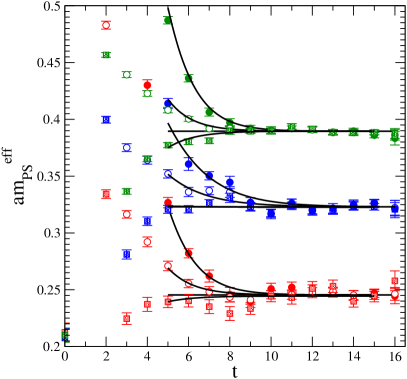
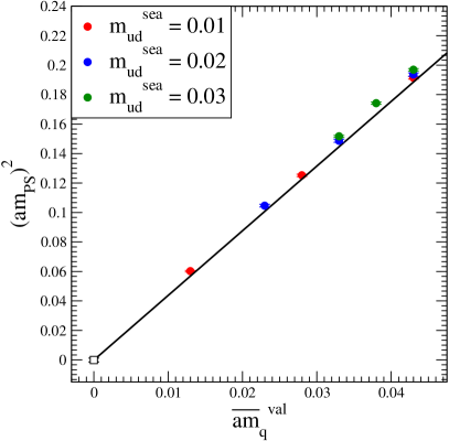
Figure 1: LEFT: Pseudoscalar meson effective masses. Different colours correspond to different quark masses, open, closed and square symbols denote different smearings. Horizontal lines show the fit to the ground state mass while the curved lines result from inputting the fit parameters into equation (2). RIGHT: Chiral extrapolation of the pseudoscalar meson mass against average valence quark mass $\bar{m_{q}}=\left(am_{q_{1}}^{\rm{val}}+am_{q_{2}}^{\rm{val}}\right)/2$. The slope shown comes from parameter $B$ in equation (4) and corresponds to extrapolation to the chiral limit. Different colours denote different light sea quark masses. It may be seen that the sea quark mass dependence, parameter $C$ in equation (4), is very mild.

2.2 Light meson masses

Pseudoscalar and vector meson masses were extracted by performing a simultaneous double cosh fit to the form

$$C_{1}(t) = A_{1}^{G}\left(e^{-m_{G}t}+e^{-m_{G}(T-t)}\right)+A_{1}^{E}\left(e^{-m_{E}t}+e^{-m_{E}(T-t)}\right)$$ (2)

$$C_{2}(t) = A_{2}^{G}\left(e^{-m_{G}t}+e^{-m_{G}(T-t)}\right)+A_{2}^{E}\left(e^{-m_{E}t}+e^{-m_{E}(T-t)}\right)$$

to extract both the ground and first excited states. This helped to remove the systematic error in the choice of fit range due to the excited state. Figure 1 (left) shows typical effective masses for the pseudoscalar mesons.

We set the scale in three ways. Firstly, the lattice spacing was obtained from $m_{\rho}$ in the chiral limit by performing a simple linear unitary chiral extrapolation of the vector meson mass

$$am_{V}=C(am_{q}^{val=sea})+D$$ (3)

where the quark mass, $am_{q}$, was defined by $am_{q}\equiv a(m_{f}+m_{\rm res}^{\chi})$ with $am_{f}$ the input quark mass. Secondly, $r_{0}$ was determined from the quark-antiquark static potential presented in this conference [6], and finally, the method of planes [7] was used. All three methods gave a consistent value for the lattice spacing of $a^{-1}=1.60(3)$ GeV, and therefore a box size of $\sim 2$fm. The lightest pseudoscalar meson has a mass of approximately $390$ MeV.

The non-degenerate pseudoscalar meson masses were chirally extrapolated by fitting both the valence and sea quark mass dependence using the form

$$(am_{PS})^{2}=A+B\left(am_{q_{1}}^{\rm{val}}+am_{q_{2}}^{\rm{val}}\right)+Cam_{q}^{\rm{sea}}.$$ (4)

Figure 1(right) shows the pseudoscalar meson mass squared plotted against the average valence quark mass, $\overline{am_{q}}=(am_{q_{1}}^{\rm{val}}+am_{q_{2}}^{\rm{val}})/2$. The value of $A$ was found to be consistent with zero in good agreement with the residual mass behaving as an additive renormalisation to the input quark mass, $m_{f}$. The normal quark mass, $am_{n}$, was obtained from the physical pion mass by setting $am_{n}=am_{q_{1}}^{\rm{val}}=am_{q_{2}}^{\rm{val}}=am_{q}^{\rm{sea}}$ in equation (4). Similarly, the strange quark mass, $am_{s}$, was obtained from the physical kaon mass by substituting $am_{n}=am_{q_{1}}^{\rm{val}}=am_{q}^{sea}$ and $am_{s}=am_{q_{2}}^{\rm{val}}$. In both cases the scale was taken to be 1.60(3) GeV. The value obtained for the bare strange quark mass (see table 1) is in agreement with the input value of $0.04+am_{\rm{res}}^{\chi}$.

2.3 Non-perturbative renormalisation for $B_{K}$

$B_{K}$ measures the QCD correction to the weak mixing between $K^{0}=(\bar{s}d)$ and $\bar{K^{0}}=(s\bar{d})$ which is an important constraint on the CKM matrix. It is evaluated from the dimensionless ratio of the matrix element of the $\Delta S=2$ operator,

$$\mathcal{O}_{B_{K}}=\mathcal{O}_{VV+AA}=(\bar{s}\gamma_{\mu}d)(\bar{s}\gamma_{\mu}d)+(\bar{s}\gamma_{5}\gamma_{\mu}d)(\bar{s}\gamma_{5}\gamma_{\mu}d)\,,$$ (5)

to its vacuum saturation approximation

$$B_{K}=\frac{\langle\bar{K^{0}}|\mathcal{O}_{B_{K}}|K^{0}\rangle}{\frac{8}{3}m_{K}^{2}f_{K}^{2}}.$$ (6)

Chiral symmetry breaking may cause mixing of the operator $\mathcal{O}_{B_{K}}$ with four other four-quark operators

$${\cal O}_{VV-AA} = (\bar{s}\gamma_{\mu}d)(\bar{s}\gamma_{\mu}d)-(\bar{s}\gamma_{5}\gamma_{\mu}d)(\bar{s}\gamma_{5}\gamma_{\mu}d),$$ (7)

$${\cal O}_{SS\pm PP} = (\bar{s}d)(\bar{s}d)\pm(\bar{s}\gamma_{5}d)(\bar{s}\gamma_{5}d),$$ (8)

$${\cal O}_{TT} = (\bar{s}\sigma_{\mu\nu}d)(\bar{s}\sigma_{\mu\nu}d)\,,$$ (9)

however, the exponentially accurate chiral symmetry afforded by the domain wall fermion formulation should strongly suppress this mixing. In the presence of chiral symmetry breaking the renormalised $B$-parameter, $B_{K}^{\rm(ren)}$, is in principle an admixture of the five lattice $B$-parameters

$$B_{K}^{\rm(ren)}=Z_{VV+AA,VV+AA}/Z_{A}^{2}\cdot B_{K}^{\rm(latt)}+\sum_{i}Z_{VV+AA,i}/Z_{A}^{2}\cdot B_{i}^{\rm(latt)}\,,$$ (10)

for $i\in\{VV-AA,SS\pm PP,TT\}$. It may be observed from figure 2 (left) that the magnitude of the $B$-parameters for the wrong chirality operators are large in comparison with $B^{\rm latt}_{VV+AA}$, the matrix element of interest, and hence the sizes of the mixing coefficients, $Z_{VV+AA,i}$, are crucial.

The renormalisation coefficients are evaluated using the Rome-Southampton method [8] of non-perturbative renormalisation. In Landau gauge, the amputated $n$-point correlation function of the operator of interest, $\Gamma^{(n){\rm latt}}_{\cal O}$, is constructed by applying, at fixed external quark momenta and zero quark mass, the condition

$$Z_{q}^{-n/2}Z_{ij}{\rm P}_{k}\left[\Gamma_{{\cal O}_{j}}^{(n){\rm latt}}(p\ ;\ a^{-1})\right]={\rm P}_{k}\left[\Gamma^{(n){\rm tree}}_{{\cal O}_{i}}\right]\,,$$ (11)

where ${\rm P_{k}}$ represents the application of a particular spin-color projection and a subsequent trace.

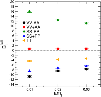
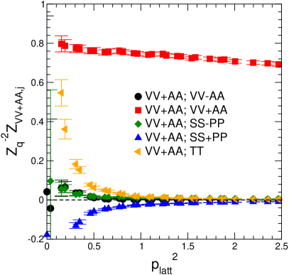
Figure 2: LEFT: B-parameters for $\mathcal{O}_{VV+AA}$, $\mathcal{O}_{VV-AA}$, $\mathcal{O}_{SS+PP}$, $\mathcal{O}_{SS-PP}$ and $\mathcal{O}_{TT}$ as a function of input quark mass, $m_{f}$. RIGHT: Renormalisation factors $Z_{q}^{-2}Z_{VV+AA,j}$ as a function of $p^{2}_{\rm{latt}}$. This demonstrates that the mixing matrix is, in practice, block diagonal with negligible chirality mixing. For each momentum the data has been linearly extrapolated to the chiral limit ($m_{q}\rightarrow 0$).

The set of momenta used to calculate the ratio of renormalisation factors $Z_{Q^{(\Delta S=2)}}/Z_{A}^{2}$ is defined by

$$p_{\rm latt}=\left(\frac{2\pi}{L_{x}}n_{x},\frac{2\pi}{L_{y}}n_{y},\frac{2\pi}{L_{z}}n_{z},\frac{2\pi}{L_{t}}n_{t}\right)$$ (12)

where $L_{x}=L_{y}=L_{z}=16$ and $L_{t}=32$, using 1359 combinations of $(n_{x},n_{y},n_{z},n_{t})$ with $-2\leq n_{x},n_{y},n_{z}\leq 2$ and $-5\leq n_{t}\leq 5$. These are then averaged into 29 combinations of equal $p_{\rm latt}^{2}$. The number of gauge configurations used for the non-perturbative renormalisation is given in table 1.

Results for the elements of the top row of the mixing matrix, $\Lambda_{VV+AA,j}$, $Z_{q}^{2}Z_{VV+AA,j}^{-1}$, versus $p_{\rm latt}^{2}$ are shown in figure 2 (right). It may be seen from the plot that, in the window of momenta for which contributions from both hadronic effects (low momenta) and contributions from discretisation effects (high momenta) are small, the resulting mixing coefficients are small enough that the matrix becomes block diagonal, simplifying the inverse, and hence the wrong chirality operators can be safely neglected. Therefore, we calculate the $B_{K}$ renormalisation factor as $Z_{B_{K}}^{\rm\,RI/MOM}=Z_{VV+AA}/Z_{A}^{2}$. In order to obtain a value for $B_{K}$ in the $\overline{MS}$ scheme at some scale a continuum running/matching calculation was performed following the techniques in [9]. A preliminary value for $Z_{B_{K}}(\overline{MS}$, 2GeV$)$ of 0.90(2) was obtained.

3 SUMMARY

Recent 2+1 flavour simulations using domain wall fermions, the Iwasaki gauge action, three different light isodoublet quark masses and a volume of $16^{3}\times 32$ with a fifth dimension size of 16 have been performed by the RBC and UKQCD collaborations. The chiral symmetry breaking, parameterised by the residual mass, is consistent with a small additive quark mass renormalisation of 5 MeV, which is at an acceptable level with a fifth dimension size of 16. Reasonable signals have been obtained for the pseudoscalar and vector meson masses. These ensembles have a lattice spacing of 1.60(3) GeV and hence the lightest pseudoscalar meson has a mass of approximately 390 MeV. We find that the bare strange quark mass evaluated from the pseudoscalar chiral extrapolation is in good agreement with the input strange quark mass.

The improved chiral symmetry afforded by the domain wall fermion formulation leads to the suppression of mixing with the wrong chirality operators in the calculation of $B_{K}$. This greatly simplifies this calculation and should allow for an accurate determination of the matrix element [10].

References

- [1] V. Furman and Y. Shamir, Nucl. Phys. B439 (1995) 54–78 [hep-lat/9405004].
- [2] P. M. Vranas, Phys. Rev. D57 (1998) 1415–1432 [hep-lat/9705023].
- [3] Y. Iwasaki, UTHEP-118.
- [4] M. A. Clark, A. D. Kennedy and Z. Sroczynski, hep-lat/0409133.
- [5] R. Mawhinney. Production and Properties of 2+1 flavor DWF ensembles, \posPoS(LAT2006)188.
- [6] M. Li, hep-lat/0610106.
- [7] C. R. Allton, V. Gimenez, L. Giusti and F. Rapuano, Nucl. Phys. B489 (1997) 427–452 [hep-lat/9611021].
- [8] G. Martinelli, C. Pittori, C. T. Sachrajda, M. Testa and A. Vladikas, Nucl. Phys. B445 (1995) 81–108 [hep-lat/9411010].
- [9] Y. Aoki et. al., Phys. Rev. D73 (2006) 094507 [hep-lat/0508011].
- [10] S. Cohen. on 2+1 flavor Iwasaki DWF lattices, \posPoS(LAT2006)080.