Nucleon Form Factors: Probing the Chiral Limit

Abstract:

The electromagnetic form factors provide important hints for the internal structure of the nucleon and continue to be of major interest for experimentalists. For an intermediate range of momentum transfers the form factors can be calculated on the lattice. However, reliability of the results is limited by systematic errors due to the required extrapolation to physical quark masses. Chiral effective field theories predict a rather strong quark mass dependence in a range which was yet unaccessible for lattice simulations. We give an update on recent results from the QCDSF collaboration using gauge configurations with $N_{\rm f}=2$, non-perturbatively O(a)-improved Wilson fermions at very small quark masses down to 340 MeV pion mass, where we start to probe the relevant quark mass region.

1 Introduction

In recent years the phenomenological interest in the electromagnetic form factors of the nucleon has revived. This was triggered by the Jefferson Lab polarisation experiments [1, 2] measuring the ratio of the proton electric to magnetic form factors, $\mu^{\rm(p)}G_{e}^{\rm(p)}(Q^{2})/G_{m}^{\rm(p)}(Q^{2})$. From these measurements an unexpected decrease of this ratio has been found, which means that the proton’s electric form factor falls off faster than the magnetic form factor.

Many theoretical calculations have been done to investigate possible interpretations of a decrease of this ratio (see, e.g., [2] for an overview). Lattice techniques allow the calculation of the form factors from first principles. Such calculations do not only yield phenomenologically interesting quantities such as magnetic and electric charge radii and magnetic moments. These techniques also allow, e.g., the investigation of the $Q^{2}$ dependence of the nucleon electromagnetic form factors, which can be compared with experimental results and also helps in understanding the asymptotic behaviour of these form factors.

In practice, the calculation of these form factors on the lattice remains a challenge. In recent years progress has been made to improve control on systematic errors which are related to the fact that the calculations are performed on finite volumes, at finite lattice spacings and at quark masses which are still relatively large. For making reliable predictions at physical quark masses it turned out that numerical results at smaller quark masses are crucial. With recent advances in computing power available to lattice QCD calculations and the speed-up of algorithms for simulating dynamical fermions it is now possible to reach much smaller quark masses with pseudoscalar masses in the range of 300 MeV.

2 Calculation details

In this talk we present results obtained on configurations with two mass degenerate flavours of non-perturbatively $O(a)$-improved Wilson fermions. We choose Wilson glue for the gauge action. To scale the lattice results for different $\beta$ and $\kappa_{\rm sea}$ we use the Sommer parameter $r_{0}(\beta,\kappa_{\rm sea})/a$ and the conversion factor $r_{0}=0.467\;{\rm fm}$ to translate our results into physical units.

The form factors are obtained from the standard decomposition of the nucleon electromagnetic matrix elements

$$\langle p^{\prime},s^{\prime}|J^{\mu}|p,s\rangle=\overline{u}(p^{\prime},s^{\prime})\left[\gamma_{\mu}F_{1}(Q^{2})+i\sigma^{\mu\nu}\frac{q_{\nu}}{2M_{N}}F_{2}(Q^{2})\right]u(p,s),$$ (1)

where $p$ ($s$) and $p^{\prime}$ ($s^{\prime}$) denote initial and final momenta (spins), $q=p^{\prime}-p$ the momentum transfer (with $Q^{2}=-q^{2}$) and $M_{N}$ the nucleon mass. By calculating the matrix elements on the l.h.s. and the nucleon mass we obtain the Dirac form factor $F_{1}(Q^{2})$ and Pauli form factor $F_{2}(Q^{2})$.

The nucleon matrix elements are extracted from ratios of three- and two-point functions:

$$R(t,\tau,\vec{p}\,^{\prime},\vec{p}\,)=\frac{C_{3}(t,\tau,\vec{p}\,^{\prime},\vec{p}\,)}{C_{2}(t,\vec{p}\,^{\prime})}\times\left[\frac{C_{2}(\tau,\vec{p}\,^{\prime})C_{2}(t,\vec{p}\,^{\prime})C_{2}(t-\tau,\vec{p}\,)}{C_{2}(\tau,\vec{p}\,)C_{2}(t,\vec{p}\,)C_{2}(t-\tau,\vec{p}\,^{\prime})}\right]^{1/2}.$$ (2)

Here $t$ denotes the location of the sink. Assuming the source being located at time slice $0$, we expect an plateau for $0\ll\tau\ll t$ (source and sink are separated by a distance of $\sim 1.1$ fm). For further details see [3]. We use three different polarisations $\Gamma_{\rm unpol}=\frac{1}{2}(1+\gamma_{4})$, $\Gamma_{1}=\frac{1}{2}(1+\gamma_{4})\,i\gamma_{5}\gamma_{1}$, $\Gamma_{2}=\frac{1}{2}(1+\gamma_{4})\,i\gamma_{5}\gamma_{2}$ as well as three different sink momenta $\vec{p}_{0}=(0,0,0)$, $\vec{p}_{1}=(p,0,0)$, $\vec{p}_{2}=(0,p,0)$ (where $p=2\pi/L_{S}$). 17 different choices for the momentum transfer $\vec{q}$ have been used. Due to statistical fluctuations the operand of the square root in Eq. (2) may become negative. Results for which this happens are discarded from the consecutive analysis steps.

We use the local vector current, which needs to be renormalised and improved:

$$V_{\mu}=Z_{\rm V}(1+b_{\rm V}am_{q})\left[\bar{q}\gamma_{\mu}q+{\mathrm{i}}c_{\rm V}a\partial_{\lambda}(\bar{q}\sigma_{\mu\lambda}q)\right].$$ (3)

The renormalisation coefficient $Z_{\rm V}$ and the parameter $b_{\rm V}$ have been determined non-perturbatively [4]. The improvement coefficient $c_{\rm V}$ is only known perturbatively. However, since this coefficient is expected to be a small number and because the improvement term was found to be small in the quenched approximation [5], we will ignore the improvement of the operator.

In the following we will consider the iso-vector, iso-scalar and the proton form factors. The latter two might receive contributions from quark-line disconnected terms, which are notoriously hard to calculate on the lattice and will not be considered here.

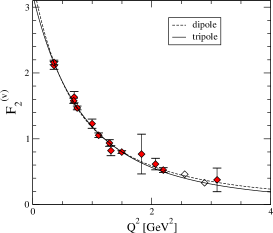
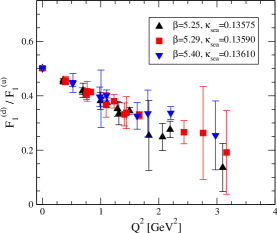
Figure 1: The iso-vector Pauli form factor radius at $(\beta,\kappa_{\rm sea})=(5.25,0.13575)$ (left plot) and the ratio of the iso-vector $d$- and $u$-flavour Dirac form factors (right) as a function of $Q^{2}$. In the right plot we show results for similar $m_{\rm PS}\simeq 400\;{\rm MeV}$ but different lattice spacings.

3 Parameterisation and $Q^{2}$ dependence

First we will investigate the $Q^{2}$ dependence of the Dirac and Pauli form factors. Both lattice and experimental data can be reasonably well parametrised by a pole ansatz

$$F_{i}(Q^{2})=\frac{F_{i}(0)}{(1+Q^{2}/M_{i}^{2})^{p}}.\vspace*{-1mm}$$ (4)

From naive dimensional counting one would expect the Dirac and Pauli form factors to scale differently, i.e. $F_{1}\propto Q^{-4}$ and $F_{2}\propto Q^{-6}$, which corresponds to $p=2$ and $p=3$, respectively. Experimental data as well as theoretical calculations indicate deviations from this naive picture. For instance, the JLab results for $\sqrt{Q^{2}}F_{2}^{\rm(p)}(Q^{2})/F_{1}^{\rm(p)}(Q^{2})$ were found to be surprisingly flat. A perturbative QCD analysis of the Pauli and Dirac form factors predicts the ratio

$$(Q^{2}/log^{2+8/(9\beta)}Q^{2}/\Lambda^{2})F_{2}(Q^{2})/F_{1}(Q^{2})$$ (5)

(with $\beta=11-2N_{\rm f}/3$) to scale as a constant [6]. In an investigation of the $Q^{2}$ dependence of the experimental nucleon form factor data using empirical parameterisations, Diehl and collaborators found indications for the form factor scaling to be flavour dependent [7]. By comparing the Dirac form factor results for proton and nucleon they found the flavour contribution $F_{1}^{\rm(d)}(Q^{2})$ to decrease faster with $Q^{2}$ than $F_{1}^{\rm(u)}(Q^{2})$.

From a first inspection of the lattice results one finds that the effects from changing $p$ in Eq. (4) are small with respect to the statistical errors. In Fig. 1 (left plot) we show the results of a fit to $F_{2}^{\rm(v)}$ for one particular data set using $p=2$ and $3$. It is clear that it is difficult to obtain lattice data with high enough precision over a large enough range of $Q^{2}$ values to distinguish between a dipole or tripole behaviour. It may, however, be instructive to consider ratios of form factors in order to reveal significant deviations from the naive scaling hypothesis. In the right plot of Fig. 1 we show the ratio $F_{1}^{\rm(d)}/F_{1}^{\rm(u)}$ and find that it does not scale as a constant. This is consistent with the observation by Diehl et al. We should however emphasize that we are ignoring possible contributions from disconnected terms.

Based on the above observation we perform fits to the Dirac and Pauli form factors for each flavour separately using the ansatz Eq. (4). To eventually decide which $p$ should be used, we perform these fits for various $1.5\lesssim p\lesssim 4$ and search for the “optimal” $p$ for which $\chi^{2}/\mathrm{d.o.f.}$ becomes minimal. We observe strong variations of the resulting “optimal” $p$ for data sets which differ in ($\beta$,$\kappa_{\rm sea}$,$\kappa_{\rm val}$). However, we nevertheless see clear trends. In case of the $u$-flavour Dirac form factor $F_{1}^{\rm(u)}(Q^{2})$ we find for most data sets $p$ to be close to 2. On the other hand, for the other form factors $F_{1}^{\rm(d)}(Q^{2})$, $F_{2}^{\rm(u)}(Q^{2})$ and $F_{2}^{\rm(d)}(Q^{2})$ we typically get $p\simeq 3$.

4 Form factor radii and magnetic moments

From the fits to Eq. (4) we obtain the form factors at zero momentum transfer $F_{i}(0)$ and the di- or tripole masses $M_{i}$. Equivalently, we can use the same fit to obtain the form factor radii $r_{i}$ and the magnetic moment $\mu$. These quantities are defined as follows:

$$F_{i}(Q^{2}) = F_{i}(0)\left[1-\frac{1}{6}\;{r_{i}^{2}}Q^{2}+{\mathcal{O}}(Q^{4})\right],$$ (6)

$$\mu = F_{1}(0)+F_{2}(0).$$ (7)

From the magnetic moment we can calculate the anomalous magnetic moment, e.g. $\kappa^{\rm(v)}=\mu^{\rm(v)}-1$. For comparison with phenomenological results we use the normalised anomalous magnetic moment, e.g. $\kappa^{\rm(v){\rm norm}}=\kappa^{\rm(v)}\;m_{\rm N}(m_{\pi})/m_{\rm N}(m_{\rm PS})$, where $m_{\rm N}(m_{\rm PS})$ refers to the nucleon mass calculated on the lattice at the quark mass corresponding to the pseudoscalar mass $m_{\rm PS}$ and $m_{\rm N}(m_{\pi})$ the experimental value of the nucleon mass.

In Fig. 2 we show results for $M_{1}^{\rm(v)}$ and $F_{2}^{\rm(v)}(0)$ as a function of $m_{\rm PS}^{2}$ which have been calculated for different values of the gauge coupling $\beta$ and various sea quark masses. These results seem to lie on a universal curve, which indicates that discretisation errors are small. In the following we will consider them as negligible compared to the statistical errors. We furthermore observe that the iso-vector anomalous magnetic moments and di-/tripole masses show a linear quark mass dependence for a very large range of quark masses. However, using an ansatz linear in $(r_{0}m_{\rm PS})^{2}$ to extrapolate our results to the physical point, we obtain values which differ significantly from those extracted from experiment. This is consistent with calculations based on a chiral effective field theory (ChEFT) that includes nucleons, pions and delta resonances as explicit degrees of freedom [9, 3, 8]. These calculations predict for the iso-vector form factor radii and the iso-vector anomalous magnetic moment a strong quark mass dependence in the small quark mass region. This region is just starting to become accessible for simulations with dynamical Wilson quarks.

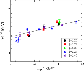
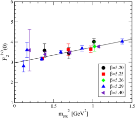
Figure 2: The iso-vector Dirac form factor dipole mass (left plot) and the iso-vector Pauli form factor at zero momentum transfer (right plot) as a function of $m_{\rm PS}^{2}$.

In the left plot of Fig. 3 we compare the lattice results for the iso-vector Dirac form factor radius with the following result from ChEFT, where we used the same phenomenological parameters as in [3]:

$$\left(r_{1}^{\rm(v)}\right)^{2} = -\frac{1}{(4\pi F_{\pi})^{2}}\left\{1+7g_{A}^{2}+\left(10g_{A}^{2}+2\right)\log\left[\frac{m_{\rm PS}}{\lambda}\right]\right\}$$

$$+\frac{{c_{A}}^{2}}{54\pi^{2}F_{\pi}^{2}}\Bigg{\{}26+30\log\left[\frac{m_{\rm PS}}{\lambda}\right]+30\frac{\Delta}{\sqrt{\Delta^{2}-m_{\rm PS}^{2}}}\log\left[\frac{\Delta}{m_{\rm PS}}+\sqrt{\frac{\Delta^{2}}{m_{\rm PS}^{2}}-1}\right]\Bigg{\}}.$$

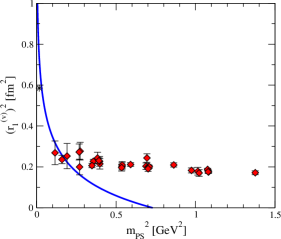
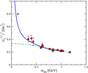
Figure 3: Lattice results for the Dirac (left) and Pauli (right) radii. The solid lines show the ChEFT results given in Eqs. (4.3) and (4.4). Note that the left curve is not based on a fit. In the right-hand plot the dashed line is the result of a fit to the tripole masses linear in $(r_{0}m_{\rm PS})^{2}$. The star denotes the experimental value.

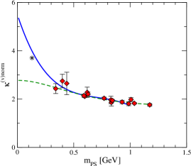
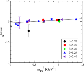
Figure 4: Lattice results for the iso-vector (left) and iso-scalar (right) anomalous magnetic moment. The solid lines in the left plot show the result from a fit to the ChEFT expression in Eq. (4.5). In the right-hand plot an ansatz linear in $(r_{0}m_{\rm PS})^{2}$ has been used to fit the data. The star denotes the phenomenological value.

For the iso-vector Pauli form factor, $r_{2}^{\rm(v)}$, and the anomalous magnetic moment, $\kappa^{\rm(v)}$, we performed a combined fit of the lattice results to the following expressions from ChEFT:

$$\left(r_{2}^{\rm(v)}\right)^{2} = \frac{{g_{A}}^{2}{M_{N}}}{8{F_{\pi}}^{2}\kappa^{\rm(v)}(m_{\rm PS})\pi m_{\rm PS}}+$$

$$\frac{{c_{A}}^{2}M_{N}}{9F_{\pi}^{2}\kappa^{\rm(v)}(m_{\rm PS})\pi^{2}\sqrt{{\Delta}^{2}-m_{\pi}^{2}}}\log\left[\frac{\Delta}{m_{\rm PS}}+\sqrt{\frac{\Delta^{2}}{m_{\pi}^{2}}-1}\right]+\frac{24M_{N}}{\kappa^{\rm(v)}(m_{\rm PS})}\,{B_{c2}},$$

$$\kappa^{\rm(v)}(m_{\rm PS}) = {\kappa^{{\rm(v)}0}}-\frac{{g_{A}}^{2}\,m_{\rm PS}{M_{N}}}{4\pi{F_{\pi}}^{2}}+\frac{2{c_{A}}^{2}{\Delta}M_{N}}{9\pi^{2}F_{\pi}^{2}}\left\{\sqrt{1-\frac{m_{\rm PS}^{2}}{\Delta^{2}}}\log R(m_{\rm PS})+\log\left[\frac{m_{\rm PS}}{2\Delta}\right]\right\}$$

$$-8{E_{1}^{(r)}(\lambda)}M_{N}m_{\rm PS}^{2}+\frac{4c_{A}{c_{V}}g_{A}M_{N}m_{\rm PS}^{2}}{9\pi^{2}F_{\pi}^{2}}\log\left[\frac{2\Delta}{\lambda}\right]+\frac{4c_{A}c_{V}g_{A}M_{N}m_{\rm PS}^{3}}{27\pi F_{\pi}^{2}\Delta}$$

$$-\frac{8c_{A}c_{V}g_{A}\Delta^{2}M_{N}}{27\pi^{2}F_{\pi}^{2}}\Bigg{\{}\left(1-\frac{m_{\rm PS}^{2}}{\Delta^{2}}\right)^{3/2}\log R(m_{\rm PS})+\left(1-\frac{3m_{\rm PS}^{2}}{2\Delta^{2}}\right)\log\left[\frac{m_{\rm PS}}{2\Delta}\right]\Bigg{\}}.$$

Here we keep the chiral limit of the anomalous magnetic moment $\kappa^{{\rm(v)}0}$, the iso-vector $N$-$\Delta$ coupling $c_{V}$ and the ChEFT parameters $B_{c2}$ and $E_{1}^{(r)}$ as free parameters. The result of this fit is displayed in the right plot of Fig. 3 for $(r_{2}^{(v)})^{2}$ and the left plot of Fig. 4 for $\kappa^{(v)}$ together with the lattice data and phenomenological results at $m_{\rm PS}=m_{\pi}$.

The lattice data for the Dirac radius do not seem to agree well with the ChEFT result. Since it is not clear up to which quark masses the ChEFT expression is valid, results at even smaller quark masses will be needed to actually clarify this issue. For both the Pauli radius and the anomalous magnetic moment the lattice and ChEFT results look consistent. It is somewhat surprising that this seems to hold also for rather heavy quarks. From our preliminary results at very low quark masses we see first indications for the Pauli radius to bend towards the phenomenogical value.

Finally, in the right plot of Fig. 4, we show our results for the iso-scalar form factor. From ChEFT a linear quark mass dependence is expected, which is fully consistent with our lattice calculations.

5 Conclusions

We have presented the current status of the calculation of the electromagnetic form factors of the nucleon by the QCDSF collaboration. At the currently achieved level of statistical errors, still large uncertainties remain for the parameterisation of the form factor results. However, qualitative agreement with the experimental data has been found, e.g. the flavour dependence of the Dirac form factor $F_{1}$. As new configurations at very small quark masses are starting to become available, we are improving our control on the extrapolation of the lattice results towards the chiral limit. We have found first indications for strong effects at small quark masses, which have been predicted by ChEFT calculations. However, results at even lower quark masses with higher statistics will be required in order to confirm these predictions.

References

- [1] M. K. Jones et al. [Jefferson Lab Hall A Collaboration], Phys. Rev. Lett. 84 (2000) 1398 [nucl-ex/9910005]; O. Gayou et al. [Jefferson Lab Hall A Collaboration], Phys. Rev. Lett. 88 (2002) 092301 [arXiv:nucl-ex/0111010].
- [2] V. Punjabi et al. [Jefferson Lab Hall A Collaboration], Phys. Rev. C 71 (2005) 055202 [Erratum-ibid. C 71 (2005) 069902] [arXiv:nucl-ex/0501018].
- [3] M. Göckeler et al. [QCDSF Collaboration], Phys. Rev. D 71 (2005) 034508 [arXiv:hep-lat/0303019].
- [4] T. Bakeyev et al. [QCDSF Collaboration], Phys. Lett. B 580 (2004) 197 [arXiv:hep-lat/0305014].
- [5] S. Capitani et al., Nucl. Phys. Proc. Suppl. 73 (1999) 294 [arXiv:hep-lat/9809172].
- [6] A. V. Belitsky et al., Phys. Rev. Lett. 91, 092003 (2003) [arXiv:hep-ph/0212351].
- [7] M. Diehl et al., Eur. Phys. J. C 39 (2005) 1 [arXiv:hep-ph/0408173].
- [8] D. B. Leinweber et al., Phys. Rev. Lett. 86, 5011 (2001) [arXiv:hep-ph/0101211].
- [9] T. R. Hemmert and W. Weise, Eur. Phys. J. A 15 (2002) 487 [arXiv:hep-lat/0204005].
- [10] C. R. Allton et al., Phys. Rev. D 65 (2002) 054502 [arXiv:hep-lat/0107021].