Quark number susceptibility of high temperature QCD

Abstract:

We use three dimensional reduced effective field theory (EQCD) and lattice calculations to determine the quark number susceptibility of QCD at high temperature. We find our results to agree well with known perturbative expansion as well as with other lattice data.

CERN-PH-TH/2006-209

1 Introduction

A dimensionally reduced effective theory is, by now, a well-established and powerful tool for studying high-temperature QCD both perturbatively and non-perturbatively. At high enough temperatures the QCD coupling becomes small, and perturbative methods can be safely applied to hard ($\sim T$) modes. The fact that high-temperature QCD can be reduced to 3d effective theory can be understood by considering an Euclidean finite-$T$ propagator

$$\frac{1}{{\boldmath p}^{2}+\omega^{2}_{n}+m^{2}},$$ (1)

where $\omega_{n}^{b}=2n\pi T$ for bosons and $\omega_{n}^{f}=(2n+1)\pi T$ for fermions. Thus, only static $n=0$ bosonic modes remain “light” at high temperatures, and the heavy $n\neq 0$ bosonic and all fermionic modes can be integrated perturbatively [1, 2, 3, 4]. The result is an effective 3d theory of full QCD, electrostatic QCD (EQCD) [11]. An essential feature of the effective theory is that it fully includes the perturbatively problematic soft ($\sim gT$) and ultrasoft ($\sim g^{2}T$) scales of the original theory; only perturbatively well-controlled hard scales ($\sim T$) are integrated over.

EQCD offers a good starting point both for perturbative calculations [5, 6, 7] and non-perturbative lattice simulations. In the latter case, EQCD offers an interesting alternative to standard high-temperature lattice simulations: above all, the effective theory is purely bosonic and only 3-dimensional, making it much cheaper to simulate. The theory is superrenormalizable, which renders the continuum limit particularly transparent; it also enables simulations at arbitrarily large temperatures. On the other hand, the effective theory cannot be used to study the QCD phase transition: at too low $T$ QCD becomes strongly coupled and the perturbative derivation of EQCD fails. Nevertheless, the theory has been found to work well down to temperatures $T\sim 1.5-3\,T_{c}$, depending on observable used. Lattice simulations of EQCD have been used to calculate QCD pressure at high T [8], spatial string tension [9], and spatial screening lengths [10]. Here we measure the quark number susceptibility, and compare the result to both perturbative and 4d lattice results.

2 Susceptibility in electrostatic QCD

EQCD is defined by the action

$$S_{\textrm{E}} = \int\textrm{d}^{3}x\mathcal{L}_{\textrm{E}}$$

$$\mathcal{L}_{\textrm{E}} = \frac{1}{2}\textrm{Tr}[F_{ij}^{2}]+\textrm{Tr}[D_{i},A_{0}]^{2}+m_{3}^{2}\textrm{Tr}[A_{0}^{2}]+i\gamma_{3}\textrm{Tr}[A_{0}^{3}]+\lambda_{3}(\textrm{Tr}[A_{0}^{2}])^{2},$$ (2)

where $F_{ij}=\partial_{i}A_{j}-\partial_{j}A_{i}+ig_{3}[A_{i},A_{j}]$ and $D_{i}=\partial_{i}+ig_{3}A_{i}$. $F_{ij}$, $A_{i}$ and $A_{0}$ are traceless $3\times 3$ Hermitean matrices ($A_{0}=A_{0}^{a}T_{a}$, etc). Coupling and mass parameters $g_{3}$, $m_{3}$, $\gamma_{3}$ and $\lambda_{3}$ are defined by the physical 4d temperature, renormalization scale $\Lambda_{\overline{\textrm{MS}}}$, chemical potential $\mu$ and the number of massless fermions. It is convenient to use the dimensionless ratios

$$y=\frac{m_{3}^{2}}{g_{3}^{4}},\;\;x=\frac{\lambda_{3}}{g_{3}^{2}},\;\;z=\frac{\gamma_{3}}{g_{3}^{3}},$$ (3)

which determine the physical properties of EQCD. The $\mu$-dependence of the parameters is, at 1-loop level,

$$y=y_{\mu=0}\left(1+\sum_{f}\bar{\mu}_{f}^{2}\frac{3}{2N_{\textrm{c}}+N_{\textrm{f}}}\right),~{}~{}~{}~{}~{}~{}z=\sum_{f}\frac{\bar{\mu}_{f}}{3\pi},~{}~{}~{}~{}~{}~{}x=x_{\mu=0}\,,$$ (4)

where $\bar{\mu}=\mu/(\pi T)$ and the $\mu=0$ expressions can be found in ref. [11]. The two loop corrections have been calculated in ref. [10], but the effects remain in practice negligible.

The quantity we are interested in is the quark number susceptibility, which we calculate over one flavor $u$ only, can be defined in EQCD as

$$\chi_{3}=\frac{1}{V}\frac{\partial^{2}}{\partial\mu_{u}^{2}}\ln{\cal Z}=\frac{1}{V}\frac{\partial^{2}}{\partial\mu_{u}^{2}}\ln\int\mathcal{D}A_{k}A_{0}\exp\left(-S_{\textrm{E}}\right)$$ (5)

Substituting $S_{\textrm{E}}$ from (2) we arrive at equation

$$\chi_{3} = -\frac{6}{2N_{c}+N_{f}}\,y_{\mu=0}\,\langle\textrm{Tr}A_{0}^{2}\rangle+V\frac{N_{f}^{2}}{9\pi^{2}}\langle(\textrm{Tr}A_{0}^{3})^{2}\rangle$$ (6)

$$+V\frac{9N_{f}^{2}}{(2N_{c}+N_{f})^{2}}\bar{\mu}^{2}\,y_{\mu=0}^{2}\,\left(\langle(\textrm{Tr}A_{0}^{2})^{2}\rangle-\langle\textrm{Tr}A_{0}^{2}\rangle^{2}\right)$$

Thus, the quark number susceptibility is obtained by measuring the condensates $\langle TrA_{0}^{2}\rangle$, $\langle(\textrm{Tr}A_{0}^{2})^{2}\rangle$ and $\langle(\textrm{Tr}A_{0}^{3})^{2}\rangle$ on the lattice. Due to the superrenormalizable nature of the theory, measurements can be rigorously converted to $\overline{\textrm{MS}}$ scheme in the lattice continuum limit; because $\overline{\textrm{MS}}$ was used in in the perturbative matching to 4d QCD, this also allows us to compare to 4d results. For example, the continuum limit for the $\langle[TrA_{0}^{3}]^{2}\rangle$ is

$$V\langle[\textrm{Tr}A_{0}^{3}/g_{3}^{3}]^{2}\rangle_{\overline{\textrm{MS}}} = \lim_{\beta\rightarrow\infty}\left\{V\langle[\textrm{Tr}A_{0}^{3}/g_{3}^{3}]^{2}]\rangle_{a}-\frac{5}{16\pi^{2}}\left[\ln\beta+0.08848010\right]\right\},$$ (7)

where $\beta\equiv\frac{2N_{\textrm{c}}}{ag_{3}^{2}}$ is the lattice coupling constant. Continuum limits for $\langle TrA_{0}^{2}\rangle$ and $\langle(\textrm{Tr}A_{0}^{2})^{2}\rangle$ are given in [11]. The relation between $\chi_{3}$ and the true 4d susceptibility is

$$\chi=\frac{g_{3}^{6}}{T^{3}}\chi_{3}+\frac{\partial^{2}}{\partial\mu_{u}^{2}}\Delta p,$$ (8)

where $\Delta p=p_{\textrm{QCD}}-p_{\textrm{3d}}$ is the perturbative 3d$\rightarrow$4d matching coefficient, and can be found in [6].

3 Lattice measurements

Lattice simulations were carried out for $N_{\textrm{f}}=2$. We used large lattice sizes $V=140^{3},200^{3}$ and values of $\beta=$32, 40, 67, 80, 120. The volumes are large enough so that the remaining (exponential) finite volume effects are safely below our statistical accuracy; for a detailed analysis in a related theory see [12].

For each value of $\beta$ we did simulations with values of $y=6.62,\;5.31,\;4.00,\;3,09,\;2.02,\;1.18$, $0.71,$ and $0.45$. The simulations have been carried out for $\mu=0$, and to obtain the susceptibility, one needs measurements of $\langle\textrm{Tr}A_{0}^{2}\rangle$ and $\langle(\textrm{Tr}A_{0}^{3})^{2}\rangle$.

The standard procedure of doing continuum extrapolation is to fit a polynomial to the divergence subtracted lattice data. However, in EQCD the divergent lattice contributions contain also terms of the form $\beta\log(\beta)$ and such terms could also arise in terms $\sim a\sim 1/\beta$. Therefore, we do continuum extrapolation in two ways; we use a second order polynomial

$$c_{1}+\frac{c_{2}}{\beta}+\frac{c_{3}}{\beta^{2}},$$ (9)

and a fitting function of the form

$$c_{1}+\frac{c_{2}}{\beta}+{\frac{c_{2}^{\prime}}{\beta}\log(\beta)}+\frac{c_{3}}{\beta^{2}}.$$ (10)

The Fig. 1 demonstrates the differences between different continuum extrapolations for $\langle\textrm{Tr}A_{0}^{2}\rangle$. The extrapolations done using (10) have excellent $\chi^{2}/$dof, and we shall use this form henceforth. The full continuum extrapolations are shown in Fig. 2. We note that the detailed form of the fitting function is significant for our results; thus, knowledge of the true $1/\beta$ coefficient is highly desirable. There is an ongoing calculation of this term using stochastic perturbation theory [13], which will hopefully confirm our result.

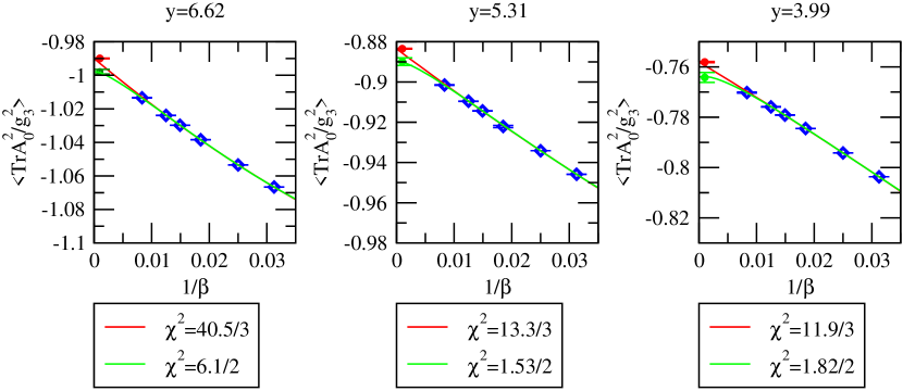
Figure 1: Difference of continuum extrapolations with and without the log-term. The solid line is a fit $c_{1}+\frac{c_{2}}{\beta}+\frac{c_{3}}{\beta^{2}}$ and the dashed line $c_{1}+\frac{c_{2}}{\beta}+{\frac{c_{2}^{\prime}}{\beta}\log(\beta)}+\frac{c_{3}}{\beta^{2}}$.

The contributions of $\langle(\textrm{Tr}A_{0}^{3})^{2}\rangle$ to susceptibility are numerically much smaller than that of $\langle\textrm{Tr}A_{0}^{2}\rangle$. The measurements of $\langle(\textrm{Tr}A_{0}^{3})^{2}\rangle$ are not accurate enough to distinguish between extrapolations (9) and (10), and the choice is not significant for the final results. Hence we use the second order function in Fig. 2.

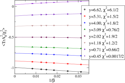
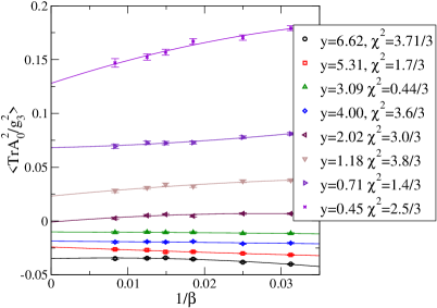
Figure 2: Continuum limits of $\langle\textrm{Tr}A_{0}^{2}\rangle$ and $\langle(\textrm{Tr}A_{0}^{3})^{2}\rangle$ at different values of $y$.

The continuum extrapolated results are shown in Fig. 3, as a function of the parameter $y(T)$. The result agrees very well with the perturbative susceptibility derived in ref. [14]. The perturbative result has the form:

$$\chi_{\textrm{pert}}=a_{1}y^{3/2}+a_{2}y+a_{3}y^{1/2}+a_{4}$$ (11)

where $a_{i}$ are functions of $x$ and $z$. On the right panel we show the difference between the perturbative result and the lattice measurement. Because the lattice measurement (in the continuum limit) fully includes perturbative contributions, we expect the difference to behave as $O(y^{-1/2})$. This is the case when continuum extrapolation is performed using Eq. (10); the extrapolation (9) diverges from perturbative result as $y\rightarrow\infty$, which is inconsistent. This also motivates the use of (10) as continuum extrapolation.

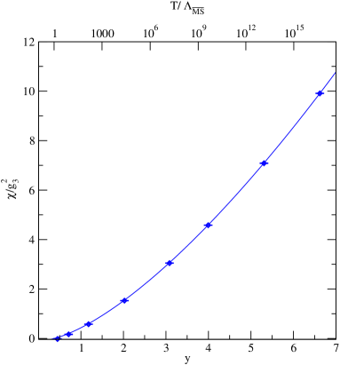
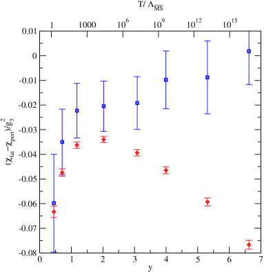
Figure 3: Left: the susceptibility as a function of $y$ and $T/\Lambda_{\overline{\textrm{MS}}}$. The solid line is the perturbative prediction. Right: the difference between the perturbation theory and lattice results. Points denoted by squares are obtained from logarithmic continuum extrapolation and diamonds from polynomial extrapolation; the former one has expected behavior as $y\rightarrow\infty$.

In Fig. 4 we show the susceptibility in 4d units, transformed using Eq. (8), and compare the result to 4d $N_{\textrm{f}}=2$ staggered fermion lattice simulations [16, 17]. Here we use the ratio $T_{c}/\Lambda_{\overline{\textrm{MS}}}=0.49$ [18]. We can observe that our results agree very well with 4d simulations and with perturbation theory. Indeed, the difference between EQCD measurements and perturbative results are all but invisible on the scale of the plot, possibly excluding the lowest temperature data.

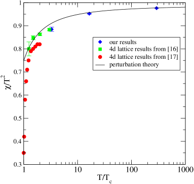
Figure 4: The quark number susceptibility in 4d units. Our results are shown with diamonds, only 3 points fit in the temperature range shown. The results agree very well with 4d lattice simulation results [16, 17].

4 Conclusions and Outlook

We have measured the quark number susceptibility in dimensionally reduced effective theory of high-$T$ QCD. The results show a good agreement with the perturbation theory and 4d lattice simulations, down to temperatures $\sim 3T_{c}$. Currently we are expanding our simulations for finite chemical potential. In order to avoid the sign problem at finite $\mu$ we do the simulations using imaginary chemical potential and then continue analytically to real values.

- [1] P. H. Ginsparg, First Order And Second Order Phase Transitions In Gauge Theories At Finite Temperature, Nucl. Phys. B 170 (1980) 388.
- [2] T. Appelquist and R. D. Pisarski, High-Temperature Yang-Mills Theories And Three-Dimensional Quantum Chromodynamics, Phys. Rev. D 23 (1981) 2305.
- [3] K. Kajantie, M. Laine, K. Rummukainen and M. E. Shaposhnikov, Generic rules for high temperature dimensional reduction and their application to the standard model, Nucl. Phys. B 458 (1996) 90 [hep-ph/9508379].
- [4] E. Braaten and A. Nieto, Free Energy of QCD at High Temperature, Phys. Rev. D 53 (1996) 3421 [hep-ph/9510408].
- [5] K. Kajantie, M. Laine, K. Rummukainen and Y. Schröder, The pressure of hot QCD up to , Phys. Rev. D 67 (2003) 105008 [hep-ph/0211321].
- [6] A. Vuorinen, The pressure of QCD at finite temperatures and chemical potentials, Phys. Rev. D 68 (2003) 054017 [hep-ph/0305183].
- [7] A. Gynther and M. Vepsalainen, Pressure of the standard model at high temperatures, JHEP 0601, 060 (2006) [hep-ph/0510375].
- [8] K. Kajantie, M. Laine, K. Rummukainen and Y. Schroder, How to resum long-distance contributions to the QCD pressure? Phys. Rev. Lett. 86 (2001) 10 [arXiv:hep-ph/0007109].
- [9] M. Laine and Y. Schroder, Two-loop QCD gauge coupling at high temperatures, JHEP 0503 (2005) 067 [arXiv:hep-ph/0503061].
- [10] A. Hart, M. Laine and O. Philipsen, Static correlation lengths in QCD at high temperatures and finite densities, Nucl. Phys. B 586 (2000) 443 [hep-ph/0004060].
- [11] K. Kajantie, M. Laine, K. Rummukainen and M. E. Shaposhnikov, 3d SU(N) + adjoint Higgs theory and finite-temperature QCD, Nucl. Phys. B 503 (1997) 357 [hep-ph/9704416].
- [12] A. Hietanen, K. Kajantie, M. Laine, K. Rummukainen and Y. Schroder, Plaquette expectation value and gluon condensate in three dimensions, JHEP 0501 (2005) 013 [hep-lat/0412008]. A. Hietanen and A. Kurkela, Plaquette expectation value and lattice free energy of three-dimensional SU(N(c) gauge theory, hep-lat/0609015.
- [13] C. Torrero, M. Laine, Y. Schroder, F. Di Renzo and V. Miccio, Renormalization of infrared contributions to the QCD pressure, PoS(LAT2006)038 [hep-lat/0609048].
- [14] A. Vuorinen, Quark number susceptibilities of hot QCD up to g**6 ln(g), Phys. Rev. D 67 (2003) 074032 [hep-ph/0212283].
- [15] A. Hart, M. Laine and O. Philipsen, Testing imaginary vs. real chemical potential in finite-temperature QCD, Phys. Lett. B 505 (2001) 141 [hep-lat/0010008].
- [16] R. V. Gavai, S. Gupta and P. Majumdar, Susceptibilities and screening masses in two flavor QCD, Phys. Rev. D 65 (2002) 054506 [hep-lat/0110032].
- [17] F. Karsch, S. Ejiri and K. Redlich, Hadronic fluctuations in the QGP, Nucl. Phys. A 774 (2006) 619 [hep-ph/0510126].
- [18] S. Gupta, A precise determination of T(c) in QCD from scaling, Phys. Rev. D 64 (2001) 034507 [hep-lat/0010011].