The N to $\Delta$ axial transition form factors in quenched and unquenched QCD

Abstract:

The four N to $\Delta$ axial transition form factors are evaluated using quenched QCD, using two flavors of dynamical Wilson fermions and using domain wall valence fermions on three-flavor MILC configurations for pion masses down to 360 MeV. We provide a prediction for the parity violating asymmetry as a function of $Q^{2}$ and examine the validity of the non-diagonal Goldberger-Treiman relation.

1 Introduction

In this work we present the first lattice QCD evaluation of the N to $\Delta$ axial form factors. A determination of these form factors provides an important input for the G0 experiment, which is under way to measure these form factors at Jefferson Lab [1]. The interest in the axial N to $\Delta$ transition arises from its purely isovector nature, which probes different physics from what can be extracted from the study of strange isoscalar quark currents. Combining results from the electromagnetic N to $\Delta$ transition we evaluate the dominant contribution to the parity violating asymmetry as determined by the ratio $C_{5}^{A}/C_{3}^{V}$. This is the analog of the $g_{A}/g_{V}$ ratio extracted from neutron $\beta$-decay. Furthermore we investigate low-energy consequences of chiral symmetry, such as the non-diagonal Goldberger-Treiman relation.

2 Computational aspects

Given that this is a first lattice computation of the axial transition form factors we test our techniques in the quenched theory where we can use a large volume and have small statistical errors. The large spatial size of the lattice allows to both reach small $q^{2}$ values as well as extract the $q^{2}$-dependence more accurately having access to more lattice momentum vectors over a given range of $q^{2}$. Pion cloud contributions are expected to provide an important ingredient in the description of the properties of the nucleon system. In this work the light quark regime is studied with pion masses in the range of about $(690-360)$ MeV using two degenerate flavors of dynamical Wilson configurations [2, 3] and in a hybrid scheme which uses MILC configurations generated with staggered sea quarks [4] and domain wall valence quarks that preserve chiral symmetry on the lattice. An agreement between the results from these two different lattice fermion formulations provides a non-trivial check of lattice artifacts. In particular finite lattice spacing, $a$, effects are different: both the quenched and unquenched Wilson fermions have discretization errors of ${\cal O}(a)$, while both Asqtad and domain wall actions have discretization errors of ${\cal O}(a^{2})$. Furthermore domain wall fermions preserve chirality, in contrast to Wilson fermions. The hybrid calculation is computationally the most demanding. The light quark domain wall masses are tuned to reproduce the mass of the Goldstone pion of the staggered sea. Throughout this work the bare quark masses for the domain wall fermions, the size of the fifth dimension and the renormalization factors $Z_{A}$ for the four-dimensional axial vector current are taken from Ref. [5]. In all cases we use Wuppertal smearing [6] for the interpolating fields at the source and sink. In the unquenched Wilson case to minimize fluctuations [7] we use HYP smearing [8] on the spatial links entering in the Wuppertal smearing of the source and the sink whereas for the hybrid case all gauge links in the fermion action are HYP smeared. In Table 1 we give the parameters used in our calculation [9]. The value of the lattice spacing is determined from the nucleon mass at the chiral limit for the case of Wilson fermions whereas for the hybrid calculation we take the value determined from heavy quark spectroscopy [10].

no. confs	$\kappa$ or $am_{l}$	$am_{\pi}$	$aM_{N}$	$aM_{\Delta}$
Quenched $32^{3}\times 64$       $a^{-1}=2.14(6)$ GeV
200	0.1554	0.263(2)	0.592(5)	0.687(7)
200	0.1558	0.229(2)	0.556(6)	0.666(8)
200	0.1562	0.192(2)	0.518(6)	0.646(9)
	$\kappa_{c}=$0.1571	0.	0.439(4)	0.598(6)
Unquenched Wilson $24^{3}\times 40$ [2]       $a^{-1}=2.56(10)$ GeV
185	0.1575	0.270(3)	0.580(7)	0.645(5)
157	0.1580	0.199(3)	0.500(10)	0.581(14)
Unquenched Wilson $24^{3}\times 32$ [3]       $a^{-1}=2.56(10)$ GeV
200	0.15825	0.150(3)	0.423(7)	0.533(8)
	$\kappa_{c}=0.1585$	0.	0.366(13)	0.486(14)
MILC $20^{3}\times 64$       $a^{-1}=1.58$ GeV
150	0.03	0.373(3)	0.886(7)	1.057(14)
150	0.02	0.306(3)	0.800(10)	0.992(16)
MILC $28^{3}\times 64$       $a^{-1}=1.58$ GeV
118	0.01	0.230(3)	0.751(7)	0.988(26)

Table 1: The number of configurations, the hopping parameter, $\kappa$, for the case of Wilson fermions or the mass of the light quarks, $m_{l}$, for the case of staggered quarks, the pion, nucleon and $\Delta$ mass in lattice units.

3 Methodology

The calculation of the axial form factors makes use of the same methodology as the one used in our lattice study of the electromagnetic N to $\Delta$ transition [11, 12]. The invariant N to $\Delta$ weak matrix element can be expressed in terms of four transition form factors as

$$<\Delta(p^{\prime},s^{\prime})|A^{3}_{\mu}|N(p,s)>=i\sqrt{\frac{2}{3}}\left(\frac{M_{\Delta}M_{N}}{E_{\Delta}({\bf p}^{\prime})E_{N}({\bf p})}\right)^{1/2}\bar{u}^{\lambda}(p^{\prime},s^{\prime})$$

$$\biggl{[}\left(\frac{C^{A}_{3}(q^{2})}{M_{N}}\gamma^{\nu}+\frac{C^{A}_{4}(q^{2})}{M^{2}_{N}}p{{}^{\prime\nu}}\right)\left(g_{\lambda\mu}g_{\rho\nu}-g_{\lambda\rho}g_{\mu\nu}\right)q^{\rho}+C^{A}_{5}(q^{2})g_{\lambda\mu}+\frac{C^{A}_{6}(q^{2})}{M^{2}_{N}}q_{\lambda}q_{\mu}\biggr{]}u(p,s)$$ (1)

where $q_{\mu}=p{{}^{\prime}}_{\mu}-p_{\mu}$ is the momentum transfer and $A^{3}_{\mu}(x)=\bar{\psi}(x)\gamma_{\mu}\gamma_{5}\frac{\tau^{3}}{2}\psi(x)$ is the isovector part of the axial current ($\tau^{3}$ being the third Pauli matrix). In order to evaluate this matrix element on the lattice we compute the three point function $\langle G_{\sigma}^{\Delta j^{\mu}N}(t_{2},t_{1};\mathbf{p^{\prime}},\mathbf{p};\Gamma)\rangle$. We eliminate the exponential decay in time and the overlaps of the interpolating fields with the physical states by forming an appropriate ratio, $R_{\sigma}(t_{2},t_{1};{\bf p}^{\prime},{\bf p};\Gamma;\mu)$, of three-point and two-point functions given by

$$R_{\sigma} = \frac{\langle G^{\Delta j^{\mu}N}_{\sigma}(t_{2},t_{1};{\bf p}^{\prime},{\bf p};\Gamma)\rangle\;}{\langle G^{\Delta}_{ii}(t_{2},{\bf p}^{\prime};\Gamma_{4})\rangle\;}\biggl{[}\frac{\langle G^{N}(t_{2}-t_{1},{\bf p};\Gamma_{4})\rangle\;\langle G^{\Delta}_{ii}(t_{1},{\bf p}^{\prime};\Gamma_{4})\rangle\;\langle G^{\Delta}_{ii}(t_{2},{\bf p}^{\prime};\Gamma_{4})\rangle\;}{\langle G^{\Delta}_{ii}(t_{2}-t_{1},{\bf p}^{\prime};\Gamma_{4})\rangle\;\langle G^{N}(t_{1},{\bf p};\Gamma_{4})\rangle\;\langle G^{N}(t_{2},{\bf p};\Gamma_{4})\rangle\;}\biggr{]}^{1/2}$$ (2)

$$\overset{t_{2}-t_{1}\gg 1,t_{1}\gg 1}{\Rightarrow}\Pi_{\sigma}(\mathbf{p^{\prime}},\mathbf{p};\Gamma;\mu),$$

where $\Gamma_{4}=\frac{1}{2}\left(\begin{array}[]{cc}I&0\\ 0&0\end{array}\right)$ and $\Gamma_{j}=\frac{1}{2}\left(\begin{array}[]{cc}\sigma_{j}&0\\ 0&0\end{array}\right)$. With $t_{1}$ we denote the time when a photon interacts with a quark and with $t_{2}$, the time when the $\Delta$ is annihilated. The ratio given in Eq. (2) is constructed so that the two-point functions that enter have the shortest possible time separation between source and sink. This provides an optimal signal to noise ratio. For large time separations $t_{1}$ and $t_{2}$, the ratio $R_{\sigma}(t_{2},t_{1};\mathbf{p^{\prime}},\mathbf{p};\Gamma;\mu)$ becomes time independent and yields the transition matrix element of Eq. (1) up to the renormalization constant $Z_{A}$. The latter has been computed non-perturbatively using the RI-MOM method for quenched [13] and two flavor of dynamical Wilson fermions [14]. The values obtained in both cases are all consistent with $Z_{A}=0.8$. For domain wall fermions we use the values given in Ref. [5]. We use kinematics where the $\Delta$ is produced at rest and by $Q^{2}=-q^{2}$ we denote the Euclidean momentum transfer squared.

There are various choices for the Rarita-Schwinger spinor index $\sigma$ and projection matrices $\Gamma$ that yield the four axial form factors. Each of these choices requires a separate sequential inversion. As in the case of the evaluation of the electromagnetic N to $\Delta$ transition form factors [11] we use optimized $\Delta$ sources in order to maximize the number of lattice momentum vectors contributing to a given $Q^{2}$ value. The optimized $\Delta$ sources turn out to be the same as those used in our study of the electromagnetic form factors [11]. Namely we use the combinations $S_{1}(\mathbf{q};\mu)=\sum^{3}_{\sigma=1}\Pi_{\sigma}(\mathbf{q};\Gamma_{4};\mu)$, $S_{2}(\mathbf{q};\mu)=\sum^{3}_{\sigma\neq k=1}\Pi_{\sigma}(\mathbf{q};\Gamma_{k};\mu)$ and $S_{3}(\mathbf{q};\mu)=\Pi_{3}(\mathbf{q};\Gamma_{3};\mu)-\frac{1}{2}(\Pi_{1}(\mathbf{q};\Gamma_{1};\mu)+\Pi_{2}(\mathbf{q};\Gamma_{2};\mu))$. The four axial form factors can be extracted from the following expressions

$$S_{1}(\mathbf{q};j) = iB\Bigg{[}-\frac{C^{A}_{3}}{2(E_{N}+M_{N})}\bigg{\{}(E_{N}+M_{N})(E_{N}-2M_{\Delta}+M_{N})+\left(\sum_{k=1}^{3}p^{k}\right)p^{j}\bigg{\}}$$

$$- \frac{M_{\Delta}}{M_{N}}(E_{N}-M_{\Delta})C^{A}_{4}+M_{N}C^{A}_{5}-\frac{C^{A}_{6}}{M_{N}}p^{j}\left(\sum_{k=1}^{3}p^{k}\right)\Bigg{]},~{}~{}~{}j=1,2,3$$

$$S_{1}(\mathbf{q};4) = B\sum_{k=1}^{3}p^{k}\Bigg{[}C^{A}_{3}+\frac{M_{\Delta}}{M_{N}}C^{A}_{4}+\frac{E_{N}-M_{\Delta}}{M_{N}}C^{A}_{6}\Bigg{]},$$

$$S_{2}(\mathbf{q};j) = iA\Bigg{[}\frac{3}{2}\left(\sum_{k=1}^{3}p^{k}\right)\left(\delta_{j1}(p^{2}-p^{3})+\delta_{j2}(p^{3}-p^{1})+\delta_{j3}(p^{1}-p^{2})\right)C^{A}_{3}\Bigg{]},$$

$$S_{3}(\mathbf{q};j) = iA\Bigg{[}\frac{9}{4}\left(\delta_{j1}(p^{2}p^{3})-\delta_{j2}(p^{1}p^{3})\right)C^{A}_{3}\Bigg{]},$$ (3)

where $A=\sqrt{2/3}\sqrt{E_{N}/(E_{N}+M_{N})}/(3E_{N}M_{N})$ and $B=A/(E_{N}+M_{N})$. The axial form factors can be extracted by performing an overconstrained analysis as described in Refs. [11, 12].

4 Results

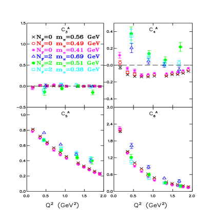
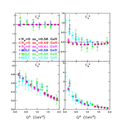
Figure 1: The axial form factors $C^{A}_{3}$, $C^{A}_{4}$, $C^{A}_{5}$ and $C^{A}_{6}$ as a function of $Q^{2}$. In all plots we show quenched results, denoted by $N_{f}=0$, at $\kappa=0.1554$ (crosses), at $\kappa=0.1558$ (open circles) and at $\kappa=0.1562$ (asterisks). The graphs on the left hand side also show unquenched Wilson results, denoted by $N_{f}=2$, at $\kappa=0.1575$ (triangles), $\kappa=1580$ (filled circles) and $\kappa=0.15825$ (open squares). The graphs on the right hand side also show results in the hybrid approach at $am_{l}=0.03$ (crosses), $am_{l}=0.02$ (filled diamonds) and $am_{l}=0.01$ (filled triangles).

In Fig. 1 we show our lattice results for the four axial form factors for quenched and unquenched Wilson fermions and in the hybrid approach. We observe that $C_{3}^{A}$ is consistent with zero and that unquenching effects are small for the dominant form factors, $C_{5}^{A}$ and $C_{6}^{A}$. The form factor $C_{4}^{A}$ shows an interesting behavior: The unquenched results for both dynamical Wilson and domain wall fermions show an increase at low momentum transfers. Such large deviations between quenched and full QCD results for these relatively heavy quark masses are unusual making this an interesting quantity to study effects of unquenching.

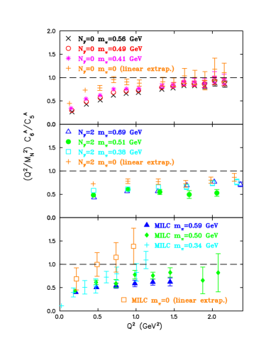
Figure 2: The ratio $\left(Q^{2}/M_{N}^{2}\right)C^{A}_{6}/C^{A}_{5}$ versus $Q^{2}$. Top: In the quenched theory, Middle: For dynamical Wilson fermions, Bottom: In the hybrid approach.

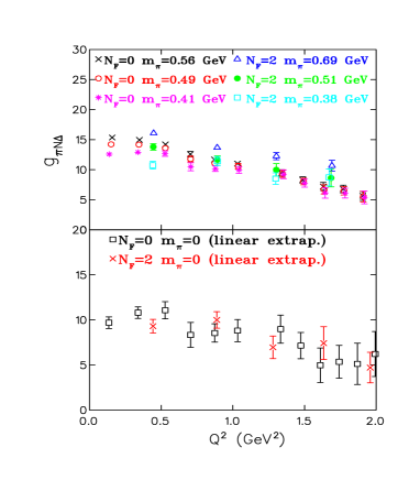
Figure 3: $g_{\pi N\Delta}$ as a function of $Q^{2}$ for quenched and dynamical Wilson fermions. Top: For our three-$\kappa$ values. Bottom: In the chiral limit.

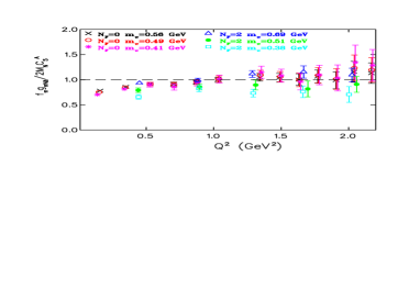
Figure 4: The ratio $f_{\pi}g_{\pi N\Delta}/\left(2M_{N}C^{A}_{5}\right)$ versus $Q^{2}$ for quenched and dynamical Wilson fermions.

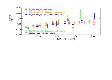
Figure 5: The ratio $C^{A}_{5}/C^{V}_{3}$ as a function of $Q^{2}$ for quenched QCD, for dynamical Wilson fermions and for the hybrid scheme.

In the chiral limit, axial current conservation leads to the relation $C_{6}^{A}(Q^{2})=M_{N}^{2}C_{5}^{A}(Q^{2})/Q^{2}$. In Fig. 3 we show the ratio $\left(Q^{2}/M_{N}^{2}\right)C_{6}^{A}(Q^{2})/C_{5}^{A}(Q^{2})$ for quenched and unquenched Wilson fermions, and in the hybrid scheme. In each case we show results for the available quark masses and in the chiral limit. The expected value in the chiral limit for this ratio is one. For finite quark mass the axial current is not conserved and for Wilson fermions chiral symmetry is broken so that deviations from one are expected. We observe that this ratio differs from unity at low $Q^{2}$ but approaches unity at higher values of $Q^{2}$. For the hybrid scheme the ratio is consistent with unity even at the lowest available $Q^{2}$, as expected for chiral fermions. That such chiral restoration is seen on the lattice even when using Wilson fermions demonstrates that lattice methodology correctly encodes continuum physics.

At finite pion mass partial conservation of axial current ($\partial_{\mu}A_{\mu}^{a}(x)=f_{\pi}m_{\pi}^{2}\pi^{a}(x)$) leads to the non-diagonal Goldberger-Treiman relation $C_{5}^{A}(Q^{2})=f_{\pi}g_{\pi N\Delta}(Q^{2})/2M_{N}$ where $g_{\pi N\Delta}(Q^{2})$ is determined from the matrix element of the pseudoscalar density

$$2m_{q}<\Delta^{+}(p^{\prime},s^{\prime})|\bar{\psi}\gamma_{5}\frac{\tau^{3}}{2}\psi|N(p,s)>=g_{\pi N\Delta}(Q^{2})\sqrt{\frac{2}{3}}\frac{q_{\sigma}}{2M_{N}}\frac{m_{\pi}^{2}f_{\pi}}{Q^{2}+m_{\pi}^{2}}\bar{u}_{\sigma}(p^{\prime},s^{\prime})u(p,s),$$ (4)

where $m_{q}$ is the renormalized quark mass. The pion decay constant, $f_{\pi}$, is determined from the two-point function $<O|A^{a}_{\mu}|\pi^{b}(p)>=ip_{\mu}\delta^{ab}f_{\pi}$, defined so that the continuum value is taken $f_{\pi}=93.2$ MeV. In order to relate the lattice pion matrix element to its physical value we need the pseudoscalar renormalization constant, $Z_{p}$. We take for quenched [13] and dynamical Wilson fermions [14] $Z_{p}(\mu^{2}a^{2}\sim 1)=0.5(1)$ computed using the RI-MOM method. This value may depend on the renormalization scale whereas it is not known for domain wall fermions. In Fig. 3 we show the result for $g_{\pi N\Delta}$ for Wilson fermions and the linear extrapolation in $m_{\pi}^{2}$ of these results to the chiral limit. We note that in the figure we only show statistical errors which do not include a 10% uncertainty in $Z_{p}$. Furthermore, we would like to stress that the determination of the quark mass $m_{q}$ using the axial Ward identity has corrections of order $a$. These corrections become more significant with decreasing quark mass. These can lead to large uncertainties in the determination of $g_{\pi N\Delta}$.

In Fig. 5 we show the ratio $f_{\pi}g_{\pi N\Delta}/\left(2M_{N}C_{5}^{A}\right)$ for Wilson fermions. As can be seen this ratio is almost $Q^{2}$ independent and as the quark mass decreases it becomes consistent with unity in agreement with the non-diagonal Goldberger-Treiman relation.

Under the assumptions that $C_{3}^{A}\sim 0$ and that $C_{4}^{A}$ is suppressed as compared to $C_{5}^{A}$, both of which are justified by the lattice results, the parity violation asymmetry can be shown to be proportional to the ratio $C_{5}^{A}/C_{3}^{V}$ [15]. The form factor $C_{3}^{V}$ can be obtained from the electromagnetic N to $\Delta$ transition. Using our lattice results for the dipole and electric quadrupole Sachs factors, ${\cal G}_{M1}$ and ${\cal G}_{E2}$ [11], $C_{3}^{V}$ is extracted from the relation $C_{3}^{V}=\frac{3}{2}\frac{M_{\Delta}(M_{N}+M_{\Delta})}{(M_{N}+M_{\Delta})^{2}+Q^{2}}\left({\cal G}_{M1}-{\cal G}_{E2}\right)$.

We show in Fig. 5 the ratio $C_{5}^{A}/C_{3}^{V}$, for pions of mass about 500 MeV. As can be seen unquenching effects are small and in order to assess the quark mass dependence we extrapolate our quenched results, which carry the smallest errors, to the chiral limit. We find only a small increase in this ratio as we tune the quark mass to zero, indicating a weak quark mass dependence. Therefore our lattice evaluation provides a prediction for the physical value of this ratio, which is the analog of the $g_{A}/g_{V}$. Our lattice results show that this ratio, and therefore to a first approximation the parity violating asymmetry, is non-zero at $Q^{2}=0$ and increases for $Q^{2}\stackrel{{\scriptstyle>}}{{\sim}}1.5$ GeV².

5 Conclusions

In summary we have provided a lattice calculation of the axial N to $\Delta$ transition form factors in the quenched approximation, using two degenerate dynamical Wilson fermions and within a hybrid approach where we use MILC configurations and domain wall fermions.

The main conclusions are: 1. $C_{3}^{A}$ is consistent with zero whereas $C_{4}^{A}$ is small but shows the largest sensitivity to unquenching effects. 2. The two dominant form factors are $C_{5}^{A}$ and $C_{6}^{A}$. These are related in the chiral limit by axial current conservation. The ratio $\left(Q^{2}/M_{N}^{2}\right)C_{6}^{A}/C_{5}^{A}$, which must be unity if chiral symmetry is unbroken, is shown to approach unity as the quark mass decreases. 3. For any quark mass the strong coupling $g_{\pi N\Delta}$ and the axial form factor $C_{5}^{A}$ show a similar $Q^{2}$ dependence with the non-diagonal Goldberger-Treiman relation being reproduced as the quark mass decreases. 4. The ratio of $C_{5}^{A}/C_{3}^{V}$ which determines to a good approximation the parity violating asymmetry is predicted to be non-zero at $Q^{2}=0$ and has a two-fold increase when $Q^{2}\sim 1.5$ GeV.

References

- [1] S. P. Wells, PAVI 2002, Mainz, Germany, June 5-8, 2002, and private communication.
- [2] B. Orth, Th. Lippert and K. Schilling, Phys. Rev. D72 (2005) 014503.
- [3] C. Urbach et. al, Comput. Phys. Commun. 174 (2006) 87.
- [4] K. Orginos, D. Tousaint and R. L. Sugar, Phys. Rev. D60 (1999) 054503.
- [5] R. G. Edwards, et al. (LPH Collaboration), Phys. Rev. Lett. 96 (2006) 052001.
- [6] C. Alexandrou et al., Nucl. Phys. B414 (1994) 815.
- [7] C. Alexandrou, G. Koutsou, J. W. Negele and A. Tsapalis, Phys. Rev. D74 (2006) 034508.
- [8] A. Hasenfratz and F. Knechtli, Phys. Rev. D64 (2001) 034504.
- [9] C. Alexandrou, Th. Leontiou, J.W. Negele and A.Tsapalis, hep-lat/0607030.
- [10] C. Aubin et al., Phys. Rev. D70 (2004) 094505.
- [11] C. Alexandrou et al., Phys. Rev. Lett. 94 (2005) 021601; PoSLat2005 (2006) 091.
- [12] C. Alexandrou, hep-lat/0609004.
- [13] V. Gimenez, L. Guitsit, F. Rapuano and M. Talevi, Nucl. Phys. B531 (1998) 429 .
- [14] D. Becirevic et al., Nucl. Phys. B734 (2006) 138.
- [15] N. C. Mukhopadhyay et al., Nucl. Phys. A633 (1998) 481.