The static quark potential for dynamical domain wall fermion simulations

Abstract:

We present preliminary results for the static quark potential computed on some of the DWF lattice configurations generated by the RBC-UKQCD collaborations. Most of these results were obtained using Wilson lines joining spatial planes fixed into the Coulomb gauge. We compare the results from this method with the earlier ones on $16^{3}\times 32$ lattices using Bresenham spatial paths with APE smeared link variables. Some preliminary results on $24^{3}\times 64$ lattices are also presented.

1 Introduction

The lattice scale is a very important quantity for lattice QCD, especially as we work toward more accurate results. Different from the methods of using hadronic masses and matrix elements to determine the lattice scale, the static quark potential provides an independent method. In this proceeding I will provide a status report on the RBC and UKQCD collaborations’ efforts to calculate the potential on $N_{f}=2+1$ domain wall fermion dynamical lattice configurations, and the preliminary results of the corresponding lattice spacing assuming $r_{0}=0.5fm$. The proceeding is organized as the following: first I start from the basic mathematical formulation of potential calculation, and introduce 2 different methods, Coulomb gauge method and Bresenham method. After explaining how to use the fitting methods to get the lattice spacing I will focus on the 3 specific ensembles of lattice configurations, and talk about the results and the underlying difficulties. Finally I conclude that the Coulomb method is much easier to implement and is reliable on large volume lattices.

2 The static quark potential and lattice scale

The static quark potential between infinitely heavy quark and anti-quark separated by $\vec{r}$ is calculated from the Wilson loop: $\left\langle W(\vec{r},t)\right\rangle=C(\vec{r})e^{-V(\vec{r})t}+(\mbox{"excited states"})$. Among the various ways to calculate the Wilson loop, we focus on 2 here: Bresenham method and Coulomb gauge method. While some smearing should be done on the spacial links in order to improve the signal/noise ratio, each method will implement the smearing in its own way.

The Bresenham method involves APE smearing for spatial links. While the on axis Wilson loops can be trivially calculated using the definition, for the off axis loops, one can implement the Bresenham algorithm [1] to approximate the diagonal path by the closest link path. This method was studied in detail in Ref. [2].

The Coulomb gauge method was first introduced in Ref. [3], The main idea is to gauge fix the lattices into the Coulomb gauge on each 3-dimensional plane orthogonal to the time direction, and then just compute the trace of the product of pairs of temporal links whose ends are fixed in Coulomb gauge.

In many respects, the two methods are quite different and have their own pros and cons. The Bresenham method uses APE smearing. By adjusting the smearing to maximize the overlap to the ground state it can safely eliminate most of the excited states contamination. On the other hand, the complexity involved in the various spacial paths makes the method hard to be parallelized when doing calculation numerically on parallel computers. For the Coulomb gauge method, it is open to question how much smearing the gauge fixing has done so the excited states contamination is not controlled. However, since the calculation after gauge fixing only needs the time direction links, its code is pretty easy to get parallelized. For example, when running on a 64-node QCDOC mother board the parallelized code takes about 4 minutes per configuration - about 40 times faster than the Bresenham code. We will see later that the finite size effects are much larger for the Coulomb than the Bresenham method. This will be discussed in the next section.

Here I carried out a study of Coulomb gauge method on the RBC-UKQCD 2+1 flavor domain wall fermion dynamical lattices with DBW2 and Iwasaki actions. The work was done on $16^{3}\times 32$ as well as $24^{3}\times 64$ lattices. The simulation lattices and corresponding results are listed in the Table 1. I will compare most of them to the results from Bresenham method when corresponding data are available and see how consistent these two methods are. As the Coulomb gauge method costs much less computational power we can have a lot more statistics easily. In addition to this, we can further improve the statistics by choosing the ”time” axis to lie along each of the four possible axes assuming the breaking of the $90^{o}$ rotation symmetry is negligible. We will confirm the symmetry breaking is small later in the results.

$\beta$	($m_{ud},m_{s}$)	# conf	$r_{0}/a$ (*)	$a^{-1}$[Gev](*)	$r_{0}/a$(2)	$a^{-1}$[Gev](2)
0.72	(0.01,0.04)	1000	3.962(30)	1.564(12)	3.947(38)	1.558(15)
0.80	(0.04,0.04)	200	5.014(38)	1.979(15)	4.763(44)	1.880(17)
$\beta$/Vol	($m_{ud},m_{s}$)	# conf	$r_{0}/a$ (1)	$a^{-1}$[Gev](1)	$r_{0}/a$(2)	$a^{-1}$[Gev](2)
	(0.01,0.04)	600	3.997(22)	1.577(9)	4.011(21)	1.583(8)
2.13	(0.02,0.04)	380	3.872(29)	1.528(11)	3.871(26)	1.528(10)
$16^{3}\times 32$	(0.03,0.04)	300	3.815(30)	1.506(12)	3.825(28)	1.510(11)
	-$m_{res}$	-	4.113(31)	1.623(12)	4.127(44)	1.629(17)
	(0.01,0.04)	200	4.071(18)	1.607(7)	4.056(14)	1.600(6)
2.13	(0.02,0.04)	200	3.946(12)	1.557(5)	3.947(11)	1.558(5)
$24^{3}\times 64$	(0.03,0.04)	200	3.869(19)	1.527(7)	3.876(11)	1.530(5)
	-$m_{res}$	-	4.191(31)	1.654(12)	4.163(24)	1.643(9)

Table 1: Preliminary results for the DWF dynamical Lattices analyzed in this work. The first 2 ensembles have DBW2 gauge action with volume $16^{3}\times 32\times 8$, and the $\beta=2.13$ ensembles have $Ls=16$ with Iwasaki gauge action. (1) denotes the exponential fit results, (2) is for the constant fit results and (*) is from the Bresenham. The chiral limit results are extrapolated by taking $m_{ud}=-m_{res}=-0.00308$.

The potential can be determined by fitting the approximate expression of the Wilson loop $\left\langle W(\vec{r},t)\right\rangle=C(\vec{r})e^{-V(\vec{r})t}$. one can either fit this using (1) “exponential fit”: fit the Wilson loop as an exponential function of $t$ to extract $V(\vec{r})$ or (2) “constant fit”: fit the quantity $V(\vec{r},t)=\mbox{ln}[\left\langle W(\vec{r},t)\right\rangle/\left\langle W(\vec{r},t+1)\right\rangle]$ to a constant in $t$. The double exponential fit is also an option if we take into account the lowest excited states contamination, but it is very unstable. All the analysis in this proceeding for the potential are either constant fit or exponential fit.

Having determined the potential, one can calculate the lattice scale by fitting the potential to the form: $V(\vec{r})=V_{0}-\alpha/|\vec{r}|+\sigma|\vec{r}|$. Then the Sommer scale $r_{0}/a=\sqrt{(1.65-\alpha)/\sigma}$ is determined in lattice units. The lattice scale can be obtained by assuming the physical value of $r_{0}$ to be 0.5 fm.

3 Finite size effect

The Coulomb gauge method suffers from the enhanced finite size effect. Quark states have images on the neighbor lattices due to the periodic boundary condition. As the Wilson loop calculation doesn’t involve spacial links connecting the quark and anti-quark states, the images will have considerable contribution to the Wilson loops in the Coulomb method. In contrast, the Bresenham method prevents the images in the wall from having much effect with explicit Wilson lines connecting specific pairs of Wilson lines in the time-direction.

4 Results

In this section, the Coulomb results on the potential and $r_{0}$ will be compared to the Bresenham ones on all the 3 ensembles - $\beta=0.72$, $\beta=0.80$ and $\beta=2.13$(Tab. 1). Since we incorporated into the analysis our technique to increase the statistics by 4 with ”time” direction choices, we investigate how big is the rotational symmetry breaking. Fig. 2 is an example of the direction dependence of the potential on $\beta=2.13$, $16^{3}\times 32$, $m_{ud}=0.01$ lattices. The figure indicates the symmetry breaking is negligible. All the results for the Coulomb method are based on averaging potentials from 4 directions for each configuration. The Bresenham results are quoted from Ref. [2] and are calculated with only one “time” axis. All errors are statistical only.

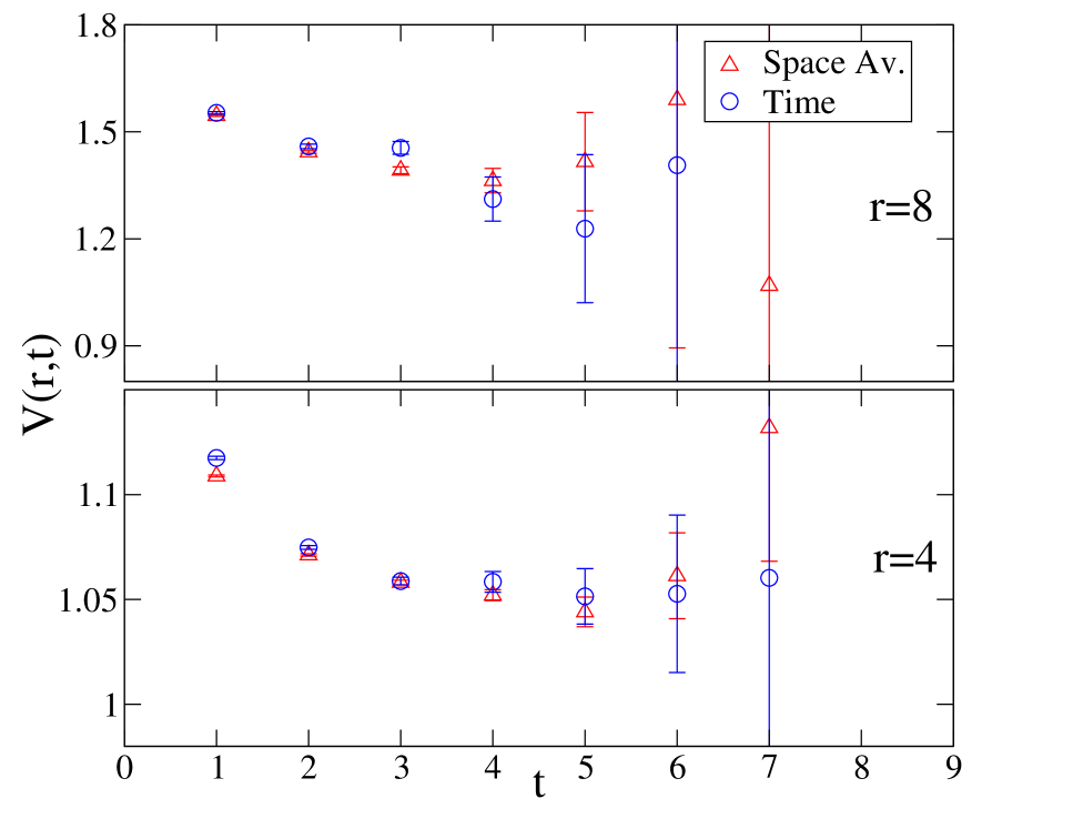
Figure 1: The direction dependence of the potential for $\beta=2.13$, $16^{3}\times 32$: the spacial results averaged (triangle) and time results (circle).

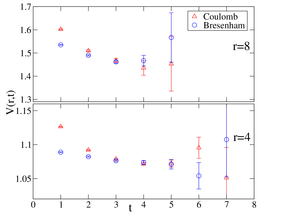
Figure 2: The time dependence of potential at fixed $r$’s for Coulomb (triangle) and Bresenham (circle) on $\beta=0.72$ ensemble.

4.1 $\beta=0.72$ ensemble

As we use the constant fit, the potential obtained has dependence on the time. And as the time increases, the excited states contamination will decrease exponentially. Fig. 2 shows the $t$ dependence of the potential at various $r$’s for the Bresenham and Coulomb methods. The results presented here are based on 1000 configurations for the Coulomb method and 900 configurations for the Bresenham method. Both methods show good plateaus and the potential values are consistent within the error bar when they reach the plateau.

For $r_{0}$, we fit the potential as a function of $r$ at each time slice. In order to get a sense of how different is Coulomb from Bresenham, we choose the $r$ fitting range the same as in Ref. [2]: $\sqrt{3}$ to 8, the value quoted here is from $t=5$ only. The comparison is given in Fig. 4, which shows that (1) Both methods have good plateaus indicating that the excited states contamination is negligible; (2) $r_{0}$ values agree very well within error bars; (3) The errors are small(¡1%).

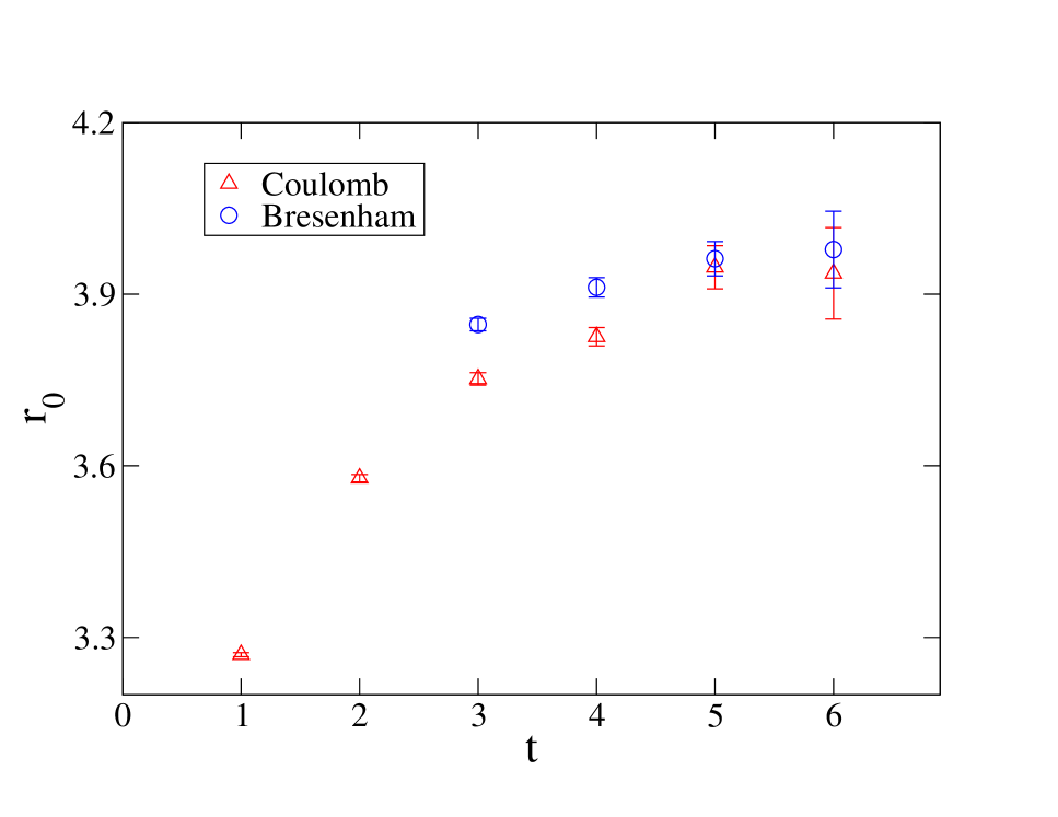
Figure 3: The time dependence of $r_{0}$ for Coulomb (triangle) and Bresenham (circle) on $\beta=0.72$ ensemble.

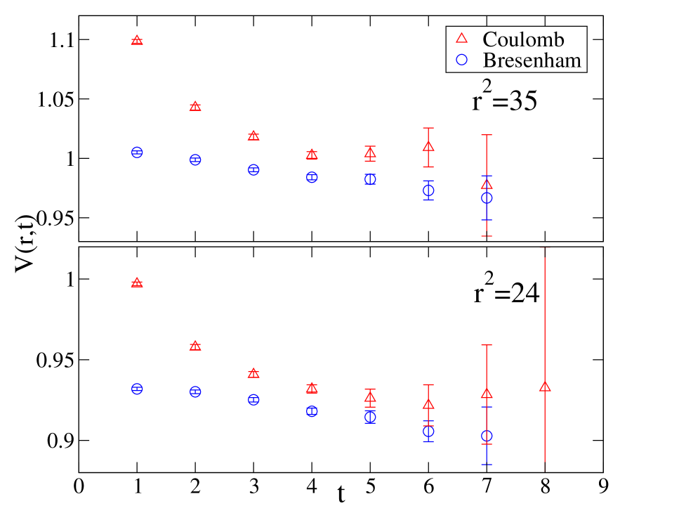
Figure 4: The time dependence of potential at some off-axis $r$’s for Coulomb (triangle) and Bresenham (circle) on $\beta=0.80$ ensemble.

4.2 $\beta=0.80$ ensemble

In this case, the finite size effect seems to have a large impact. The results for both methods are based on the same 200 configurations. To see a similar plot as in Fig. 2 for $\beta=0.72$, we plot several off-axis $r$’s in Fig. 4 as these manifest the potential differences. The $r$ dependence of the potential is given in Fig.  6 for $t=5$.

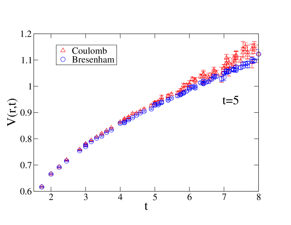
Figure 5: The $r$ dependence of potential for Coulomb (triangle) and Bresenham (circle) on $\beta=0.80$ ensemble.

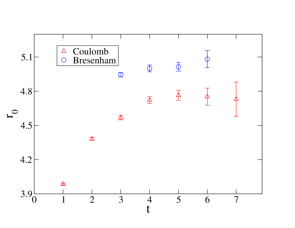
Figure 6: The time dependence of $r_{0}$ for Coulomb (triangle) and Bresenham (circle) on $\beta=0.80$ ensemble.

The fitted $r_{0}$ values at different times are plotted in Fig. 6. We get $r_{0}=4.763(44)$ for the Coulomb method and $r_{0}=5.014(38)$ for the Bresenham method, both from $t=5$ only. There is a  4-5% discrepancy. By looking at the potential [Fig. 6], it seems consistent that the finite size effect has much more impact on larger $r$. And if we shrink the fitting range to smaller $r$’s, one would expect the potential for the two methods to become more and more consistent, thus the $r_{0}$ for the Coulomb method will also increase to match the Bresenham. Although the $r_{0}$ and potential have large discrepancy for this ensemble, it doesn’t mean that the Coulomb method is wrong and unreliable. To solve this problem, we can either use a large volume lattice, or shrink the fitting range.

4.3 $\beta=2.13$ ensemble

Here we have both $16^{3}\times 32$ and $24^{3}\times 64$ ensembles, and for each ensemble 3 different sea quark masses are available so we can do chiral extrapolation and set the lattice scale. The comparison between $16^{3}\times 32$ and $24^{3}\times 64$ are plotted for $m_{ud}=0.01$ case. From the potential plot [Fig. 8, 8] we can see that the $24^{3}\times 64$ results are a bit lower at large r, which is consistent with the proposed image problem. But since the $Ls$ is different from $\beta=0.80$, there might be contamination from other effects here. For the exponential fit, time range is from 4 to 6. The constant fit results for $r_{0}$ are error weighted from t=4 to 6.

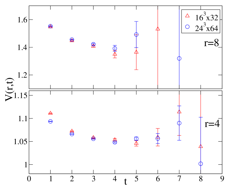
Figure 7: The $r$ dependence of potential for Coulomb method on $\beta=2.13$, $m_{ud}=0.01$, $16^{3}\times 32$ and $24^{3}\times 64$ lattices.

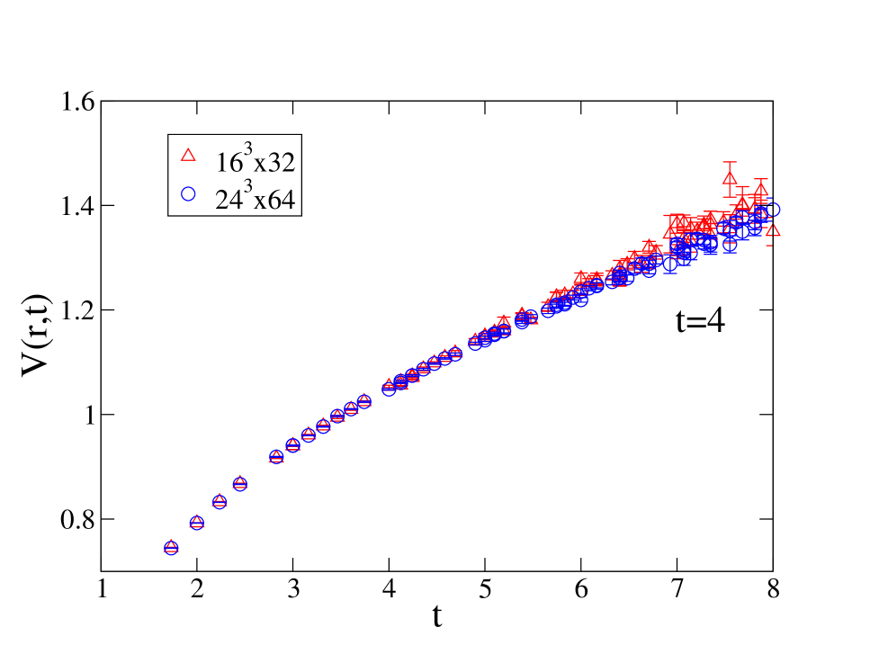
Figure 8: The potential comparison between $16^{3}\times 32$ and $24^{3}\times 64$ lattices for $\beta=2.13$ ensemble.

The $r_{0}$ results from 3 different $m_{ud}$ are shown in Fig. 9. From the results of 2 volumes, unitary chiral extrapolation to the chiral limit give us the $r_{0}$ and the lattice scale $a^{-1}$, see Fig. 11. The $r_{0}$ values from $16^{3}\times 32$ are a bit lower. This is consistent with our observation on $\beta=0.80$.

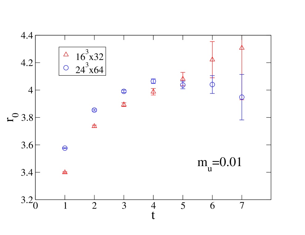
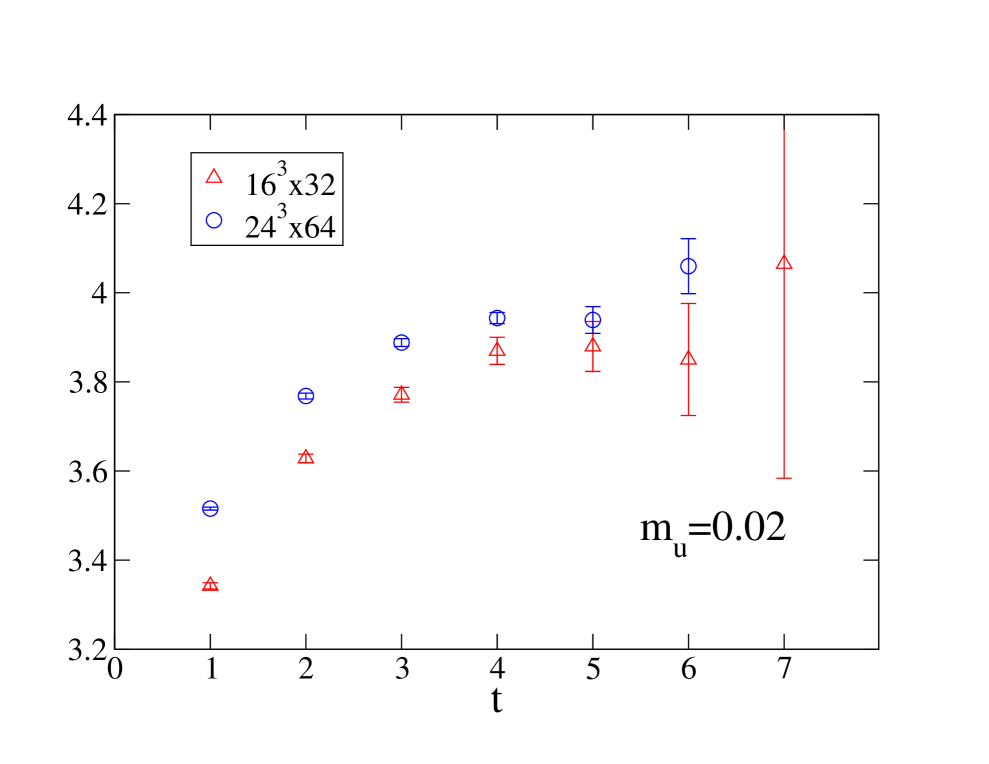
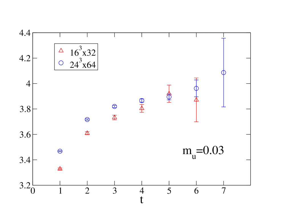
Figure 9: The $r_{0}$ comparison between $16^{3}\times 32$ and $24^{3}\times 64$ lattices on $\beta=2.13$ ensemble.

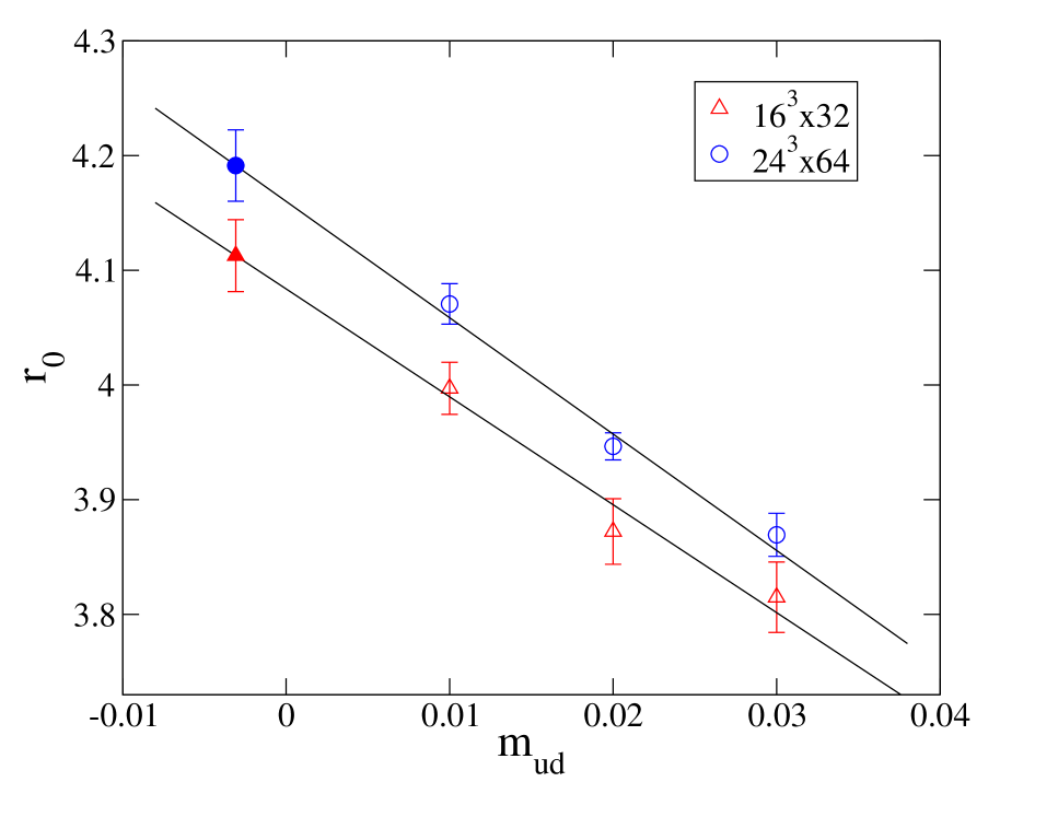
Figure 10: Unitary chiral extrapolations for $r_{0}$ for $\beta=2.13$ ensemble on $16^{3}\times 32$ and $24^{3}\times 64$ lattices. Data are from exponential fit only.

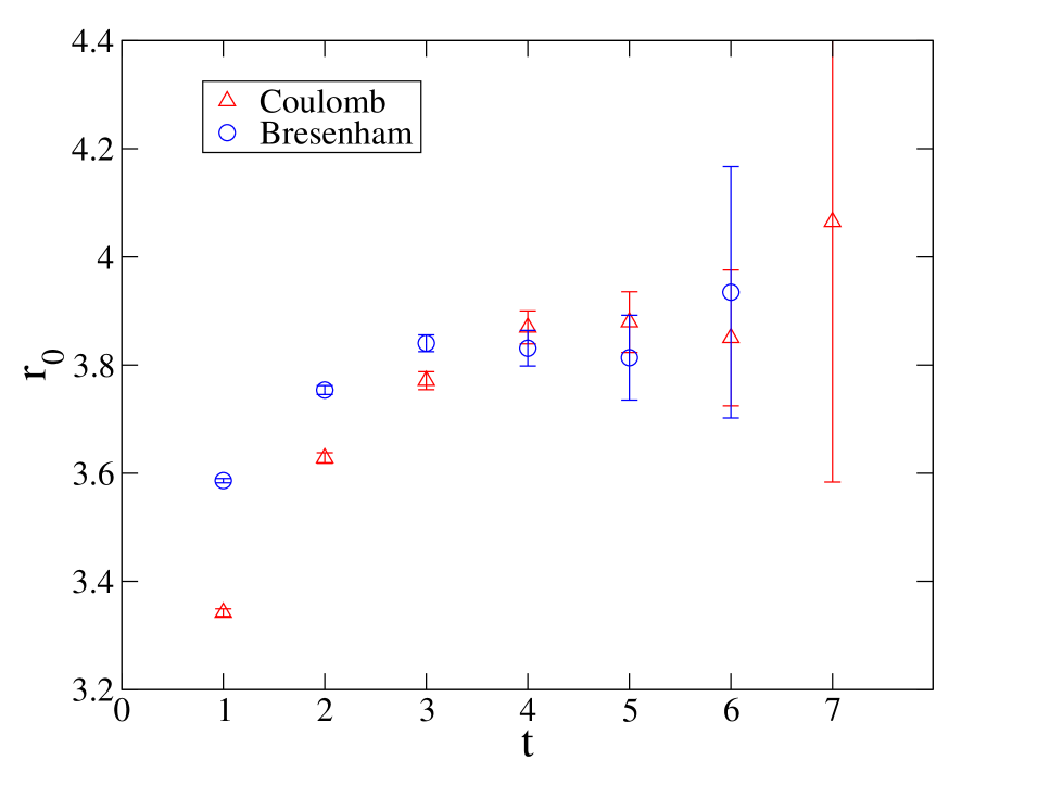
Figure 11: The Coulomb (triangle) and Bresenham (circle) results for $r_{0}$, on the $\beta=2.13$, $16^{3}\times 32$, $m_{ud}=0.02$ lattice.

Although the Bresenham results for the $\beta=2.13$ ensembles are not available in Ref [2], I ran a parallelized QCDOC Bresenham code written by Takashi Umeda without tuning the APE smearing steps (fixed to 25) and produced some preliminary results for $\beta=2.13$, $16^{3}\times 32$, $m_{ud}=0.02$ case. As shown in Fig. 11, the plateaus are good and the $r_{0}$ values are consistent. This indicates that the potential and lattice scale set by the Coulomb method is quite reliable.

5 Summary and Conclusion

We compare the Coulomb gauge method and the Bresenham method in different cases, and draw the conclusion that the Coulomb method is much easier to implement but is more susceptible to finite size effects when the physical volume is small. We proposed the interaction with images as a possible explanation for the finite size effects. Although we haven’t found a good way to eliminate the effects, a larger volume and a smaller fitting range for $r_{0}$ are candidates to make them negligible. The results on the $\beta=2.13$, $16^{3}\times 32$, $m_{ud}=0.02$ lattice for the Bresenham and Coulomb method are consistent. It indicates that the finite size effect doesn’t contribute much here so the chiral extrapolated $r_{0}$ and lattice scale set by this method should be reliable. And so does the $24^{3}\times 64$ case, in which the lattice has a much larger volume.

References

- [1] B. Bolder et al., A High Precision Study of the Potential from Wilson Loops in the Regime of String Breaking, Phys. Rev. D63 (2001) 074504, [hep-lat/0005018].
- [2] K. Hashimoto and T. Izubuchi, The static quark potential in 2+1 flavour Domain Wall QCD from QCDOC, PoS LAT2005 (2005) 093, [hep-lat/0510079].
- [3] C. Bernard et al., Static quark potential in three flavor QCD, Phys. Rev. D62 (2000) 034503, [hep-lat/0002028].