Pure SU(3) lattice gauge theory
using operators and states

Abstract

We study pure SU(3) gauge theory on a large lattice, using Schrödinger’s equation. Our approximate solution uses a basis of roughly 1000 states. Gauge invariance is recovered when the color content of the ground state is extrapolated to zero. We are able to identify the gauge invariant excitations that remain when the extrapolation is performed. In the weak coupling limit, we obtain promising results when we compare the excitation energies (masses) to known exact results, which we derive. We discuss the application of our nonperturbative method in the regime where glueballs are present.

I Introduction.

Pure SU(3) gauge theory on the lattice can be formulated in Hamiltonian form. Matrix elements of the Hamiltonian using any finite orthonormal basis can be used to form a Hamiltonian matrix, and the eigenvalues of this matrix, ordered in increasing energy, are each an upper limit to the corresponding eigenvalue of the original Hamiltonian.A If the basis is provided with parameters, these can be used to lower the approximate energies closer to their true values.

Variational calculations run into problems unless the basis states are carefully chosen. This is particularly true when many degrees of freedom (DF) are involved. The most serious problem is that the eigenvalues of the matrix may be useless because they lie far above the eigenvalues of the Hamiltonian and do not accurately portray the physical implications of the Hamiltonian, quantitatively or even qualitatively. Another problem associated with many DF is that the basis size can become unmanageable. If we work on a $L\times L\times L$ spatial lattice, there are $24L^{3}$ degrees of freedom. (There are 3 links emerging from each site on the lattice, and 8 colors per link.) When we introduce two states for each DF, as we will, we have a basis of $2^{24L^{3}}$ states. Further cuts must be made. As we do this, we also want to build symmetries of the Hamiltonian into the basis so that quantum numbers can be assigned to the eigenvalues of the matrix. The foundation of a variational calculation is therefore the crafting of a well-chosen basis.

The main purpose of this paper is to construct a basis for pure SU(3) lattice gauge theory and demonstrate that it is well-chosen. In this Introduction we outline the issues that must be faced in the construction process, and how we cope with them. In following sections we compare results obtained with our basis to known results, thus testing the adequacy of the basis. This comparison can be made only in a limiting case, but that case imposes significant tests. The methods we use can be applied away from the limit to the “physical” case, where the lattice is inhabited by glueballs. We outline how to do this at the end of the paper.

The approach we take in this paper is clearly an approximation. On the other hand, the customary evaluation of the path integral by Monte Carlo sampling can, in principle, be arbitrarily accurate as more computing resources are devoted to the project. But that project has been ongoing for 30 years, using the most advanced computing facilities in the world. The payoff to our approach is that the computer resources required are very modest.

I.1 The Hamiltonian

We begin with a description of the elements required to write the Hamiltonian for pure SU(3) local gauge theory on a three dimensional lattice. We label links on our lattice by the pair $({\bf s},m)$, where $\bf s$ is the site from which a link departs, with $0\leq s_{x},s_{y},s_{z}\leq L\equiv 0$, and the lattice is an $L\times L\times L$ cube. $m=x$, $y$ or $z$ is the direction of the link. The variables assigned to a link degree of freedom specify a point on the SU(3) manifold, a compact manifold of eight dimensions labelled by $a=1,\dots,8$, the color index. In the Hamiltonian we use the fundamental representation matrix $U_{{\bf s},m}$, which depends on the point on SU(3) for link $({\bf s},m)$. We also use the operators ${\cal J}_{L,a}({\bf s},m)$ with $a=1,\dots,8$. The action of ${\cal J}_{L,a}$ on a representation of SU(3) is to left-multiply it by the $a$th generator matrix for that representatrion. Similarly, ${\cal J}_{R,a}$ acts to right-multiply. ${\cal J}^{2}=\sum{\cal J}^{2}_{L,a}=\sum{\cal J}^{2}_{R,a}$ multiplies by the quadratic Casimir operator for SU(3). The Hamiltonian is then:

$$H_{A} = \sum_{\bf s}H({\bf s}),$$

$$H({\bf s}) = \frac{g^{2}}{2}\sum_{m}{\cal J}^{2}({\bf s,m})-\frac{1}{g^{2}}$$ (1)

$$\times\sum_{m<n}\left[{\rm Tr}\left(U_{{\bf s},m}U_{{\bf s+\hat{m}},n}U^{\dagger}_{{\bf s+\hat{n}},m}U^{\dagger}_{{\bf s},n}\right)+{\rm H.c.}-6\right].$$

$H_{A}$ is the Kogut-Susskind Hamiltonian.D It commutes with the generators of local gauge transformations at site ${\bf s}$:

$$Q_{a}({\bf s}) = -{\cal J}_{L,a}({\bf s},x)-{\cal J}_{L,a}({\bf s},y)-{\cal J}_{L,a}({\bf s},z)$$ (2)

$$+{\cal J}_{R,a}({\bf s-\hat{x}},x)+{\cal J}_{R,a}({\bf s-\hat{y}},y)$$

$$+{\cal J}_{R,a}({\bf s-\hat{z}},z).$$

The Hamiltonian formulation of lattice gauge theory has been used for a number of studies, mostly based on loop expansions that differ from the approach we take here. For a recent review, see J .

I.2 States for Each Link.

The first step in building a basis is to choose states on the SU(3) manifold for each link. To make the choice, we need to know where on the manifold the eigenfunctions of $H_{A}$ have support (are large), and this depends on the coupling $g$. We begin with small $g$. It is convenient to use the parametrization for the fundamental representation matrix

$$U=\exp(ig\lambda_{a}R_{a}/2)$$ (3)

where $\lambda_{a}$ is a Gell-Mann matrix.B We next develop ascending power series in $g$ for the elements in the Hamiltonian

$${\cal J}_{L,a} = \frac{1}{ig}\frac{\partial}{\partial R_{a}}+\frac{i}{2}f_{abc}R_{b}\frac{\partial}{\partial R_{c}}+\cdots,$$

$${\cal J}_{R,a} = \frac{1}{ig}\frac{\partial}{\partial R_{a}}-\frac{i}{2}f_{abc}R_{b}\frac{\partial}{\partial R_{c}}+\cdots,$$ (4)

$$U = 1+\frac{ig}{2}(\lambda_{a}R_{a})-\frac{g^{2}}{8}(\lambda_{a}R_{a})^{2}\cdots.$$

To study support, we examine a “lattice” consisting of one link. To lowest order in $g$, the Hamiltonian is

$$H^{\prime}=\frac{g^{2}}{2}{\cal J}^{2}-\frac{1}{g^{2}}\left[2{\rm Tr}U-6\right]=-\frac{1}{2}\frac{\partial^{2}}{\partial{\bf R}^{2}}+\frac{{\bf R}^{2}}{2}.$$ (5)

If we treat $\bf R$ as an eight dimensional Euclidean vector, the ground state of $H^{\prime}$ is

$$\psi=\exp(-{\bf R}^{2}/2).$$ (6)

The Euclidean approximation is justified when $g$ is small because then the group parameters $\alpha_{a}=gR_{a}$ are small where the wave function is large, and the fact that SU(3) is not Euclidean can be ignored. At weak coupling, therefore, wave functions have support only near the group origin. As $g$ grows, the region on the manifold where the wave function is large expands. At large $g$ we know from strong coupling expansions that wave functions have support everywhere on the manifoldD . Therefore, we seek Gaussian-like states on the manifold, centered on the origin, with width that can be tuned as a variational parameter.

Gaussian-like states on the group are generated by the kernel of the heat equationC .

$$\frac{d\phi}{dt}={\cal J}^{2}\phi.$$ (7)

The weak coupling, Euclidean approximation demonstates that the kernel is Gaussian:

$$\frac{d\phi}{dt}=\frac{1}{g^{2}}\nabla^{2}\phi,\qquad\langle{\bf R_{1}}|e^{t\nabla^{2}/g^{2}}|{\bf R_{2}}\rangle=\frac{e^{-g^{2}({\bf R_{1}-R_{2}})^{2}/4t}}{(4\pi t/g^{2})^{4}}.$$ (8)

We will use the scaled width variable $\tau=t/g^{2}$. Comparing Eqs. (6) and (8), for one link at weak coupling $\tau=1/2$. This is the order of magnitude for $\tau$ that we will find for a large lattice at weak coupling.

The heat kernel on SU(3) isE

$$\psi_{\alpha_{1}}(\alpha) = \langle\{\alpha\}|e^{-t{\cal J}^{2}}|\{\alpha_{1}\}\rangle$$

$$= \sum_{p,q}d(p,q)e^{-t\lambda(p,q)}\chi^{(p,q)}(\{\alpha\}\{\alpha_{1}\}^{-1}),$$

where $\{\alpha\},\ \{\alpha_{1}\}$ are group parameters, $\chi^{(p,q)}$ is the character, $d(p,q)$ is the dimension of representation $(p,q)$, and $\lambda(p,q)$ is the Casimir eigenvalue.E ; F Note that when $t$ is small (narrow Gaussian), many representations contribute. This mirrors the situation in Euclidean space, where many harmonics are required to build up a narrow Gaussian.

In Eucliean space, Gaussians can be extended to a complete set of basis states by multiplication by polynomials or by differentiation, and the same can be done on SU(3). The simplest of these states are

$$\phi=\psi_{\alpha 1}(\alpha)|_{\alpha_{1}=0},$$ (10)

$$\phi_{a}={\cal J}_{La}(\alpha_{1})\psi_{\alpha_{1}}(\alpha)|_{\alpha_{1}=0}.$$

The orthogonality properties of these states areE

$$\langle\phi|\phi\rangle = S_{1};\quad\langle\phi_{a}|\phi\rangle=0;\quad\langle\phi_{a}|\phi_{b}\rangle=\delta_{ab}S_{2};$$

$$S_{1} = \sum_{p,q}d^{2}(p,q)e^{-2t\lambda(p,q)};$$ (11)

$$S_{2} = \frac{1}{8}\sum_{p,q}d^{2}(p,q)\lambda(p,q)e^{-2t\lambda(p,q)}.$$

Matrix elements of the operators in Eq. (I.1) among states $\phi$ and $\phi_{a}$ are computed in Ref. E . The dynamics of SU(3) is invoked through the use of these matrix elements.

On each link, we allow single excitations to occur in each of the eight colors. We exclude states that are multiply excited in the same color direction. Since each of the eight color directions on a link can be unexcited ($\phi$-like) or singly excited ($\phi_{a}$-like), our basis has $2^{8}=256$ states per link. An important topic of the paper will be to test the adequacy of limiting the basis to 256 states on each link in this way.

States in which two color directions on a link are excited, designated $\phi_{ab}$, are studied in Ref. E , but states in which $3,\dots,8$ directions are excited have not been studied. Extending the number of color directions excited on a link in the explicit manner of Ref. E is laborious and will not be attempted in this paper. The process is also ambiguous because the operator ${\cal J}_{La}$ used in the definition of $\phi_{a}$ and $\phi_{ab}$ can be replaced by others, like ${\cal J}_{Ra}$. Instead, in this paper we introduce states with “multi-color” excitations on a link, and matrix elements involving these states, in a straighforward way we describe in the next subsection.

I.3 States on the Lattice

The lattice basis constructed by putting each link in one of the 256 states we have introduced has $(256)^{3L^{3}}=2^{24L^{3}}$ elements, which is far too many to handle. In addition, local degrees of freedom constitute an awkward basis for describing phenomena that range over many links. Continuum field theory instructs us how to depart from local degrees of freedom by recasting the theory in momentum space. We adopt that method in this paper.

We introduce operators $A_{a}({\bf s},m)$. These are bosonic, satisfying the usual bosonic commutation rules. The ground state $|0\rangle$ corresponds to the normalized state $|\phi\rangle/\sqrt{S_{1}}$ on a link, and $-iA_{a}^{\dagger}|0\rangle$ corresponds to the state $|\phi_{a}\rangle/\sqrt{S_{2}}$ on the link. At this point we can describe how we represent a normalized state in which two distinct colors are excited on the same link; it is $(-iA_{a}^{\dagger})(-iA_{b}^{\dagger}|0\rangle$, where $a\neq b$.

We now follow field theory and introduce nonlocal states by passing to momentum space, introducing the bosonic operators

$$B_{a}({\bf k},m)=\frac{1}{L^{3/2}}\sum_{\bf s}e^{-2\pi i{\bf k\cdot}({\bf s+\hat{m}}/2)/L}A_{a}({\bf s},m).$$ (12)

I.4 The Basis Generator G

We return to the requirement that the state on each link be required to be in one of 256 states. Applications of operators $(-iA_{a}^{\dagger})^{k}$ with $k\geq 2$ produce states beyond the ones we’ve introduced. We refer to such states as “overexcited”. Overexcited states will appear unless we suppress them. First we introduce an operator that measures the excitation of the color/link degrees of freedom. It is

$$N=\sum_{{\bf s},m,a}A_{a}^{\dagger}({\bf s},m)A_{a}({\bf s},m),$$ (13)

A color/link degree of freedom in the $k$-th bosonic state is an eigenfunction of $N$ with eigenvalue $k$. Our method of minimizing the contribution of overexcited states to our basis is to control the expectation value of $N$ in our basis states.

With the introduction of $N$, we can begin to construct the basis. First we write $H_{A}$ in terms of our bosonic operators. Coefficients are chosen so that matrix elements on the basis of the two states for each color/link agree with matrix elements derived in Ref. E . Next we decompose $H_{A}$ into a term $H_{A,0}$, quadratic in $A$ and $A{{}^{\dagger}}$ and a remainder:

$$H_{A}=H_{A,0}+H_{A,1}$$ (14)

Equipped with this decomposition, we construct a generator operator $G$, whose low-lying eigenstates will compose our basis. The first expression for $G$ is

$$G_{A}=H_{A,0}+\xi N.$$ (15)

By limiting $G_{A}$ to quadratic terms, it becomes an operator that can be diagonalized. Its eigenstates can be constructed, leading to an explicit basis. We take $\xi$ to be a positive parameter, so the term $\xi N$ in $G_{A}$ reduces the contribution of overexcited states to the low energy spectrum of $G_{A}$, where the states in our basis are found. By changing $\xi$, we can adjust $\langle N\rangle$ for the eigenstates of $G_{A}$. Define $N_{ave}$ to be the expectation of $N$ per color/link DF in the ground state of $G_{A}$: $N_{ave}=\langle 0|N|0\rangle/(24L^{3})$. Most of our simulations will be carried out with $N_{ave}=1/2$. This small value suggests that the probability of finding a color/link to be overexcited is small, and it is. We will present a formula giving the probability that a color/link is in any overexcited state, and the typical result (when $N_{ave}=1/2$) is about 1/8. Therefore, overexcited states contribute to results computed in our basis, but not much. We have some ability to check on the influence of overexcited states by changing $\xi$ and hence $N_{ave}$. We do not want to make $N_{ave}$ too small, however, because we do not want to suppress the 256 states we allow for each link. Another method of excluding overexcited states would be to map pure SU(3) onto a spin model, with each color/link being in either a “spin up” or “spin down” state. This would eliminate overexcited states altogether, but it would deny us the methods of field theory, particularly the simple introduction of nonlocal degrees of freedom by transforming to momentum space.

To summarize our procedure, we have adopted a bosonic formalism. This allows us to pass to momentum space and construct a basis that is nonlocal. The price we pay is that there are contributions from overexcited bosonic states that are unwanted. By taking our basis states to be eigenstates of the generator $G_{A}$, we can use the parameter $\xi$ to minimize and assess the effects of the overexcited states.

I.5 Gauge Invariance

We seek states having $Q_{a}({\bf s})|\psi\rangle=0$. There are three options for excluding non-gauge invariant states. One is to rewrite the theory in terms of gauge invariant DF only. Unfortunately, the resulting Hamiltonians are nonlocal and are not manifestly under rotations of the cubic latticeG ; H . They are unsuited for approximation schemes. The second option is to use Hamiltonian (I.1) but allow only gauge invariant states in the basis. This is done when loop expansions are employed.J However, sound arguments have led us adopt the eigenstates of $G_{A}$ as basis states, and these states are not gauge invariant.

The third option is to compute with a nonzero expectation value, per site, of the group quadratic Casimir operator: $Q_{ave}^{2}=\langle 0|Q^{2}|0\rangle/L^{3}$. Here $|0\rangle$ is the ground state of $G_{A}$, and

$$Q^{2}=\sum_{{\bf s},a}Q_{a}({\bf s})^{2}.$$ (16)

This is the option we adopt. We will calculate results for several values of $Q_{ave}^{2}$ and extrapolate to the limit $Q_{ave}^{2}=0$ at the end. This was done successfully for the ground state in Ref. A , and we use the same method here. Note that $Q_{a}({\bf s})^{2}$ is a positive operator, so when $Q_{ave}^{2}=0$, gauge invariance is imposed at every site on the lattice.

Once we include gauge non invariant states in our basis, we want to control their number. This can be accomplished by adding a term to $G$ that raises the eigenvalue of such states. To do this, we decompose $Q^{2}$ into quadratic and higher terms, just as we did for $H_{A}$

$$Q^{2}=Q_{0}^{2}+Q_{1}^{2}.$$ (17)

We add term proportional to $Q_{0}^{2}$ to our generator, which we call $G_{B}$ after the modification.

$$G_{B}=G_{A}+\eta g^{2}Q_{0}^{2}=H_{A,0}+\xi N+\eta g^{2}Q_{0}^{2}.$$ (18)

The factor $g^{2}$ is included because $g^{2}Q^{2}_{ave}$ is finite as $g\rightarrow 0$.

Finally we introduce $H_{B}$, the Hamiltonian we use in the rest of this paper.

$$H_{B}=H_{A}+\eta g^{2}Q^{2}.$$ (19)

$H_{A}$ and $H_{B}$ have the same set of physical, gauge invariant eigenstates. However, the non-gauge invariant eigenstates of $H_{B}$ are raised in energy by the positive operator $\eta g^{2}Q^{2}$. By varying $\eta$ we can control the number of gauge non invariant states in the low energy spectrum.

Our basis states are the low-lying eigenstates of generator $G_{B}$. To diagonalize $G_{B}$ we must remove operators of the form $B^{\dagger}B^{\dagger}$ and $BB$. This is accomplished by means of the Bogoliubov transformation to new bosonic operators $E$:

$$B_{a}({\bf k},m)=$$

$$\cosh\theta({\bf k})E_{a}({\bf k},m)-\sinh\theta({\bf k})E^{\dagger}_{a}({\bf L-k},m),$$

with $\theta({\bf k})=\theta({\bf L-k})$ and ${\bf L}=(L,L,L)$. (Directional indices for $\theta$ will be introduced later, after we transform to the polarization basis.) We use the vacuum state of $G_{B}$ after the Bogoliubov transformation to determine the expectation values $N_{ave}$ and $Q_{ave}^{2}$. These parameters are set primarily by choice of $\xi$ and $\tau$. $\eta$ is used to set the number of non gauge invariant states in the low energy spectrum of $G_{B}$.

I.6 Group Theory, Degeneracy and Spin

Hamiltonian (I.1) is invariant under the group of rotations of the cubic lattice. Associated with this symmetry is degeneracy; states belonging to different rows of the same irreducible representation of the group are degenerate. Such degeneracy complicates computer work. It can be reduced by forming linear combinations of our basis states that belong to the same row of an irreducible representation of the group:

$$|\psi\rangle=\sum_{R}{\cal D}^{(J)*}_{\mu\nu}(R)U(R)|a\rangle,$$ (21)

where ${\cal D}^{(J)}$ is an irreducible representation of the group, and $U(R)|a\rangle$ is the image of $|a\rangle$ under a rotation of the cube.

The group of rotations of the cube has 24 elementsI . It has five irreducible representations (because there are five classes), which we label by their dimensions: $1_{A}$, $1_{B}$, $2$, $3_{A}$ and $3_{B}$. (The sum of the squares of these dimensions is the order of the group, implying that Eq. (21) provides 24 states for each $|a\rangle$.)

An additional reason to take account of the symmetry group is that we wish to identify the spins of the states we find. Since our lattice breaks the O(3) symmetry of continuum field theory, this identification is not obvious. Note, however that each of the 24 rotations of the cube corresponds to an element of O(3). The identity element corresponds to a rotation by $0^{\circ}$, and each of the other elements corresponds to a rotation by $90^{\circ}$, $120^{\circ}$ or a multiple of these about an axis through the center of the cube. It follows that every irreducible representation of O(3) generates a representation of the group of the cube, which is generally reducible. The first few Clebsch-Gordon series giving the content of O(3)-induced representations are

$$({\rm spin0}) \longrightarrow 1_{A},$$

$$({\rm spin1}) \longrightarrow 3_{A},$$ (22)

$$({\rm spin2}) \longrightarrow 2\oplus 3_{B},$$

$$({\rm spin3}) \longrightarrow 1_{B}\oplus 3_{A}\oplus 3_{B}.$$

In these four cases, a representation of the group of the cube is identified with a spin. However, an eigenstate belonging to the $2$ representation of the cube can be associated with spin 2 only if there is an eigenstate belonging to the $3_{B}$ of nearly the same energy. If this is not the case, it may not be possible to identify the $2$ eigenstate with a continuum state.

In this paper we will study spin 0 states. ${\cal D}(R)=1$ for this case, and

$$|\psi\rangle=A\sum_{R}U(R)|a\rangle$$ (23)

II Weak Coupling

We need a known reference theory which we can use to evaluate the adequacy of the approximations laid out in Sec. I. For this pupose we use the weak coupling limit of the theory. This is the limit in which the correlation length has grown beyond the lattice length $L$. This regime is reached for couplings $g$ below those in the scaling region in which glueballs are dynamically contained within the lattice. The weak coupling limit is unphysical, but it provides a nontrivail test of the numerical accuracy of calculations using the basis produced by state generator $G_{B}$. In the weak coupling limit we can also test how well we can spot gauge-invariant excitations in a congeries of states that are excitations of $Q^{2}$. Finally, we can test the extrapolation to $Q_{ave}^{2}=0$.

To obtain the weak coupling form of the theory, use the weak coupling operators of Eq. (I.2) in the Hamiltonian, Eq. (I.1). We retain only the leading terms in powers of $g$, which produces a free field theory:

$$H_{W} = -\frac{1}{2}\sum_{{\bf s},m,a}\frac{\partial^{2}}{\partial R_{a}({\bf s},m)^{2}}$$

$$+\frac{1}{2}\sum_{{\bf s},m<n,a}[R_{a}({\bf s},m)+R_{a}({\bf s+\hat{m}},n)$$

$$-R_{a}({\bf s+\hat{n}},m)-R_{a}({\bf s},n)]^{2}.$$

The generators of local gauge transformations are

$$Q_{W,a}({\bf s}) = \frac{1}{ig}\left[-\frac{\partial}{\partial R_{a}({\bf s},x)}-\frac{\partial}{\partial R_{a}({\bf s},y)}\right.$$ (25)

$$-\frac{\partial}{\partial R_{a}({\bf s},z)}+\frac{\partial}{\partial R_{a}({\bf s-\hat{x}},x)}$$

$$+\left.\frac{\partial}{\partial R_{a}({\bf s-\hat{y}},y)}+\frac{\partial}{\partial R_{a}({\bf s-\hat{z}},z)}\right].$$

We diagonalize this theory by introducing bosonic operators.

$$R_{a}({\bf s},m) = \sqrt{\sigma}[A_{a}({\bf s},m)+A^{\dagger}_{a}({\bf s},m)],$$ (26)

$$\frac{\partial}{\partial R_{a}({\bf s},m)} = \frac{1}{2\sqrt{\sigma}}[A_{a}({\bf s},m)-A^{\dagger}_{a}({\bf s},m)].$$

$\sigma$ is an arbitrary parameter, and physical consequences of Hamiltonian (II) do not depend on $\sigma$. Next we introduce bosonic operators in momentum space:

$$A_{a}({\bf s},m)=\frac{1}{L^{3/2}}\sum_{{\bf k}}e^{2\pi i{\bf k\cdot(s+\hat{m}/2)}/L}B_{a}({\bf k},m)$$ (27)

We find that

$$R_{a}({\bf s},m)+R_{a}({\bf s+\hat{m}},n)-R_{a}({\bf s+\hat{n}},m)-R_{a}({\bf s},n)$$

$$= 2i\sqrt{\sigma}\sum_{\bf k}e^{2\pi i{\bf k\cdot s}/L}e^{i\pi(k_{m}+k_{n})/L}$$

$$\times\left[\sin\left(\frac{\pi k_{m}}{L}\right)W_{a}({\bf k},n)-\sin\left(\frac{\pi k_{n}}{L}\right)W_{a}({\bf k},m)\right],$$

where $W_{a}({\bf k},m)=B_{a}({\bf k},m)-B^{\dagger}_{a}({\bf L-k},m)$. This may be written concisely in terms of the unit longitudinal polarization vector

$${\bf\hat{\epsilon}}^{(3)}({\bf k})=\omega({\bf k})\left[{\bf\hat{x}}\sin\left(\frac{\pi k_{x}}{L}\right)+{\bf\hat{y}}\sin\left(\frac{\pi k_{y}}{L}\right)\right.$$

$$+\left.{\bf\hat{z}}\sin\left(\frac{\pi k_{z}}{L}\right)\right],\qquad\omega^{2}({\bf k})=\sum_{i}\sin^{2}\left(\frac{\pi k_{i}}{L}\right),$$

and the vector

$${\bf W}_{a}({\bf k})={\bf\hat{x}}W_{a}({\bf k},x)+{\bf\hat{y}}W_{a}({\bf k},y)+{\bf\hat{z}}W_{a}({\bf k},z).$$ (30)

as

$$R_{a}({\bf s},m)+R_{a}({\bf s+\hat{m}},n)-R_{a}({\bf s+\hat{n}},m)-R_{a}({\bf s},n)$$

$$=\pm\frac{2i\sqrt{\sigma}}{L^{3/2}}\sum_{{\bf k}}e^{2\pi i{\bf k\cdot s}/L}e^{i\pi(k_{m}+k_{n})/L}$$

$$\times\ \omega({\bf k})\left[{\bf\hat{\epsilon}}^{(3)}{\bf\times W}_{a}({\bf k})\right]_{p},$$ (31)

with $m$, $n$, $p$ a permutation of x, y, z. The sign of the term is positive (negative) for an even (odd) permutation. Introduce the real transverse polarization vectors ${\bf\hat{\epsilon}}^{(1)}({\bf k})$ and ${\bf\hat{\epsilon}}^{(2)}({\bf k})$ so that the three polarization vectors form an orthonormal right-handed basis. The vectors are chosen so that ${\bf\hat{\epsilon}}^{(s)}({\bf k})={\bf\hat{\epsilon}}^{(s)}({\bf L-k})$. The polarization basis degrees of freedom are

$$B^{(s)}_{a}({\bf k})=\sum_{m}{\bf\hat{\epsilon}}^{(s)}_{m}({\bf k)}B_{a}({\bf k},m).$$ (32)

Then

$$\frac{1}{2}\sum_{{\bf s},m<n,a}[R_{a}({\bf s},m)+R_{a}({\bf s+\hat{m}},n)$$

$$-R_{(}{\bf s+\hat{n}},m)-R_{a}({\bf s},n)]^{2}$$

$$=2\sigma\sum_{{\bf k},a}\sum_{s=1}^{2}\omega^{2}({\bf k})W^{(s)}_{a}({\bf k})W^{(s)\dagger}_{a}({\bf k}).$$ (33)

Altogether, the weak coupling Hamiltonian is

$$H_{W}=\frac{1}{8\sigma}\sum_{{\bf k},a}\sum_{s=1}^{3}[B^{(s)}_{a}({\bf k})+B_{a}^{(s)\dagger}({\bf L-k})]$$

$$\times[B^{(s)\dagger}_{a}({\bf k})+B_{a}^{(s)}({\bf L-k})]$$ (34)

$$+2\sigma\sum_{{\bf k},a}\sum_{s=1}^{2}\omega^{2}({\bf k})[B^{(s)}_{a}({\bf k})-B_{a}^{(s)\dagger}({\bf L-k})]$$

$$\times[B^{(s)\dagger}_{a}({\bf k})-B_{a}^{(s)}({\bf L-k})]$$

We now use the Bogoliubov transformation, Eq. (I.5), on the transverse modes, $s=1,2$. The parameter is $2\theta^{(s)}({\bf k})=-\ln[4\sigma\omega({\bf k})]$. The “transverse” mode Hamiltonian becomes

$$H_{W,T}=L^{3}{\cal E}_{0}+2\sum_{{\bf k},a}\sum_{i=1}^{2}\omega({\bf k})E^{(s)\dagger}_{a}({\bf k})E^{(s)}_{a}({\bf k}),$$ (35)

and the ground state energy density is

$${\cal E}_{0}=\frac{16}{L^{3}}\sum_{\bf k}\omega({\bf k}).$$ (36)

${\cal E}_{0}$ depends weakly on the lattice size. When $L=11$, ${\cal E}_{0}=19.0999$, while when $L=31$, ${\cal E}_{0}=19.1008$.

The longitudinal modes ($s=3$) cannot be brought into this form. A glance at Eq. (II) shows that the free field theory is a set of coupled oscillators. However the “restoring” term vanishes for the longitudinal modes, which therefore have a continuous spectrum of eigenstates corresponding to free motion. The longitudinal mode Hamiltonian is

$$H_{W,L}=\frac{1}{8\sigma}\sum_{{\bf k},a}\left[B^{(3)}_{a}({\bf k})+B^{(3)\dagger}_{a}({\bf L-k})\right]$$

$$\times\left[B^{(3)\dagger}_{a}({\bf k})+B^{(3)}_{a}({\bf L-k})\right].$$ (37)

Define four hermitian operators associated with mode $\bf k$ in this sum:

$$\rho_{1,a} = \frac{1}{2i}[-B^{(3)}_{a}({\bf k})+B^{(3)\dagger}_{a}({\bf k})$$

$$-B^{(3)}_{a}({\bf L-k})+B^{(3)\dagger}_{a}({\bf L-k})],$$

$$\rho_{2,a} = \frac{1}{2}[B^{(3)}_{a}({\bf k})+B^{(3)\dagger}_{a}({\bf k})$$

$$-B^{(3)}_{a}({\bf L-k})-B^{(3)\dagger}_{a}({\bf L-k})],$$

$$\pi_{1,a} = \frac{1}{2}[B^{(3)}_{a}({\bf k})+B^{(3)\dagger}_{a}({\bf k})$$

$$+B^{(3)}_{a}({\bf L-k})+B^{(3)\dagger}_{a}({\bf L-k})],$$

$$\pi_{2,a} = \frac{1}{2i}[B^{(3)}_{a}({\bf k})-B^{(3)\dagger}_{a}({\bf k})$$

$$-B^{(3)}_{a}({\bf L-k})+B^{(3)\dagger}_{a}({\bf L-k})].$$

These operators satisfy canonical commutation rules.

$$\left[\rho_{1,a},\rho_{2,b}\right]=0,\qquad\left[\pi_{1,a},\pi_{2,b}\right]=0,$$

$$\left[\rho_{m,a},\pi_{n,b}\right]=i\delta_{m,n}\delta_{a,b}.$$ (39)

In terms of these operators, the longitudinal Hamiltonian is

$$H_{W,L}=\frac{1}{8\sigma}\sum_{{\bf k},a}[B^{(3)}_{a}({\bf k})+B_{a}^{(3)\dagger}({\bf L-k})]$$

$$\times[B^{(3)\dagger}_{a}({\bf k})+B_{a}^{(3)}({\bf L-k})]$$

$$=\frac{1}{8\sigma}\sum_{{\bf k},a}\{[\pi_{1,a}({\bf k})]^{2}+[\pi_{2,a}({\bf k})]^{2}\}.$$

Thus we need eigenstates of $\pi_{1,a}$ and $\pi_{2,a}$. Since $[\pi_{1,a},\pi_{2,a}]=0$, we can look for common eigenfunctions:

$$\pi_{1,a}|p_{1},p_{2}\rangle=p_{1}|p_{1},p_{2}\rangle,\qquad\pi_{2,a}|p_{1},p_{2}\rangle=p_{2}|p_{1},p_{2}\rangle.$$ (41)

In Fock space the eigenfunction is

$$|p_{1},p_{2}\rangle=\sum_{m,n=0}^{\infty}\frac{c_{m,n}}{m!n!}[B^{(3)\dagger}_{a}({\bf k})]^{m}[B^{(3)\dagger}_{a}({\bf L-k})]^{n}|0\rangle,$$ (42)

with

$$c_{m,n} = \frac{(i)^{m+n}}{\sqrt{\pi}}\int_{-\infty}^{\infty}d\lambda e^{-\sqrt{2}\lambda p_{1}}\phi_{m}(\lambda+p_{2}/\sqrt{2})$$

$$\times\phi_{n}(\lambda-p_{2}/\sqrt{2}).$$

The functions in this expression belong to a set of orthonormal harmonic oscillator eigenfunctions:

$$\phi_{m}(\lambda)=\frac{1}{\sqrt{m!\sqrt{\pi}}}\left[\frac{1}{\sqrt{2}}\left(\lambda-\frac{d}{d\lambda}\right)\right]^{m}e^{-\lambda^{2}/2}$$ (44)

The eigenvalues are continuous, with $-\infty<p_{1},p_{2}<\infty$, and the states are orthonormal:

$$\langle p_{1},p_{2}|\tilde{p}_{1},\tilde{p}_{2}\rangle=\delta(p_{1}-\tilde{p}_{2})\delta(p_{2}-\tilde{p}_{2}).$$ (45)

The mean excitation is $N_{ave}=\infty$ for the weak coupling theory. (A simple way to see this is provided by Eq. (69). First set $\eta=0$ and then examine the limit as $\xi\rightarrow 0$.) This means that overexcited states contribute significantly to the eigenstates. This result highlights an important difference between the ground state of the weak coupling theory and the ground state of generator $G_{B}$, where we set $N_{ave}=0.5$ in most of our simulations. Our approximation scheme is viable only if we can demonstrate the accuracy of calculations using our basis of states, despite this difference in $N_{ave}$.

The operator $Q^{2}$ may also be written in terms of the longitudinal operators we have introduced.

$$Q^{2}=\frac{1}{g^{2}\sigma}\sum_{{\bf k},a}\omega^{2}({\bf k})[B^{(3)}_{a}({\bf k})+B_{a}^{(3)\dagger}({\bf L-k})]$$

$$\times[B^{(3)\dagger}_{a}({\bf k})+B_{a}^{(3)}({\bf L-k})]$$

$$=\frac{1}{g^{2}\sigma}\sum_{{\bf k},a}\omega^{2}({\bf k})\{[\pi_{1,a}({\bf k})]^{2}+[\pi_{2,a}({\bf k})]^{2}\}.$$

Since $\omega^{2}\leq 3$, we see that the ground state energy density for general $Q_{ave}^{2}$ is

$${\cal E}(Q_{ave}^{2})={\cal E}_{0}+\frac{g^{2}Q_{ave}^{2}}{24}$$ (47)

Energy levels above the ground state are comprised of a continuous spectrum of excitations of $Q^{2}$ and a discrete spectrum of gauge-invariant excitations whose energies are sums of $2\omega({\bf k})$ for different values of ${\bf k}$.

Pure SU(3) is believed to exhibit color confinement, but our free field theory does not, nor will the theories we propose for $g^{2}>0$. We contend that this is acceptable as long as we compute low energy properties of the theory such as glueball masses. (Computations of the spectrum of charmonium show that the confinement potential plays a minor role there.) However, we must take account of color confinement by always contracting color indices $a$ into guage-invariant combinations. For glueballs at rest, we will use a basis of gluon pair states of the form $\sum_{a}E_{a}^{(s)\dagger}({\bf k})E_{a}^{(s)\dagger}({\bf L-k})|0\rangle$. (In this paper we replace negative wave vectors $\bf-k$ by ${\bf L-k}$ so that all vector components lie in the interval $0\leq k_{\mu}<L$.) It will be seen that such states arise naturally in the course of calculation. Thus, low-lying gauge invariant states at rest have energies (masses) $4\omega({\bf k})$. This is the result we hope to replicate using our approximate eigenstates of $H_{B}$.

The spectrum of transverse excitations is highly degenerate. Some of these degeneracies depend on familiar trigonometric identities and the trigonometric form of $\omega({\bf k})$. For example, when $L$ is even, and $k_{y}=L/2\pm k_{x}$, $\omega^{2}=1+\sin^{2}(\pi k_{z}/L)$ for any $k_{x}$. When $L$ is divisible by 3, and we take $k_{y}=(L/3)-k_{x}$, and $k_{z}=(L/3)+k_{x}$, then $\omega^{2}=1.5$ for any $k_{x}$. These degeneracies are lattice artifacts. We conjecture that they are not present when $L$ is a prime number, and we have verified that they are absent when $L$= 11, 31 or 53. When removing degeneracy is an important consideration, we will choose $L$ to be a prime number.

Further degeneracies are associated with symmetries of the cubic lattice. The factor $\omega(k_{x},k_{y},k_{z})$ is unchanged when the momentum components are permuted (factor of 1, 3 or 6) or $k_{\mu}$ is replaced by $L-k_{\mu}$ (factor of 8). There are two transverse polarizations, so up to 96 tranverse polarization states have the same energy. The degeneracy of transverse pair states is up to 48. When states are grouped to form representations of the rotation group of the cube, these states are organized into 24 orthogonal linear combinations of differing “spin”. This leaves a two-fold degeneracy, and we expect the transverse polarization spin zero states we study to be doubly degenerate.

We can choose polarization vectors so that the remaining double degeneracy is labeled by the polarization index $s=1,2$. We generate states that are representations of the rotation group of the cube by specifying a “seed” wave vector in the interval

$$0\leq k_{x}\leq k_{y}\leq k_{z}\leq(L-1)/2;\ \ ({\rm exclude}\ {\bf k}=0.)$$ (48)

Then the sets $\{R{\bf k}\}$ and $\{{\bf L-}R{\bf k}\}$ span all $L^{3}-1$ wave vectors as $R$ ranges over the 24 elements of the rotation group and $\bf k$ ranges over the set of seed vectors. For vectors in Eq. (48) we choose $\epsilon^{(1)}_{\mu}({\bf k})$ so that $\epsilon^{(1)}_{x}({\bf k})=0$ and $\epsilon^{(1)}_{y}({\bf k})>0$. ${\bf\epsilon}^{(2)}={\bf\epsilon}^{(3)}{\bf\times\epsilon}^{(1)}$. Then choose

$$\epsilon^{(s)}(R{\bf k})=\epsilon^{(s)}({\bf L-}R{\bf k})=R\epsilon^{(s)}({\bf k}).$$ (49)

These choices assure that all states contributing to a representation of the rotation group have the same polarization quantum number. The index $s$ becomes a quantum number that distinguishes the two degenerate spin 0 states at each energy eigenvalue.

The results we expect for pure SU(3) differ from these. The operators $Q_{a}({\bf s})$ satisfy the Lie algebra of SU(3), so the spectrum of $Q^{2}$ is discrete, consisting of sums of integer multiples of the quadratic Casimir eigenvalues of SU(3): $\lambda(p,q)=$ 4/3, 8/3, $\dots$. Thus $g^{2}Q^{2}$, which appears here, has a discrete spectrum, but one whose spacing goes to zero at $g=0$. The disappearance of the gaps between states rationalizes the continuous spectrum we have found for $g^{2}Q^{2}$ when we use the weak coupling Hamiltonian. Note that in the weak coupling limit the eight gauge generators at each site commute, so the local gauge invariance group becomes Abelian, and is no longer SU(3).

III SU(3) Hamiltonian Using Our Basis

The basis states we use are Fock states generated by applying products of operators $E_{a}^{(s)\dagger}({\bf k})$ to the ground state of generator $G_{B}$, Eq. (18). We write Hamiltonian $H_{A}$, Eq. (I.1), as an operator on this basis, using the matrix elements of Ref. E . The correspondence between the Fock states and the states in Ref. E is

$$|\phi\rangle\leftrightarrow|0\rangle\sqrt{S_{1}},\qquad|\phi_{a}\rangle\leftrightarrow-iA^{\dagger}_{a}|0\rangle\sqrt{S_{2}}.$$ (50)

For example, the four matrix elements among $|\phi\rangle$ and $|\phi_{a}\rangle$ are correctly given by the operators

$${\cal J}_{L(R),a}=-i\sqrt{\frac{S_{2}}{S_{1}}}\left(A_{a}-A^{\dagger}_{a}\right)+1(-1)\frac{i}{2}f_{pqa}A_{p}^{\dagger}A_{q},$$ (51)

where repeated color indices are summed.

In the Hamiltonian we also need the operator ${\cal J}^{2}$. Matrix elements of this operator are given in Ref. E , but we can also use the relations ${\cal J}^{2}={\cal J}_{L,a}{\cal J}_{L,a}={\cal J}_{R,a}{\cal J}_{R,a}$ and Eq. (51) to compute the operator. The expressions differ because when we begin with Eq. (51), intermediate states between the two factors do not form a complete set. A choice must be made for ${\cal J}^{2}$, and we will use the square of the operator in Eq. (51) in this paper because that is what appears naturally in the operator $Q^{2}=Q_{a}Q_{a}$.

$${\cal J}^{2}=-\frac{S_{2}}{S_{1}}\left(A_{a}-A^{\dagger}_{a}\right)^{2}+\frac{3}{4}A^{\dagger}_{a}A_{a}-\frac{1}{4}f_{pqa}f_{rsa}A^{\dagger}_{p}A^{\dagger}_{r}A_{q}A_{s}.$$ (52)

The operator reproducing the four matrix elements of $U$ among $|\phi\rangle$ and $|\phi_{a}\rangle$ is

$$U = \frac{K_{0}}{S_{1}}-\frac{iK_{0}}{4\sqrt{S_{1}S_{2}}}\lambda_{c}(A_{c}+A_{c}^{\dagger})$$

$$+\left[\frac{DK_{0}}{2S_{2}}-\frac{K_{0}}{S_{1}}\right]A_{c}^{\dagger}A_{c}+\frac{K_{3}}{2S_{2}}\left\{\lambda_{c},\lambda_{d}\right\}A_{c}^{\dagger}A_{d}$$

The matrix element of the operator $U^{\dagger}$ on our basis is obtained by changing the sign of the second term in this equation. Expressions for the matrix element coefficients from Ref. E are:

$$K_{0} = \frac{1}{3}\sum_{p,q}e(p,q)f(p,q),$$ (54)

$$K_{3} = \frac{1}{4}\sum_{p,q}e(p,q)f(p,q)\left[-\frac{\gamma(p,q)}{20}+\frac{\gamma(q,p)}{20}-\frac{1}{9}\right],$$

$$DK_{0} = \frac{1}{3}\sum_{p,q}e(p,q)f(p,q)$$

$$\times\left[\frac{\gamma(p,q)}{8}+\frac{\gamma(q,p)}{40}-\frac{\lambda(p,q)}{5}-\frac{1}{18}\right],$$

$$e(p,q) = d(p,q)e^{-t\lambda(p,q)},$$

$$f(p,q) = e(p+1,q)+e(p,q-1)+e(p-1,q+1),$$

$$\gamma(p,q) = (2p+q)(p+2q+6_{p}-q+3)/9.$$

$\gamma$ is the eigenvalue of the cubic Casimir operator of SU(3). When these operators are inserted into Hamiltonian terms of the type Tr$(U_{1}U_{2}U^{\dagger}_{3}U^{\dagger}_{4})$, expressions involving up to eight $A$’s and $A^{\dagger}$’s appear. The variational Hamiltonian matrix is generated by taking matrix elements of these expressions in our basis.

Simplifications occur at weak coupling, which we consider at this point. An imaportant test of the adequacy of our basis is to show that the Kogut-Susskind Hamiltonian assumes the form $H_{W}$ at weak coupling. At weak coupling, the diffusion time $t=g^{2}\tau$ is small because we have seen that $\tau$ remains finite as $g$ is taken to zero. Many terms contribute to the sums for $S_{1}$ and $S_{2}$ when $t$ is small, and the leading behavior at small $t$ is $\sqrt{S_{2}/S_{1}}\sim 1/(2\sqrt{t})=1/(2g\sqrt{\tau})$. Thus, at weak coupling the non-Abelian terms in ${\cal J}_{L,R}$ can be ignored. We use Eq. (26), now with the choice $\sigma=\tau$. Then at weak coupling, we obtain a representation identical to that in Sec. II:

$${\cal J}_{L,a}={\cal J}_{R,a}=\frac{1}{ig}\frac{\partial}{\partial R_{a}}.$$ (55)

At small $t$ the coefficients in $U$ have the behaviors

$$\frac{K_{0}}{S_{1}}=1-2t/3,$$ (56)

$$\frac{K_{0}}{4\sqrt{S_{1}S_{2}}}=\frac{\sqrt{t}}{2},$$ (57)

$$\left[\frac{DK_{0}}{2S_{2}}-\frac{K_{0}}{S_{1}}\right]=\frac{25t^{2}}{12},$$ (58)

$$\frac{K_{3}}{2S_{2}}=-\frac{t}{8}.$$ (59)

We retain contributions to ${\rm Tr}\left(U_{1}U_{2}U^{\dagger}_{3}U^{\dagger}_{4}\right)$ that are order $t$ or larger. Therefore the term in Eq. (58) can be ignored. Other contributions are:

$${\rm Tr}\left[\left(\frac{K_{0}}{S_{1}}\right)^{4}\right]=3-8t,$$ (60)

$${\rm Tr}\left[\left(\frac{K_{0}}{S_{1}}\right)^{2}\left(\frac{-iK_{0}}{4\sqrt{S_{1}S_{2}}}\right)^{2}\lambda_{b}\lambda_{c}\right]\left(A_{1,b}+A^{\dagger}_{1,b}\right)$$

$$\times\left(A_{2,c}+A^{\dagger}_{2,c}\right)=-\frac{t}{4\tau}(2R_{1}R_{2}),$$

$${\rm Tr}\left[\left(\frac{K_{0}}{S_{1}}\right)^{3}\left(\frac{K_{3}}{2S_{2}}\right)\{\lambda_{b},\lambda_{c}\}\right]A^{\dagger}_{1,b}A_{1,c}$$

$$=-\frac{t}{4}(2A^{\dagger}_{1,b}A_{1,b})=-\frac{t}{4}(A^{\dagger}_{1,b}A_{1,b}+A_{1,b}A^{\dagger}_{1,b}-8)$$

$$=-\frac{t}{4\tau}R_{1}^{2}+\frac{t}{4}\left[(A_{1,b})^{2}+(A^{\dagger}_{1,b})^{2}\right]+2t.$$

Using these expressions and $t/\tau=g^{2}$, we have

$$H_{A} =-\frac{1}{2}\sum_{{\bf s},m,a}\frac{\partial^{2}}{\partial R_{a}({\bf s},m)^{2}}$$

$$+\frac{1}{2}\sum_{{\bf s},m<n,a}[R_{a}({\bf s},m)+R_{a}({\bf s+\hat{m}},n)$$

$$-R_{a}({\bf s+\hat{n}},m)-R_{a}({\bf s},n)]^{2}$$

$$+\mu\sum_{{\bf s},m,a}\{[A_{a}({\bf s},m)]^{2}+[A^{\dagger}_{a}({\bf s},m)]^{2}\},$$

where $\mu=-2\tau$.

$H_{A}$ takes the form it does because of delicate combinations of the small $t$ expressions given in Eqs. (56) - (59). The coefficient 1/2 of the middle term of Eq. (III) comes from combining Eqs. (57) and (59). There is no additive c-number in the Hamiltonian because there is a cancellation between the term $-2t/3$ in Eq. (56) and the term $-t/8$ in Eq. (59), together with the normal ordering constant 8, the number of SU(3) generators. Note that it is surprising that the coefficients we find are even rational, because they are ratios of sums that are irrational in their small-$t$ limits. For example, the small-$t$ form of $S_{1}$ is $(\pi\sqrt{3})/(16t^{4})$.

The value $\mu=-2\tau$ is unreliable because we have not included doubly excited color/link operators in Eq. (III). The reason such operators appear in Eq. (III) (with incorrect coefficient) is that the Hamiltonian involves products of the basic operators. For these terms to contribute to matrix elements, one or more of the states must be “overexcited”. For this reason it might be thought that it is harmless to use the value $\mu=-2\tau$. That is not the case, however, because the Hamiltonian possesses a ground state only for $0\leq\mu<1/(4\tau)$.

The most reasonable choice for $\mu$ is $\mu=0$ because analogous leftover terms like $A_{a}({\bf s_{1}})A_{a}({\bf s_{2}})$, ${\bf s_{1}}\neq{\bf s_{2}}$ do not appear. The coefficient of these terms is completely determined by Eq. (III).

At this point $H_{A}$, Eq. (III), is identical to $H_{W}$, Eq. (II). The expressions were derived in completely different ways, however. $H_{W}$ was derived by using weak limit expressions for the SU(3) operators. When we derived $H_{A}$, the operators were unmodified. We constructed the Hamiltonian to give correct matrix elements on a limited basis of 256 states per link, a procedure that can be employed at any coupling. It was only when we took $g=0$ at the end, that we found $H_{A}=H_{W}$. We also use $H_{W}$ and $H_{A}$ differently. We simply diagonalized $H_{W}$ to obtain exact weak coupling results. $H_{A}$ will be evaluated on our basis of states having small $N_{ave}$ and therefore minimal contribution from overexcited states for each color/link degree of freedom. Our demonstration that the weak coupling form of $H_{A}$ coincides with $H_{W}$ is therefore only a first necessary check on the viability of the use of our basis. What remains to be demonstrated is that the spectrum of gauge-invariant states we obtain (by extrapolation to $g^{2}Q_{ave}^{2}=0$) is a reasonable approximation to the gauge-invariant spectrum of $H_{W}$.

At weak coupling, $Q^{2}$ is given by Eq. (II) (with $\sigma\rightarrow\tau$), and in momentum space $N$ is

$$N=\sum_{{\bf k},a}\sum_{s=1}^{3}B_{a}^{(s)\dagger}({\bf k})B_{a}^{(s)}({\bf k}).$$ (62)

We can now compute $G_{B}$ in momentum space. The operators $N$ and $g^{2}Q^{2}_{0}$ provide a restoring term for the longitudinal mode, so for $G_{B}$ we can perform a Bogoliubov transformation for both longitudinal and transverse modes. The parameters of the Bogoliubov transformations are

$$4\theta^{(T)}({\bf k}) = -\ln\left\{\frac{16\tau^{2}[\omega^{2}({\bf k})+\xi/8\tau]}{1+2\xi\tau}\right\},$$

$$4\theta^{(3)}({\bf k}) = \ln\left\{\frac{8\eta\omega^{2}({\bf k})+1+2\xi\tau}{2\xi\tau}\right\}.$$ (63)

Then

$$G_{B} = G_{B,0}+\sum_{{\bf k},a}\sum_{s=1}^{2}G_{B,1,T}({\bf k})E^{(s)\dagger}_{a}({\bf k})E^{(s)}_{a}({\bf k})$$ (64)

$$+\sum_{{\bf k},a}G_{B,1,L}({\bf k})E^{(3)\dagger}_{a}({\bf k})E^{(s)}_{a}({\bf k}),$$

where

$$G_{B,0}/L^{3} = 16\sqrt{1+2\xi\tau}T_{1}(\alpha)$$

$$+8\sqrt{\xi\eta/\tau}T_{1}(\beta)-12\xi,$$

$$G_{B,1,T} = 2\sqrt{[1+2\xi\tau][\omega^{2}({\bf k})+\alpha]},$$

$$G_{B,1,L} = 2\sqrt{[\xi\eta/\tau][\omega^{2}({\bf k})+\beta]}.$$

The new expressions in these formulas are:

$$\alpha = \xi/8\tau,\quad\beta=(1+2\xi\tau)/8\eta,$$ (66)

$$T_{1(2)}(\gamma) = \frac{1}{L^{3}}\sum_{\bf k}\left[\omega^{2}({\bf k})+\gamma\right]^{1/2(-1/2)}.$$

The average quadratic Casimir operator is:

$$g^{2}Q_{ave}^{2}=4\sqrt{\frac{\xi}{\tau\eta}}\left[T_{1}(\beta)-\beta T_{2}(\beta)\right].$$ (67)

We also have:

$$N = N_{0}+\sum_{{\bf k},a}\sum_{s=1}^{2}\left\{N_{1,T}({\bf k})E^{(s)\dagger}_{a}({\bf k})E^{(s)}_{a}({\bf k})\right.$$ (68)

$$+N_{2,T}({\bf k})\left[E^{(s)}_{a}({\bf k})E^{(s)}_{a}({\bf L-k})\right.$$

$$\left.+E^{(s)\dagger}_{a}({\bf k})E^{(s)\dagger}_{a}({\bf L-k})\right]$$

$$+\sum_{{\bf k},a}\left\{N_{1,L}({\bf k})E^{(3)\dagger}_{a}({\bf k})E^{(3)}_{a}({\bf k})\right.$$

$$+N_{2,L}({\bf k})\left[E^{(3)}_{a}({\bf k})E^{(3)}_{a}({\bf L-k})\right.$$

$$\left.\left.+E^{(3)\dagger}_{a}({\bf k})E^{(3)\dagger}_{a}({\bf L-k})\right]\right\},$$

$$\frac{N_{0}}{L^{3}} = \frac{16\tau}{\sqrt{1+2\xi\tau}}T_{1}(\alpha)+\frac{\sqrt{1+2\xi\tau}}{\tau}T_{2}(\alpha)$$

$$+4\sqrt{\frac{\eta}{\xi\tau}}T_{1}(\beta)+\sqrt{\frac{\xi\tau}{\eta}}T_{2}(\beta)-12,$$

$$N_{1,T} = \frac{2\tau\sqrt{\omega^{2}({\bf k})+\alpha}}{\sqrt{1+2\xi\tau}}+\frac{\sqrt{1+2\xi\tau}}{8\tau\sqrt{\omega^{2}({\bf k})+\alpha}},$$

$$N_{2,T} = \frac{\tau\sqrt{\omega^{2}({\bf k})+\alpha}}{\sqrt{1+2\xi\tau}}-\frac{\sqrt{1+2\xi\tau}}{16\tau\sqrt{\omega^{2}({\bf k})+\alpha}},$$

$$N_{1,L} = \sqrt{\frac{\eta}{\xi\tau}}\sqrt{\omega^{2}({\bf k})+\beta}+\frac{1}{4}\sqrt{\frac{\xi\tau}{\eta}}\frac{1}{\sqrt{\omega^{2}({\bf k})+\beta}},$$

$$N_{2,L} = -\frac{1}{2}\sqrt{\frac{\eta}{\xi\tau}}\sqrt{\omega^{2}({\bf k})+\beta}+\frac{1}{8}\sqrt{\frac{\xi\tau}{\eta}}\frac{1}{\sqrt{\omega^{2}({\bf k})+\beta}}.$$

The mean excitation per color/link degree of freedom is

$$N_{ave} = \frac{N_{0}}{24L^{3}}=\frac{2\tau}{3\sqrt{1+2\xi\tau}}T_{1}(\alpha)+\frac{\sqrt{1+2\xi\tau}}{24\tau}T_{2}(\alpha)$$ (69)

$$+\frac{1}{6}\sqrt{\frac{\eta}{\xi\tau}}T_{1}(\beta)+\frac{1}{24}\sqrt{\frac{\xi\tau}{\eta}}T_{2}(\beta)-\frac{1}{2}.$$

It can be shown that the probability that a color/link degree of freedom is “overexcited” is

$$P=1-\frac{2N_{ave}^{2}-2J^{2}+3N_{ave}+1}{[(1+N_{ave})^{2}-J^{2}]^{3/2}},$$ (70)

where

$$J = =-\frac{2\tau}{3\sqrt{1+2\xi\tau}}T_{1}(\alpha)+\frac{\sqrt{1+2\xi\tau}}{24\tau}T_{2}(\alpha)$$

$$+\frac{1}{6}\sqrt{\frac{\eta}{\xi\tau}}T_{1}(\beta)-\frac{1}{24}\sqrt{\frac{\xi\tau}{\eta}}T_{2}(\beta).$$

At weak coupling, $H_{A,1}=g^{2}Q_{1}^{2}=0$. Computationally, it is convenient to regroup the terms that remain:

$$H_{B}=G_{C}-\xi N^{\prime},$$ (72)

where

$$G_{C} = [G_{B,0}-\xi N_{0}]+\sum_{{\bf k},a}\sum_{s=1}^{2}[G_{B,1,T}({\bf k})-\xi N_{1,T}({\bf k})]$$

$$\times E^{(s)\dagger}_{a}({\bf k})E^{(s)}_{a}({\bf k})$$

$$+\sum_{{\bf k},a}[G_{B,1,L}({\bf k})-\xi N_{1,L}({\bf k})]$$

$$\times E^{(3)\dagger}_{a}({\bf k})E^{(3)}_{a}({\bf k}).$$

$G_{C}$ incorporates the “diagonal” terms of $-\xi N$, and has the same eigenstates as the generator $G_{B}$. The remaining term is

$$-\xi N^{\prime} =-\xi\sum_{{\bf k},a}\sum_{s=1}^{2}N_{2,T}({\bf k})\left[E^{(s)}_{a}({\bf k})E^{(s)}_{a}({\bf L-k})\right.$$

$$\left.+E^{(s)\dagger}_{a}({\bf k})E^{(s)\dagger}_{a}({\bf L-k})\right]$$

$$-\xi\sum_{{\bf k},a}N_{2,L}({\bf k})\left[E^{(3)}_{a}({\bf k})E^{(3)}_{a}({\bf L-k})\right.$$

$$\left.+E^{(3)\dagger}_{a}({\bf k})E^{(3)\dagger}_{a}({\bf L-k})\right].$$

At general coupling, there are many terms in $H_{B}$ that are missing in its weak coupling limit. We will discuss this case later.

IV The Basis and its Properties

Generator $G_{C}$ has an infinite number of eigenstates, and we can accommodate only a finite number of these in our basis. The goal is a basis that allows us to determine the spectrum of low energy, gauge-invariant eigenstates of $H_{B}$, so we include only the low energy spin zero eigenstates of $G_{C}$. The lowest energy such states are spin zero gluon pair states of the form

$$|{\bf k},s\rangle=A({\bf k})\sum_{R,a}E^{(s)\dagger}_{a}(R{\bf k})E^{(s)\dagger}_{a}(R[{\bf L-k}])|0\rangle.$$ (75)

The wave vector here is one of the “seed” vectors of Eq. (48). The number of such seed vectors is $-1+(L+1)(L+3)(L+5)/48$. For example, when $L=31$, there are 815 single pair states of each polarization. These states are composed of two gluons and thus are charge conjugation even. Both gluons have the same spin index so the states have even parity. They constitute a basis for computing the spectrum of $0^{++}$ eigenstates.

The normalization constants depend on the seed momentum because as $R$ ranges over the 24 group elements, the number of independent states that appear can be 3, 4, 6, 12 or 24, depending on $\bf k$. Denote the number of independent states by $V$; then $A({\bf k})=\sqrt{2V}/96$.

When $\eta$ is reasonably small (say, 0.1), the single longitudinal pair states are closely spaced and lie in an isolated band. (At $\eta=0$ the band width is zero.) There is then a gap between these single longitudinal pair states and the lowest energy states composed of two longitudinal pairs. So, when $\eta$ is small, our basis will consist of the single longitudinal pair states and those single transverse pair states that have energies within the band described above. In general, only a small number of single transverse pair states falls within the band of single longitudinal pair states. This is not a serious limitation because in lattice gauge theory the objective is always to determine the first few gauge invariant states of given spin, charge conjugation and parity.

As $\eta$ is increased, the content of the basis changes. Then the spacing of the single longitudinal pair states increases, and further single transverse pair states fall within the band. Eventually, the highest energy single longitudinal pair state has greater energy than the lowest two longitudinal pair state. When that happens, we take the basis to include only those single pair states (longitudinal and transverse) that lie below the two longitudinal pair threshold. Note that we do not want to increase $\eta$ too much anyway, because for $\eta>1$, $\eta g^{2}Q^{2}$ becomes the dominant operator in the generator.

When we extrapolate to $g^{2}Q^{2}_{ave}=0$, the longitudinal polarization pair states in the basis behave quite differently than the transverse pair states. The longitudinal states all extrapolate to energy zero, where they merge with the ground state. Then they become part of the continuum of longitudinal states found in the exact weak coupling solution. In our basis, these states are promoted to finite energy by the additional operators in $G_{C}$.

It would be pleasant to simply omit the longitudinal polarization pairs in our basis. However, the interaction term $-\xi N^{\prime}$ connects them to the basis vacuum state $|0\rangle$, which is included in the basis. The longitudinal pairs and transverse pairs became coupled when we introduced the operator $N$ to suppress the “overexcited” states introduced by our use of boson operators.

The transverse pair states have the same expectation of $Q^{2}$ as the basis ground state. That is, they are excitations of energy only. When we extrapolate to $g^{2}Q_{ave}^{2}=0$ the transverse states approach finite limits, and they become gauge invariant: $Q^{2}|\psi\rangle=0$. We will see that these energy limits approximate the energies we found for the gauge invariant pair states of Sec. II.

IV.1 The Ground State Energy Density

The energy density we study is the expectation value ${\cal E}=\langle G_{C}\rangle/L^{3}$, as a function of $g^{2}Q_{ave}^{2}$. We study this quantity rather than $\langle G_{B}\rangle/L^{3}$ because we want to compare our results with the weak coupling expression, Eq. (47). This ground state energy density has no physical importance, but an accurate approximation scheme should make a reasonable prediction. We have

$${\cal E} = \frac{16(1+\xi\tau)}{\sqrt{1+2\xi\tau}}T_{1}(\alpha)$$

$$-\frac{\xi}{\tau}\sqrt{1+2\xi\tau}T_{2}(\alpha)+\frac{1}{2}\sqrt{\frac{\xi}{\eta\tau}}T_{2}(\beta).$$

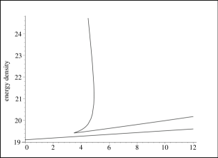
Figure 1: Ground state energy density vs. $g^{2}Q_{ave}^{2}$. $L=31$, and $\eta=0.1$. The lower line is the ground state energy density of $H_{W}$, Eq. (47).

In Fig. 1 we show this ground state energy density when $L=31$ and $\eta=0.1$. The parameters $\xi$ and $\tau$ are chosen so $N_{ave}=0.5$, and $g^{2}Q^{2}_{ave}$ takes a value on the abscissa of Fig. 1. The lower branch of the cusped curve is the ground state energy density produced by our basis. To obtain the energy density at the gauge invariant limit, we fit a quadratic curve to the lower branch of the cusped curve, requiring that the curves intersect at the points $g^{2}Q_{ave}^{2}=$5.02, 5.00 and 4.98. The energy density on this curve at $g^{2}Q_{ave}^{2}=0$ is our extrapolant: ${\cal E}=19.1192$, which is to be compared with the true ground state energy density ${\cal E}_{0}$=19.1008. The fractional error is 0.000974. Very similar results are obtained when the quadratic curve is fitted to the lower branch of the cusped curve at other points. The probability of “overexcitation” of a color/link degree of freedom is in the range 0.11 to 0.12 for the ground states parameters that produce the lower branch of the cusped curve.

Fig. 2 shows the ground state energy density when $L$ and $\eta$ are larger. The extrapolated and true ground state energy densities are ${\cal E}=19.2356$ and ${\cal E}_{0}=19.1008$ for a fractional error 0.00706.

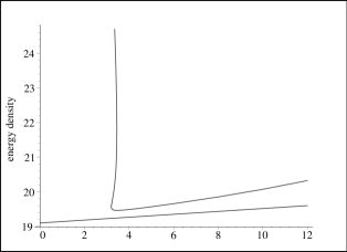
Figure 2: Ground state energy density vs. $g^{2}Q_{ave}^{2}$. $L=51$, and $\eta=0.5$.

The ground state energy curve when $\eta=.01$ resembles Fig. 1, but the cusp is more pronounced. In this case, the fractional error of the extrapolant is 0.000316 when $L=31$. We conclude that the results for the ground state are stable when $\eta$ is scaled by a factor of 50.

IV.2 The Basis and Excited States

The numerical data for the excited basis states is most easily explained by laying out a typical example. Consider the basis when $L=31$ and $\eta=0.1$. We take $\tau=0.428886$ and $\xi=0.0567920$, which sets $N_{ave}$=0.5 and $g^{2}Q^{2}_{ave}=4.000$, on the lower branch of Fig. 1. The basis consists of 815 single longitudinal pair states, and one single transverse pair state. The transverse state energy is independent polarization $s$, so in fact it is doubly degenerate, corresponding to the two-fold degeneracy we found for the spin zero eigenstates of $H_{W}$. These states all lie in the energy interval $0.252337\leq E\leq 0.470661$ above the ground state. Our convention is to order the states with increasing energy, with the ground state assigned ordinal number zero. Then when $g^{2}Q^{2}_{ave}=4.000$, the transverse pair state has ordinal number 777, and its energy is 0.447724.

The basis energies vary with $g^{2}Q^{2}$, and Fig. 3 shows seven states near $g^{2}Q_{ave}^{2}=4.000$. The longitudinal pair states never cross each other, but the transverse pair state crosses four longitudinal pair states in the region depicted. The level crossings are consistent with the fact that the longitudinal pair energies and the transverse pair energy are directed toward different limits as $g^{2}Q_{ave}^{2}$ is reduced.

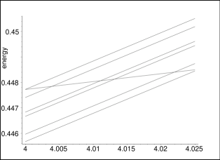
Figure 3: Excited state energy (above ground state) vs. $g^{2}Q_{ave}^{2}$, for eigenstates of $G_{C}$. Ordinal states 772 to 778 are shown.

We next repeat the computations of the energies when $g^{2}Q^{2}_{ave}=4.000\pm 0.0200$, fit quadratic curves through the three data points and extrapolate to $g^{2}Q^{2}_{ave}=0$. The extrapolated energies of all 815 longitudinal pair states are very close to zero. For example, ordinal state 100 has energy 0.313099 at $g^{2}Q^{2}_{ave}=4.000$. The extrapolated energy is -0.0110660. To merge with the ground state, the extrapolated energy would have to be zero. The fractional error is about -0.035. As the ordinal quantum number of the longitudinal pair increases, the extrapolated energy of the longitudinal pair also increases. The range over all 815 longitudinal pairs is from -0.023 to +0.017. Thus, to accuracy we might expect, the longitudinal states merge with the ground state at $g^{2}Q^{2}_{ave}=0$. For the transverse state, however, the extrapolated energy is 0.3788, which should be compared to the exact result 0.4047 (from $H_{W}$) on this lattice.

Table 1: Extrapolated first excited tranverse pair energy. Exact energy is 0.4047. For each value of $g^{2}Q^{2}_{ave}$ the top entry occurs when the transverse pair is near the top of the longitudinal pair basis, as indicated by the ordinal number.

$g^{2}Q^{2}_{ave}$:	4.000	5.000	7.000
$\eta$
0.043	–	–	0.3552
0.070	–	0.3843	0.3379
0.095	0.3805	0.3743	0.3236
0.100	0.3788	0.3723	0.3236
0.300	0.3076	0.3024	0.2453
0.500	0.2483	0.2516	0.2018

Table 2: Extrapolated second excited tranverse pair energy. Exact energy is 0.5723.

$g^{2}Q^{2}_{ave}$:	4.000	5.000	7.000
$\eta$
0.070	–	–	0.5490
0.100	–	–	0.5357
0.115	–	0.5692	0.5259
0.190	0.5501	0.5493	0.4900
0.300	0.5232	0.5174	0.4456
0.500	0.4725	0.4630	0.3848

The most interesting issue is how close the extrapolated transverse pair energies approach exact results when we vary $\eta$ and the $g^{2}Q^{2}_{ave}$ from which we start the extrapolation. These results are given for the two lowest energy transverse pair states in Tables 1 and 2. Some table entries are empty because when $\eta$ is sufficiently small, even the lowest transverse pair states lie above the band of longitudinal pair states. That is, they are not in the basis as we have defined it. The top entry in each column is for a value of $\eta$ where the transverse pair state falls just below the highest energy longitudinal pair states in the the basis, as indicated.

The next question is how to select a prediction, since the table entries vary considerably. For a given column in the tables we choose the entry with the smallest value of $\eta$, since this parameter fixes the strength of the term $g^{2}\eta Q^{2}_{0}$ in $G_{B}$, which perturbs the basis states relative to the eigenstates of $H_{A}$. For each column, this selects the largest entry in the column. Given that, it is natural to select the largest entry in the table as the prediction. The fractional error of this prediction for the first excited pair state is then (0.3843-0.4047)/0.4047=-0.050. For the second excited pair state the fractional error is -0.005, and for the third excited pair state the error is +0.002.

In the next section we will see that the reliability of these extrapolations for transverse pair states is crucial for our approach to pure SU(3) lattice gauge theory.

V Eigenstates of the Hamiltonian

The basis consists of one pair eigenstates of $G_{C}$, to which operator we must add the interaction term $=-\xi N^{\prime}$ to obtain Hamiltonian $H_{B}$. On our basis, the interaction term is a rank one operator. It may be written

$$-\xi N^{\prime} = -(384)\xi A({\bf k})\sum_{s=1}^{3}\sum_{\bf k}N_{2,s}({\bf k})$$

$$\times \{|{\bf k},s\rangle\langle 0|+|0\rangle\langle{\bf k},s|\}.$$

The sums are over the seed momenta only.

We can immediately write half the transverse eigenstates of $H_{B}$. Recall that the states $|{\bf k},s\rangle$ with $s=1,2$ are degenerate eigenstates of $G_{C}$. This means that the orthonormal combinations

$$|{\bf k},\pm\rangle=\frac{1}{\sqrt{2}}\left\{|{\bf k},1\rangle\pm|{\bf k},2\rangle\right\}$$ (78)

are also eigenstates with the common eigenvalue. However, it is evident that $(-\xi N^{\prime})|{\bf k},-\rangle=0$, so the $|{\bf k},-\rangle$ states are already eigenstates of $H_{B}$. This means the predications we extracted from Tables 1 and 2 are extrapolated eigenvalues of both $G_{C}$ and $H_{B}$ for these states. The remaining task, then, is to see whether the states $|0\rangle$, $|{\bf k},+\rangle$ and $|{\bf k},L\rangle$, which are connected by operator $-\xi N^{\prime}$ form gauge invariant eigenstates of $H_{B}$ that extrapolate to the limits in Tables 1 and 2.

Because $-\xi N^{\prime}$ is a rank one operator on our basis, it is easy to construct eigenstates of $H_{B}$ despite the large size of the basis. Let $|n\rangle$ denote a pair state belonging to our basis, and let $E_{n}$ be the corresponding eigenvalue of $G_{C}$. An eigenstate of $H_{B}$ will be a linear combination of our basis states:

$$|\psi\rangle=\alpha|0\rangle+\sum_{n}\beta_{n}|n\rangle.$$ (79)

Then the eigenvalue equation

$$H_{B}|\psi\rangle=(G_{C}-\xi N^{\prime})|\psi\rangle={\cal E}|\psi\rangle$$ (80)

leads to the relations

$$\beta_{n} = \frac{\langle n|(-\xi N^{\prime})|0\rangle}{{\cal E}-E_{n}}\alpha,$$ (81)

$${\cal E}\alpha = \sum_{n}\langle 0|(-\xi N^{\prime})|n\rangle\beta_{n}.$$ (82)

Substituting the first expression into the second, we obtain the eigenvalue equation

$${\cal E}=\sum_{n}\frac{|\langle 0|(-\xi N^{\prime})|n\rangle|^{2}}{{\cal E}-E_{n}}.$$ (83)

It is easy to locate the solutions of the eigenvalue equation. Suppose the basis eigenvalues $E_{n}$ are labeled so they increase monotonically with $n$. Then as ${\cal E}$ increases through the interval $[E_{n},E_{n+1}]$, the right side of Eqn. (83) decreases monotonically from $+\infty$ to $-\infty$. As ${\cal E}$ varies in this way, the left side increases monotonically. Thus, there is one solution of the eigenvalue equation in the interval. In addition to these solutions, there is one solution below ${\cal E}=0$, the new ground state, and one solution above the largest $E_{n}$.

Fig. 4 shows the eigenstates of $H_{B}$ in the region of the spectrum displayed in Fig. 3, again on a lattice with $L=31$, $\eta=0.1$. In keeping with the quantum mechanical result that interacting states do not cross, states approach each other closely, but never cross. For this reason, there can no longer be a distinct transverse polarization state. However, there is still a trace of the transverse basis state. By comparing Figs. 3 and 4, we can see how trajectories of eigenstates of $H_{B}$ bend to follow the path of the transverse basis state. Two observations explain why this happens. First, when a transverse basis state crosses a longitudinal basis state, there must be an eigenstate of $H_{B}$ with ${\cal E}=E_{L}=E_{T}$. (The eigenvector is a linear combination of the two crossing basis states.) Between such intersections, eigenvalue equation (83) still has a solution close the $E_{T}$ because in this regime, $|\langle 0|(-\xi N^{\prime})|T\rangle|^{2}|/\langle 0|(-\xi N^{\prime})|L\rangle|^{2}\sim 0.1$.

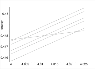
Figure 4: Excited state energy (above ground state) vs. $g^{2}Q_{ave}^{2}$, for eigenstates of $H_{B}$ Ordinal states 772 to 777 are shown.

The eigenvalues of $H_{B}$ extrapolate to limits very close to zero, and all but two of them behave like nearby eigenvalues of $G_{C}$. We mentioned that ordinal eigenvalue 100 of $G_{C}$ extrapolates $0.313099\rightarrow-0.0110660$. Ordinal eigenvalue 100 of $H_{B}$ extrapolates $0.313132\rightarrow-0.0110627$.

However, two eigenvalues are bizarre. At $g^{2}=4.000$, the new ground state is ${\cal E}_{0}=-64.9678$. Note that the interaction $-\xi N^{\prime}$ is a traceless operator on our basis, so the sum of eigenvalues $\cal E$ is the same as the sum of the $E_{n}$. This suggests that a very positive eigenvalue is to be found. Sure enough, ${\cal E}_{816}=+65.3527$. The next lower eigenvalue is ${\cal E}_{815}=0.47064$, sandwiched between $E_{815}$ and $E_{816}$.

The very positive eigenvalue is an artifact of the cutoff of the basis. For example, if we omit basis state 816, then it is ${\cal E}_{815}$ that is very large. Because of the tracelessness of the interaction, the cutoff of the basis also induces the very negative ${\cal E}_{0}$.

This pathology largely disappears when we extrapolate. For ${\cal E}_{0}$, the extrapolation is $-64.9678\rightarrow 0.134561$; for ${\cal E}_{816}$, the extrapolation is $+65.3527\rightarrow-0.137485$. The fractional deviation of the extrapolated ground state energy from zero is +0.002. We will take zero to be the extrapolated energy for all these energy levels.

But if all energy levels extrapolate to zero within expected accuracy, what became of the gauge invariant basis state that extrapolated near energy 0.4047? At this point, the evidence we have of its presence is that eigenstates of $H_{B}$ take turns following the trajectory of the transverse basis state.

This picture is clarified when we follow the “locus of gauge invariance,” as we vary $g^{2}Q^{2}_{ave}$. The expectation value of the operator $g^{2}Q^{2}$ in the eigenstates of $G_{C}$ or $H_{B}$ may be expressed

$$\langle|g^{2}Q^{2}|\rangle=L^{3}g^{2}Q^{2}_{ave}+\Delta.$$ (84)

A gauge invariant state results when we take the limit $g^{2}Q_{ave}\rightarrow 0$ and find $\Delta=0$ in the limit.

Consider $\Delta$ for the basis states, the eigenstates of $G_{C}$. A transverse basis state has $\Delta=0$ at all values of $q^{2}Q^{2}_{ave}$, and so when we extrapolate this variable to zero, the transverse basis states become gauge invariant. The basis states $|{\bf k},-\rangle$, share this property, and we have seen that they are eigenstates of $H_{B}$ as well as $G_{C}$.

Among the other eigenstates of $H_{B}$, however, no one state has $\Delta=0$, at nonzero $g^{2}Q^{2}_{ave}$ For these states, $\Delta$ varies with $g^{2}Q^{2}_{ave}$. We find there is an abrupt dip in $\Delta$ where the state follows the transverse basis state, that is, when $g^{2}Q^{2}_{ave}$ is adjusted so ${\cal E}\sim E_{T}$. This dip is explained by Eq. (81), which shows that the amplitude of the transverse state in the eigenstate is particularly large in this region of $g^{2}Q^{2}_{ave}$.

This behavior is illustrated in Fig. 5. $\Delta$ dips to a minimum less than 2% of its asymptotic value. Fig. 4 confirmes that the dip occurs when $g^{2}Q^{2}_{ave}$ is in the interval where ordinal state 773 follows the transverse basis state trajectory.

As successive states follow the transverse basis state trajectory, the “locus of gauge invariance” passes from one eigenstate to the next, always close to the transverse basis state. This transition process is shown in Fig. 6, where the dips for states 772 through 777 are shown together. Note that dips in $\Delta$ intersect where $\Delta$ is half its asymptotic value. At an intersection, the normalized probability of finding the transverse basis state in the eigenstate, $|\beta_{T}|^{2}$, is about 1/2 for each of the “dipping” states. (The sum of the probabilities over all the eigenstates of $H_{B}$ is one.) At an intersection of dips, the “locus” passes from one eigenstate to the next.

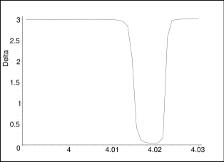
Figure 5: $\Delta$ vs. $g^{2}Q^{2}_{ave}$. This is for ordinal state 773. The dip occurs where the state follows the trajectory of the transverse basis state.

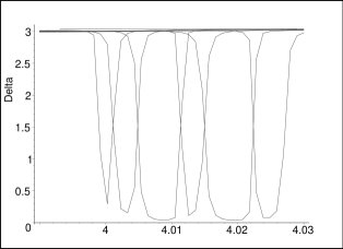
Figure 6: $\Delta$ vs. $g^{2}Q^{2}_{ave}$. Dips for ordinal states 772 (on right) through 777 (on left) are superposed.

Thus, the “locus of gauge invariance” follows the transverse basis state. This conclusion is guaranteed by Eq. (81). The extrapolation of this picture to $g^{2}Q^{2}_{ave}=0$ is provided by Table 1. This is as close as we can come to the verification that there is a second spin 0 gauge invariant state at energy 0.3843, thereby confirming double degeneracy of the spin zero gauge invariant states.

VI Conclusion

We now consider how the methods we have developed can be applied to pure SU(3) lattice gauge theory at general coupling. In this case, all the terms in Eqs. (52) and (III) contribute to $H_{A}$. The “chromoelectric” operators ${\cal J}^{2}$ each produce terms which are a product of up to four $A$’s and $A^{\dagger}$’s. The “chromomagnetic” operators ${\rm Tr}(UUU^{\dagger}U^{\dagger})$ each produce terms which are a product of up to eight. The operator $g^{2}Q^{2}$ produces terms which are a product of up to four such factors.

Terms having more than two factors are interaction-type, and are not present in the weak coupling limit we have been studying.

The generator $G_{B}$ is now constructed from the terms in $H_{A}$ and $g^{2}Q^{2}$ that are no more than quadratic in $A$’s and $A^{\dagger}$’s, using Eq. (18). The basis is chosen from the low energy, one pair eigenstates of this generator.

The main complication beyond those we have studied comes from the fact that the expression for $H_{B}$, Eq. (19), now has interaction terms on the right side. When these terms are added to $-\xi N$, the resulting interaction term is no longer a rank one operator. Therefore, the construction of the eigenstates of $H_{B}$ is more complex than it is for the weak coupling case we have studied.

Interaction terms may pose a technical challenge, but they are required if our approach is to produce states like glueballs on the lattice. To see this, note that Eq. (12) implies that a pair state is an excitation in which the amplitude for the excitation of two links has the spatial dependence $e^{2\pi i{\bf k\cdot\Delta s}/L}$, where $\bf\Delta s$ is the distance between the links. The magnitude of this amplitude is independent of $|{\bf\Delta s}|$. In a glueball, on the other hand, the amplitude falls off in magnitude when $|{\bf\Delta s}|$ is more than the diameter of the glueball. Such behavior can be approximated when the eigenstates of $H_{B}$ are superpositions of many pair states, which in turn requires that there be interaction terms between pair states.

One concern is that there may not be enough basis pair states to superpose to make a glueball. There are always many longitudinal polarization pair states in a basis, but that is not true for transverse pair states. An extreme example is provided by the case we have used extensively in this paper, a lattice with $\eta=0.1$ and $g^{2}Q^{2}_{ave}\sim 4.0$. For these parameters, there are 815 longitudinal polarization pair states and just one transverse pair momentum. (There are two degenerate states, one for each transverse polarization.) To get more transverse states in the basis, we increase $\eta$, which increases the energy interval between longitudinal pair states. Table 3 lists the number of longitudinal and transverse pair states for different values of $g^{2}Q^{2}_{ave}$, when $\eta=0.5$. These results are for the weak coupling generator, but they suggest that it will be possible construct a basis with many transverse polarization states.

Table 3: Number of longitudinal (L) and transverse (T) seed momenta in bases having different $g^{2}Q^{2}_{ave}$. $\eta=0.5$.

$g^{2}Q^{2}_{ave}$:	4.000	6.000	8.000	10.000
L	108	113	113	112
T	4	9	18	30

It should be remembered that adding states to a basis can only improve the accuracy of the approximate eigenvalues we compute. Thus we are not obliged to slavishly follow the rules we have set forth for a basis. One can add further transverse pairs having energies greater than the highest energy longitudinal pairs to improve the “localization ” of glueballs. One of the attractive features of a variational basis is that ideas like this can be tried.

These considerations set the stage for the exploration of the general coupling case, which is the goal of this line of research. However, the exploration lies beyond the scope of this paper.

References

- (1) J. B. Bronzan and Yüksel Gunal, Phys. Rev. D 5̱0, 5924 (1994).
- (2) J. Kogut and L. Susskind, Phys. Rev. D 11, 395 (1975).
- (3) M. Loan, X.-Q. Luo and Z.-H. Luo, Int. J. Mod. Phys. A21, 2905 (2006).
- (4) C. Itzykson and J.-B. Zuber, Quantum Field Theory (McGraw-Hill, New York, 1980), p. 516.
- (5) J. B. Bronzan, Phys. Rev. D 40, 3493 (1989).
- (6) J. B. Bronzan and T. E. Vaughan, Phys. Rev. D 44 3264 (1991).
- (7) J. J. deSwart, Rev. Mod. Phys. 35, 916 (1963).
- (8) V. F. Muller and W. Ruhl, Nucl. Phys. B230, 49 (1984).
- (9) J. B. Bronzan, Phys. Rev. D 31, 2020 (1985).
- (10) G. F. Koster, Space Groups and their Representations (Academic Press, New York, 1957), p. 21.