Analytical continuation from imaginary to real chemical potential in 2-color QCD under scrutiny

Abstract:

The method of analytical continuation from imaginary to real chemical potential is tested in 2-color QCD. In comparison to previous studies in the same theory, an exact updating algorithm is used and simulations are performed closer to the thermodynamic limit. It is shown that the method considerably improves if suitable functions are used to interpolate data with imaginary chemical potential.

1 Introduction

The identification of the phases of QCD in the temperature – chemical potential plane and the exact localization and nature of the transitions among them are of central interest nowadays, due to the implications in cosmology, in astrophysics and in the phenomenology of heavy ion collisions. Most aspects of the QCD phase diagram are beyond the reach of perturbation theory and the lattice approach is a natural tool to face them. For non-zero chemical potential, however, the QCD fermion determinant becomes complex and the standard Monte Carlo importance sampling is unfeasible – the well-known “sign problem”.

Several strategies have been invented to circumvent this problem (for a review, see [1] and [2]) and some useful information on the critical line separating the hadronic phase from the quark-gluon plasma phase in the region $\mu/T\lesssim 1$ has been already achieved.

Here, we concentrate on one of these approaches, the method of analytical continuation, first used in Ref. [3] and in Ref. [4]. The idea behind this method is very simple: numerical simulations are performed at imaginary chemical potential, $\mu=i\mu_{I}$, for which the fermion determinant is real, then Monte Carlo determinations are interpolated by a suitable function and finally this function is analytically continued to real values of $\mu$. This method is rather powerful since $\beta$ and $\mu$ parameters can be varied independently and there is no limitation from increasing lattice size, as in methods based on reweighting. There is, however, an important drawback: the periodicity of the partition function and the presence of non-analyticities arising for imaginary values of the chemical potential [5] make that the region useful for numerical determinations is inside the strip $0\leq\mu_{I}/T<\pi/3$. This implies that the accuracy in the interpolation of the results at imaginary chemical potential has a strong impact on the extension of the domain of real $\mu$ values reachable after analytical continuation.

So far, the method of analytical continuation has been applied in SU(3) with $n_{f}=2$ [6], $n_{f}=3$ [7] and $n_{f}=4$ [8]. Moreover, it has been tested in several theories which do not suffer the sign problem, by direct comparison of the analytical continuation with Monte Carlo results obtained at real $\mu$ [4, 9, 10].

In all these applications a truncated Taylor series (or, more simply, a polynomial) has been used as interpolating function. In this work we show that the method can be considerably improved if ratios of polynomials are used instead. As a test-field for our proposal we adopt the same theory used in Ref. [9], namely SU(2) (or 2-color QCD), with $n_{f}=8$ degenerate staggered fermions.

2 Theoretical background

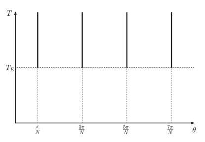
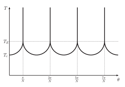
Figure 1: (Left) Phase diagram in the $(T,\theta)$ plane according to Ref. [5]. (Right) Tentative phase diagram in the $(T,\theta)$ plane after the inclusion of the chiral critical lines.

Long ago Roberge and Weiss have shown [5] that the partition function of any SU($N$) gauge theory with non-zero temperature and imaginary chemical potential, $\mu=i\mu_{I}$, is periodic in $\theta\equiv\mu_{I}/T$ with period $2\pi/N$ and that the free energy $F$ is a regular function of $\theta$ for $T<T_{E}$, while it is discontinuous at $\theta=2\pi(k+1/2)/N$, $k=0,1,2,\ldots$, for $T>T_{E}$, where $T_{E}$ is a characteristic temperature, depending on the theory. The resulting phase diagram in the $(T,\theta)$-plane is given in Fig. 1 (left), where the vertical lines represent first order transition lines. This structure is compatible with the $\mu\to-\mu$ symmetry, related with CP invariance, and with the Roberge-Weiss periodicity. The $\mu_{I}$-dependence of any observable is completely determined if this observable is known in the strip $0\leq\theta<\pi/N$. These predictions have been confirmed numerically in several cases, studying the behaviour of quantities like the Polyakov loop and the chiral condensate [6, 8, 9].

A phase diagram like that in Fig. 1 (left) would imply the absence of any transition along the $T$ axis in the physical regime of zero chemical potential for any value of $N$, of $n_{f}$ and of the quark masses, which cannot be true. Therefore, it is necessary to admit that the phase diagram in the $(T,\theta)$-plane is more complicated than in Fig. 1 (left). The simplest possibility is given in Fig. 1 (right), where the added lines generally represent transitions which can be first order, second order or crossover. The temperature $T_{c}$ is the critical or pseudo-critical one for the transition at zero chemical potential. It is convenient to redraw the phase diagram of Fig. 1 (right) in the $(\beta,\hat{\mu}_{I})$-plane (Fig. 2), where $\beta=2N/g^{2}$, $\hat{\mu}_{I}=a\mu_{I}$ is the imaginary chemical potential in lattice units and it has been used the fact that $T=1/(aN_{\tau})$, with $N_{\tau}$ the temporal extension of the lattice.

3 Numerical results

We performed numerical simulations on a $16^{3}\times 4$ lattice of the SU(2) gauge theory with $n_{f}=8$ degenerate staggered fermions having mass $am=0.07$. For this theory the tentative phase diagram looks like in Fig. 2, with $\beta_{E}\simeq 1.55$ [9] and $\beta_{c}\simeq 1.41$[11]. We used the hybrid Monte Carlo algorithm, with $dt=0.01$. The observables we determined are the Polyakov loop, the chiral condensate and the fermionic number density. We have chosen $\beta=1.90>\beta_{E}$ and have taken 1000-5000 measurements for several values of the imaginary chemical potential $\mu_{I}$ in the interval from zero to the value corresponding to the first RW transition line, $\hat{\mu}_{I}=\pi/8$, and for several values of the real chemical potential $\mu_{R}$ in the interval $[0,2]$. Simulations have been performed on the APEmille crate in Bari and on the recently installed computer facilities at the INFN apeNEXT Computing Center in Rome.

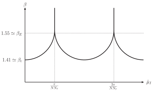
Figure 2: Phase diagram in the $(\beta,\hat{\mu}_{I})$-plane; $N$ is the number of colors, $N_{\tau}$ the extension of the lattice in the temporal direction. The numerical values for $\beta_{E}$ and $\beta_{c}$ are valid for SU(2) in presence of $n_{f}=8$ degenerate staggered fermions with mass $am=0.07$.

We have used the data at imaginary chemical potential $\mu_{I}$ to determine the parameters of the interpolating function, then we have analytically continued this function to real values of the chemical potential and compared there with direct Monte Carlo determinations. In order to fulfill CP invariance, the interpolating function must be a function of $\mu^{2}$ for observables, such as the Polyakov loop and the chiral condensate, which do not depend explicitly on $\mu$. The fermion number density, being the logarithmic derivative of the partition function with respect to the chemical potential, is instead an odd function of $\mu$. For the Polyakov loop and the chiral condensate we have considered a second order polynomial in $\mu^{2}$,

$$A+B\mu^{2}+C\mu^{4}\;,$$ (1)

according to the standard approach, and the ratio of two first oder polynomials in $\mu^{2}$,

$$\frac{A+B\mu^{2}}{1+C\mu^{2}}\;,$$ (2)

according to our new proposal. Similarly, for the fermionic number density we have used a polynomial of the form

$$A\mu+B\mu^{3}+C\mu^{5}\;,$$ (3)

and the ratio

$$\frac{A\mu+B\mu^{3}}{1+C\mu^{2}}\;.$$ (4)

Our findings are summarized in Figs. 3, 4 and 5. In Fig. 3 we put on the same plot the imaginary part of the fermionic number density as a function of $\mu_{I}$ and the real part of the fermionic number density as a function of the real $\mu$. The two data sets match smoothly in $\mu=0$, which is a necessary condition for the applicability of the method of analytical continuation. The fermionic density approaches 2 for large values of the real chemical potential. This saturation effect is artificial and is due to the fact that no more than two fermions per site can be accommodated in the lattice (“Pauli blocking”). The solid lines represent the two kinds of interpolating functions, whose parameters are determined by a fit on the data at imaginary chemical potential. Here both interpolations, polynomial and rational function, nicely reproduce the data at real $\mu$ over a large interval. Deviations start at values of $\mu$ for which the saturation effects are certainly important.

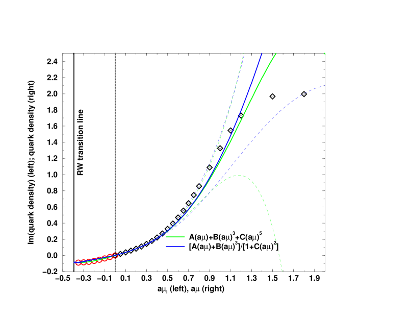
Figure 3: Negative side of the horizontal axis: imaginary part of the fermionic number density vs. the imaginary chemical potential. Positive side of the horizontal axis: real part of the fermionic number density vs. the real chemical potential. The green (blue) solid lines represent the polynomial (ratio of polynomials) interpolating function; the dashed lines give the corresponding uncertainty, coming from the errors in the parameters of the fit.

In Fig. 4 we show the chiral condensate as a function of $\mu^{2}$. Again data at imaginary $\mu$, i.e. $\mu^{2}<0$, and data at real $\mu$, i.e. $\mu^{2}>0$, nicely match at $\mu=0$. This time the different behavior of the two kinds of interpolation clearly emerges. The ratio of first order polynomials in $\mu^{2}$ reproduces the data at real $\mu$ on a much larger interval than the second order polynomial in $\mu^{2}$. Deviations arise for values of real $\mu$ for which saturation effects are probably already important. The same conclusions can be drawn from Fig. 5 which shows data and interpolations for the Polyakov loop.

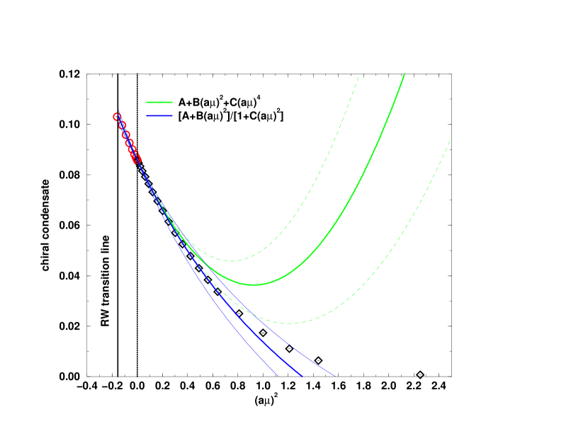
Figure 4: Chiral condensate vs. $\mu^{2}$. The solid and dashed lines have the same meaning as in Fig. 3.

The above conclusions do not change if larger order terms are included in the polynomial interpolation (1). In fact, larger order polynomials fail to reproduce the data at real $\mu$ even earlier in $\mu$ than second order polynomials. This is due to the fact that the higher order terms of the polynomial are the less accurately determined in the fit to data at imaginary $\mu$. On the other side, if in the ratio of polynomials the order of the polynomials at the numerator and/or at the denominator is increased, no improvement is observed.

An approach alternative to that based on ratio of polynomials is to use large order polynomials and then to build out of them rational functions by means of Padé approximants. This alternative approach behaves in a way comparable to ratio of polynomials.

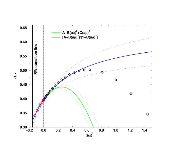
Figure 5: Polyakov loop vs. $\mu^{2}$. The solid and dashed lines have the same meaning as in Fig. 3.

4 Conclusions and outlook

We have verified by comparison with direct Monte Carlo determinations at real chemical potential in 2-color QCD that the method of analytical continuation considerably improves if ratio of polynomials is used as interpolating function instead of truncated Taylor series.

In the case of the Polyakov loop and of the chiral condensate an interpolation of numerical data at imaginary chemical potential over the window permitted by Roberge-Weiss singularities allows an extrapolation to real values of the chemical potential over a much larger region.

Deviations at very large values of the chemical potential could be due to unphysical saturation of the fermionic density (“Pauli blocking”).

References

- [1] O. Philipsen, PoS LAT2005 (2006) 16, [arXiv:hep-lat/0510077].
- [2] C. Schmidt, these proceedings.
- [3] M.P. Lombardo, Nucl. Phys. (Proc. Suppl.) 83 (2000) 375.
- [4] A. Hart, M. Laine and O. Philipsen, Phys. Lett. B505 (2001) 141.
- [5] A. Roberge and N. Weiss, Nucl. Phys. B275 (1986) 734.
- [6] P. de Forcrand and O. Philipsen, Nucl. Phys. B642 (2002) 290; Nucl. Phys. (Proc. Suppl.) 119 (2003) 535 [arXiv:hep-ph/0301209].
- [7] P. de Forcrand and O. Philipsen, Nucl. Phys. B673 (2003) 170; Nucl. Phys. (Proc. Suppl.) 129 (2004) 521, [arXiv:hep-lat/0309109].
- [8] M. D’Elia and M.P. Lombardo, arXiv:hep-lat/0205022; Phys. Rev. D67 (2003) 014505; Nucl. Phys. (Proc. Suppl.) 129 (2004) 536 [arXiv:hep-lat/0309114].
- [9] P. Giudice and A. Papa, Phys. Rev. D69 (2004) 094509.
- [10] S. Kim, Ph. de Forcrand, S. Kratochvila, T. Takaishi, PoS LAT2005 (2006) 166 [arXiv:hep-lat/0510069].
- [11] Y. Liu, O. Miyamura, A. Nakamura and T. Takaishi, [arXiv:hep-lat/0009009].
- [12] M.P. Lombardo, PoS LAT2005 (2006) 168 [arXiv:hep-lat/0509181].