Improvement of algorithms for dynamical overlap fermions

Abstract:

We investigate the algorithms for dynamical overlap fermions aiming at improving the performance for large-scale simulations. We look for the best combination of Hybrid Monte Carlo options and iterative quark solvers with respect to the numerical costs. Our main target is a $N_{f}=2$ simulation with overlap fermion on a $16^{3}\times 32$ lattice at lattice spacing around 0.12 fm.

1 Introduction

The JLQCD Collaboration is performing dynamical QCD simulations with the overlap fermions, as a new project started in 2006 [1, 2, 3, 4]. At present, our main run is generating lattices of size $16^{3}\times 32$, $a\simeq 0.12$ fm, with two flavors of sea quarks whose smallest mass $\simeq m_{s}/6$. The topological sector is fixed by a pair of extra Wilson fermions. This considerably improves the efficiency of the HMC algorithm, while the effect of fixing the topological charge $Q$ should be examined by measuring on configurations with different values of $Q$. Numerical simulations at different values of $Q$, as well as with larger lattices and with $2+1$ flavors, are also in preparation.

These studies are being carried out on a new supercomputer system at KEK, which is in service since March 2006 [5]. The system has two computational servers: Hitachi SR11000 model K1 (peak performance 2.15TFlops), and IBM System Blue Gene Solution (57.3TFlops). The latter system has 10 racks, each composed of 1024 nodes (2048 processor cores). For the Wilson fermion solver, with data on cache, the Blue Gene system achieves about 29% of the peak performance on a half-rack system.

Even on these powerful machines, the dynamical overlap simulation is quite challenging. The simulation is performed with the Hybrid Monte Carlo (HMC) algorithm. In this paper, we describe our attempt to speed-up the simulation by improving the HMC algorithms.

2 Action

The effective action we treat in the HMC simulation has a form,

$$S=S_{G}+S_{F}+S_{E}.$$ (1)

$S_{G}$ is the gauge field part, for which we adopt the renormalization group improved (Iwasaki) action, while in an exploratory stage of this work a modified plaquette gauge action, which is designed to suppress dislocations, was also investigated [3].

As the quark action, we use the $N_{f}=2$ overlap fermion action. The overlap-Dirac operators is represented as

$$D(m)=\left(m_{0}+\frac{m}{2}\right)+\left(m_{0}-\frac{m}{2}\right)\gamma_{5}\,\mbox{\rm sign}(H_{W}),$$ (2)

where $H_{W}=\gamma_{5}D_{W}$, $D_{W}$ is the Wilson-Dirac operator with a large negative mass $-m_{0}$. The sign function in Eq. (2) is approximated by a partial fraction form [7, 8]:

$$\mbox{\rm sign}(H_{W})=\frac{H_{W}}{\sqrt{H_{W}^{2}}}\simeq H_{W}\left(p_{0}+\sum_{l=1}^{N}\frac{p_{l}}{H_{W}^{2}+q_{l}}\right).$$ (3)

The $N$ inversions $(H_{W}^{2}+q_{l})^{-1}$ are calculated at the same time using the multi-mass conjugate gradient method.

We utilize the mass preconditioning [6], i.e. introducing a preconditioning term with heavier quark mass $m^{\prime}$ than that of the dynamical quark. The fermion action becomes $S_{F}=S_{PF1}+S_{PF2}$,

$$S_{PF1}=\phi_{1}^{\dagger}[D(m^{\prime})^{\dagger}D(m^{\prime})]^{-1}\phi_{1},\hskip 8.5359ptS_{PF2}=\phi_{2}^{\dagger}\left\{D(m^{\prime})[D(m)^{\dagger}D(m)]^{-1}D(m^{\prime})^{\dagger}\right\}\phi_{2},$$ (4)

where $S_{PF1}$ is the preconditioner and $S_{PF2}$ is the preconditioned dynamical quark term with corresponding pseudofermion fields $\phi_{1}$ and $\phi_{2}$, respectively.

$S_{E}$ is the extra Wilson fermion term defined as

$$\det\left(\frac{H_{W}^{2}}{H_{W}^{2}+\mu^{2}}\right)=\int{\cal D}\chi^{\dagger}{\cal D}\chi\exp[-S_{E}],$$ (5)

$$S_{E}=\chi^{\dagger}\left[(D_{W}+i\gamma_{5}\mu)(D_{W}^{\dagger}D_{W})^{-1}(D_{W}+i\gamma_{5}\mu)^{\dagger}\right]\chi,$$ (6)

where the denominator of Eq. (5) amounts to two flavors of heavy ghosts with a twisted mass $\mu$. This term suppresses near-zero modes of $H_{W}$, while keeping the effects on higher modes minimal [2, 9, 10, 11]. The newly introduced fields have mass of the order of lattice cutoff and therefore irrelevant in the continuum limit.

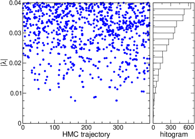
Figure 1: The low-lying modes of $H_{W}$ in the case with $S_{E}$ ($\mu=0.2$, left panel) and without $S_{E}$ (right panel) at $a\simeq 0.125$ fm and $m\simeq 2m_{s}$.

The quark action becomes singular when $H_{W}$ has a zero eigenvalue. This causes discontinuity in the conjugate momenta when $\lambda_{min}$ changes the sign during the molecular dynamics evolution. While this problem can be circumvented by the so-called reflection/refraction prescription [13], it requires monitoring of the near-zero eigenvalues and additional inversions of overlap operator, which largely increase the numerical cost. In our case, however, extra Wilson fermions prevent the near-zero mode from approaching zero, and hence these operations can be skipped.

How the extra Wilson fermions work is depicted in Figure 1. The figure compares appearance of low-lying eigenmodes during the HMC runs with and without $S_{E}$ at $a\simeq 0.125$ fm and $m\simeq m_{s}$. It is clear that $S_{E}$ suppresses the spectral density around $\lambda=0$. The same feature is found in the molecular dynamics history of the lowest mode displayed in Figure 2. With $S_{E}$, no reflection nor refraction occurs, contrary to the case without $S_{E}$. One can therefore switch off the monitoring of $\lambda$ in the case with $S_{E}$. Even when $\lambda=0$ occurs due to a finite molecular dynamics step size, it is signaled by large $\Delta H$ and thus rejected in the Metropolis test.

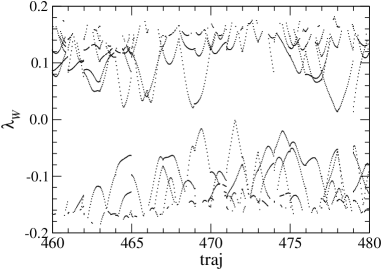
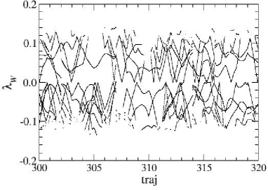
Figure 2: Evolution of $\lambda_{min}$ in the molecular dynamics at $a\simeq 0.12$ fm and $m\simeq 2m_{s}$. The left and right panels show the cases with and without $S_{E}$, respectively. The left panel shows an event that as if a reflection occurs, while is actually not the case.

3 Solver algorithms

Since the inversion of the overlap-Dirac operator is the most time consuming part of the HMC simulation, improvement of the solver algorithm is crucial. We compare two methods: the nested CG with relaxed precision of the inner CG loop, and the 5-dimensional CG algorithm.

The overlap operator requires computation of the partial fraction terms in Eq. (3). Therefore, the CG method to invert the overlap operator has a nested structure; the inner loop to calculate $(H_{W}^{2}+q_{l})^{-1}$, and the outer loop to operate $D(m)$. For the inner loop, the multi-shift CG method is used to solve $(H_{W}^{2}+q_{l})^{-1}$ for all $l$ simultaneously. The precision of the approximation Eq. (3) is determined by the degree $N$ and the condition number $\lambda_{max}/\lambda_{min}$. For a smaller $|\lambda_{min}|$, a larger $N$ is needed to keep the precision; e.g. $N$=10 corresponds to $O(10^{-7})$ accuracy for $|\lambda_{min}|$=0.05 and $O(10^{-5})$ for 0.01. The multi-shift CG method has an advantage that the cost is almost independent of $N$. Instead of extending the window $[|\lambda_{min}|,|\lambda_{max}|]$ for small $|\lambda_{min}|$, we may project out the low-lying modes explicitly and add back with the eigenvalue $\mbox{sign}(\lambda)$. In this way we may fix the lower limit of the approximation to some threshold $\lambda_{thrs}$, below which the eigenmodes are treated exactly.

The relaxed CG method is an improvement of the nested CG method. It changes the precision of the inner loop adaptively as the outer loop iteration proceeds [14]. As we will see, the relaxed CG is about twice faster than the original CG.

An alternative solver is the 5-dimensional CG method [15]. Let us consider the following form of a 5D matrix (an explicit example for the $N=2$ case):

$$M_{5}=\left(\begin{array}[]{cccc|c}H_{W}&-\sqrt{q_{2}}&&&0\\ -\sqrt{q_{2}}&-H_{W}&&&\sqrt{p_{2}}\\ &&H_{W}&-\sqrt{q_{1}}&0\\ &&-\sqrt{q_{1}}&-H_{W}&\sqrt{p_{1}}\\ \hline\cr 0&\sqrt{p_{2}}&0&\sqrt{p_{1}}&R\gamma_{5}+p_{0}H_{W}\\ \end{array}\right)=\left(\begin{array}[]{c|c}A&B\\ \hline\cr C&D\\ \end{array}\right).$$ (7)

Each component represents the usual 4D matrix. By the Schur decomposition,

$$M_{5}=\tilde{L}\tilde{D}\tilde{U}=\left(\begin{array}[]{cc}1&0\\ CA^{-1}&1\\ \end{array}\right)\left(\begin{array}[]{cc}A&0\\ 0&S\\ \end{array}\right)\left(\begin{array}[]{cc}1&A^{-1}B\\ 0&1\\ \end{array}\right),$$ (8)

where

$$S=D-CA^{-1}B=R\gamma_{5}+p_{0}H_{W}+H_{W}\sum_{i}\frac{p_{i}}{H_{W}^{2}+q_{i}}$$ (9)

expresses the partial fraction approximation of $D(m)$. Therefore, by solving

$$M_{5}\left(\begin{array}[]{c}\phi\\ \psi_{4}\\ \end{array}\right)=\left(\begin{array}[]{c}0\\ \chi_{4}\\ \end{array}\right),$$ (10)

$\psi_{4}=S^{-1}\chi_{4}$ is determined. A preconditioning is applied by multiplying the inverse of $M_{5}^{(0)}=M_{5}[U=0]$, which is easily inverted by forward and backward substitutions. The even-odd preconditioning is also applicable, and according to our performance comparison, this is the best solution for the 5D solver. Since the size of $M_{5}$ grows as $N$, the numerical cost increases linearly in $N$. A disadvantage is that the subtraction of low-modes of $H_{W}$ is not applicable when the even-odd decomposition is used. This causes a difficulty when $\lambda_{min}$ becomes too small to be approximated without the projection. To apply the 5D solver, one needs to determine the lowest boundary $V_{min}$ above which the partial fraction approximation is valid.

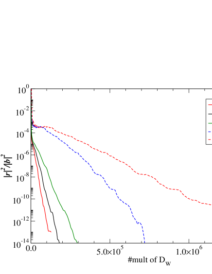
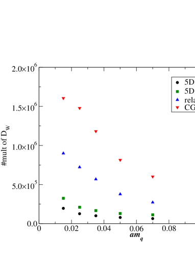
Figure 3: Comparison of the solver algorithms on a single configuration. The left panel shows convergence of the residue as the number of $D_{W}$ multiplication. The right panel shows quark mass dependence of the number of $D_{W}$ multiplication needed for $|r|^{2}/|b|^{2}<10^{-14}$.

Figure 3 shows the comparison of the solver algorithms at $a\simeq 0.12$ fm, $m\simeq 0.4m_{s}$, on a single configuration. The figure shows that the relaxed CG is factor of 2 faster than the standard CG method. The 5D solver is even faster by another factor of 2–3 than the relaxed CG for $N=20$. This conclusion is independent of the quark mass, as displayed in the right panel of Fig. 3. Therefore, if near-zero eigenvalues do not appear, as in the present case, the 5D solver is the fastest.

4 HMC algorithm

Multi-time step.

Magnitude of the forces corresponding to the terms, $S_{G}$, $S_{PF1}$, $S_{PF2}$, and $S_{E}$ has a hierarchical structure. In particular the gauge part has the largest contribution to the evolution of the conjugate momenta, while the cost to compute it is negligible compared to the fermionic part. The size of the force for $S_{PF2}$ is smaller compared to that of $S_{PF1}$. The multi-time step [12] makes use of this hierarchy by adopting different time steps for these terms in the molecular dynamical evolution.

The forces are compared in Fig. 4. This result suggest to chose the step sizes as

$$\Delta\tau_{(PF2)}\gg\Delta\tau_{(PF1)}\gg\Delta\tau_{(G)}=\Delta\tau_{(E)}.$$ (11)

While the size of the force for $S_{E}$ is as small as the fermionic part, $\Delta\tau_{(E)}$ is set to be the same as the gauge part, to ensure the disappearance of the near-zero modes, because the fluctuation of the $S_{E}$ force is large. The cost to determine the force of the extra Wilson fermions is negligible compared to the overlap fermion part. The ratio of the step sizes are determined by monitoring the size of the forces. For example, $\Delta\tau_{(PF2)}/\Delta\tau_{(PF1)}=5$ and $\Delta\tau_{(PF1)}/\Delta\tau_{(G,E)}=6$ are a reasonable choice for the displayed case.

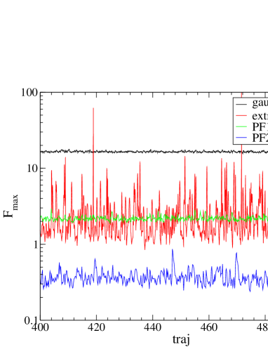
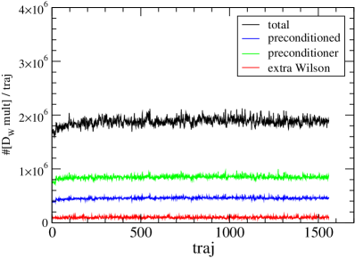
Figure 4: The maximum values of the forces (left panel) and the costs of the forces (right panel) monitored in HMC at $a\simeq 0.12$ fm and $m\simeq 2m_{s}$.

Noisy Metropolis test.

Considering the performance of the solvers in Sec. 3, the 5D CG method is preferable, with small number of poles $N$ if possible. As for the preconditioner, we can choose relatively small $N$, since the contributions to the dynamics cancel in $S_{PF1}$ and $S_{PF2}$. For $S_{PF2}$, one can also choose an $N$ with a less precise approximation by making use of the noisy Metropolis algorithm [16], which is prescribed as follows. At the end of a molecular dynamics evolution, after the usual Metropolis test, we accept $U_{new}$ with a probability $P=\min\{1,e^{-dS}\}$, where

$$dS=\left|\,W^{-1}[U_{new}]\,W[U_{old}]\,\xi\,\right|^{2}-|\xi|^{2},$$ (12)

$W=D(m)/D^{\prime}(m)$, with $D^{\prime}$ a less accurate overlap operator used in HMC, and $D$ the accurate overlap operator, $U_{old}$ is the initial gauge field, and $\xi$ is a random Gaussian noise vector.

Performance.

Finally, we show the present performance of HMC measured on the Blue Gene (512-node) at $a\sim 0.12$ fm, $\mu=0.2$, and a trajectory length $\tau=0.5$. The first three lines in Table 1 show the result for the simulation with the 4D (relaxed CG) solver, with which most of gauge configurations are generated so far. No noisy Metropolis test is incorporated. The last three lines in Table 1 show a preliminary result for the performance with fully improved algorithm, the less precise 5D solver in molecular dynamics with the noisy Metropolis test, which achieves about a factor of 3 acceleration. Therefore this algorithm is our current best option, which will be adopted in our productive run in future.

	$m_{ud}$	$m^{\prime}$	$N_{\tau(PF2)}$	$\frac{\Delta\tau_{(PF2)}}{\Delta\tau_{(PF1)}}$	$\frac{\Delta\tau_{(PF1)}}{\Delta\tau_{(G,E)}}$	$N_{PF1}$	$N_{PF2}$	$P_{acc}$	time[min]
Nested CG	0.015	0.2	9	4	5	10	10	0.87	112
(4D)	0.025	0.2	8	4	5	10	10	0.90	94
	0.035	0.4	6	5	6	10	10	0.74	63
5D solver	0.035	0.4	7	5	6	10	10	0.68	22
	0.035	0.4	8	5	6	10	10	0.80	26
	0.035	0.4	8	5	6	6	10	0.78	23

Table 1: Performance of HMC on Blue Gene (512-node) at $a\sim 0.12$ fm, $\mu=0.2$. Step-1 means the simulation with (4D) nested CG overlap solver, and Step-2 with the 5D overlap solver corrected by the noisy Metropolis test.

Numerical simulations are performed on Hitachi SR11000 and IBM Blue Gene at High Energy Accelerator Research Organization (KEK) under a support of its Large Scale Simulation Program (No. 06-13). This work is supported in part by the Grant-in-Aid of the Ministry of Education (No. 13135213, 16740156, 17340066, 17740171, 18034011, 18340075, 18740167).

References

- [1] T. Kaneko et al. [JLQCD Collaboration], PoS (LAT2006) 054.
- [2] S. Hashimoto et al. [JLQCD Collaboration], PoS (LAT2006) 052.
- [3] N. Yamada et al. [JLQCD Collaboration], PoS (LAT2006) 060.
- [4] H. Fukaya et al. [JLQCD Collaboration], PoS (LAT2006) 050.
- [5] For details, see http://scwww.kek.jp/.
- [6] M. Hasenbusch, Phys. Lett. B 519 (2001) 177 [arXiv:hep-lat/0107019].
- [7] J. van den Eshof, A. Frommer, T. Lippert, K. Schilling and H. A. van der Vorst, Comput. Phys. Commun. 146 (2002) 203 [arXiv:hep-lat/0202025].
- [8] T. W. Chiu, T. H. Hsieh, C. H. Huang and T. R. Huang, Phys. Rev. D 66 (2002) 114502 [arXiv:hep-lat/0206007].
- [9] P. M. Vranas, arXiv:hep-lat/0001006.
- [10] H. Fukaya, arXiv:hep-lat/0603008.
- [11] H. Fukaya, S. Hashimoto, K. I. Ishikawa, T. Kaneko, H. Matsufuru, T. Onogi and N. Yamada [JLQCD Collaboration], arXiv:hep-lat/0607020.
- [12] J. C. Sexton and D. H. Weingarten, Nucl. Phys. B 380 (1992) 665.
- [13] Z. Fodor, S. D. Katz and K. K. Szabo, JHEP 0408 (2004) 003 [arXiv:hep-lat/0311010].
- [14] N. Cundy, J. van den Eshof, A. Frommer, S. Krieg, T. Lippert and K. Schafer, Comput. Phys. Commun. 165 (2005) 221 [arXiv:hep-lat/0405003].
- [15] R. G. Edwards, B. Joo, A. D. Kennedy, K. Orginos and U. Wenger, PoS LAT2005 (2006) 146 [arXiv:hep-lat/0510086].
- [16] A. D. Kennedy and J. Kuti, Phys. Rev. Lett. 54 (1985) 2473.