The First Moment of the Kaon Distribution Amplitude from $N_{f}=2+1$ Domain Wall Fermions

Abstract:

We present a lattice computation of the first moment of the kaon’s leading-twist distribution amplitude. We use ensembles with 2+1 dynamical flavours of domain wall fermions and the Iwasaki gauge action from the RBC and UKQCD joint dataset. We observe the expected chiral behaviour and obtain $\langle\,\xi\,\rangle(2\,\textrm{GeV})\equiv 3/5\,a_{K}^{1}\,(2\,{\rm GeV})=0.032(3)$, which agrees very well with other results obtained using QCD sum-rules and the recent lattice result from the UKQCD/QCDSF collaboration.

1 Introduction

We present a lattice calculation of the first moment of the leading-twist distribution amplitude of the kaon, $\phi_{K}(u,\mu)$ [1]. Among the many phenomenological applications which require knowledge of distribution amplitudes are electromagnetic form-factors at large momentum transfer and related processes [2, 3, 4, 5, 6, 7, 8], and, following the development of the factorization framework, exclusive charmless two-body $B$-decays into two light mesons  [9, 10, 11, 12, 13, 14, 15].
The distribution amplitude parametrizes the overlap of a kaon with longitudinal momentum $p$ with the lowest Fock state consisting of a quark and an anti-quark carrying the momentum fractions $up$ and $\bar{u}p=(1-u)p$, respectively ($u+\bar{u}=1$). It is defined by the non-local (light-cone) matrix element

$$\left.\langle\,0\,|\,\bar{q}(z)\,\gamma_{\rho}\gamma_{5}\,{\cal P}(z,-z)\,s(-z)\,|\,K(p)\,\rangle\right|_{z^{2}=0}\equiv{f_{K}}\,(ip_{\rho})\,\int_{0}^{1}du\,e^{i(u-\bar{u})p\cdot z}\phi_{K}(u,\mu)\,,$$ (1)

where $\mu$ is a renormalization scale and ${\cal P}(z,-z)={\cal P}\,\exp\left\{-ig\int_{-z}^{z}dw^{\mu}A_{\mu}(w)\right\}$. The distribution amplitude is normalized by $\int_{0}^{1}du\,\phi_{K}(u,\mu)=1$ and can be expanded in terms of Gegenbauer polynomials $C^{3/2}_{n}(2u-1)$,

$$\phi_{K}(u,\mu)=6u\bar{u}\left(1+\sum\limits_{n\geq 1}a_{n}^{K}(\mu)C_{n}^{3/2}(2u-1)\right).$$ (2)

The lowest Gegenbauer moment $a_{1}^{K}$ is proportional to the average difference of the longitudinal quark and anti-quark momenta of the lowest Fock state,

$$a_{1}^{K}(\mu)={5\over 3}\int_{0}^{1}du(2u-1)\,\phi_{K}(u,\mu)=\frac{5}{3}\,\langle 2u-1\rangle\equiv\frac{5}{3}\,\langle\,\xi\,\rangle(\mu)\,.$$ (3)

While the first moment of the distribution amplitude vanishes in the case of the pion, it is non-zero for the Kaon because of SU(3)-breaking effects. $\langle\,\xi\,\rangle$ is obtained from the matrix element of a local operator,

$$\langle\,0\,|\,\bar{q}(0)\,\gamma_{\rho}\gamma_{5}\,\overset{\leftrightarrow}{D}_{\mu}\,s(0)\,|\,K(p)\,\rangle=\langle\,\xi\,\rangle\,f_{K}\,p_{\rho}\,p_{\mu}={3\over 5}\,a_{1}^{K}f_{K}\,p_{\rho}\,p_{\mu}\,,\\$$ (4)

where we use $\overset{\leftrightarrow}{D}_{\mu}=\overset{\leftarrow}{D}_{\mu}-\overset{\rightarrow}{D}_{\mu}$, $\overset{\rightarrow}{D}_{\mu}=\overset{\rightarrow}{\partial}_{\mu}+igA_{\mu}$ and $\overset{\leftarrow}{D}_{\mu}=\overset{\leftarrow}{\partial}_{\mu}-igA_{\mu}$.
The first moment of the kaon’s distribution amplitude has in the past been determined mainly from QCD sum rules, and recent results include: $a_{1}^{K}(1\,{\rm GeV})\,=\,0.05(2)$ [16], $0.10(12)$ [17], $0.050(25)$ [18] and $0.06(3)\textrm{\cite[cite]{[\@@bibref{}{Ball:2006fz}{}{}]}}$. Very recently an independent lattice study of this quantity was published  [20] which quotes $a_{1}^{K}(2{\rm GeV})=0.0453\pm 0.0009\pm 0.0029$ as the final result.
Here we use the $N_{f}=2+1$ gauge field ensembles from the RBC and UKQCD dataset [21, 22, 23] (domain wall fermions [24, 25] and Iwasaki gauge action [26, 27]) with three values of the light-quark mass with $m_{\rm sea}=m_{\rm valence}$ in each case. The hadronic spectrum and other properties of these configurations have been presented at this conference  [21, 22, 23].

2 $\langle\,\xi\,\rangle^{\bf bare}$ from Lattice Correlation Functions

In constructing the lattice operators which are relevant for the determination of $\langle\,\xi\,\rangle$, we use the following symmetric left- and right-acting covariant derivatives:

$$\overset{\rightarrow}{D}_{\mu}\psi(x)=\frac{1}{2a}\left\{\,U(x,x+\hat{\mu})\psi(x+\hat{\mu})-U(x,x-\hat{\mu})\psi(x-\hat{\mu})\,\right\}\,,$$ (5)

$$\bar{\psi}(x)\overset{\leftarrow}{D}_{\mu}=\frac{1}{2a}\left\{\bar{\psi}(x+\hat{\mu})U(x+\hat{\mu},x)-\bar{\psi}(x-\hat{\mu})U(x-\hat{\mu},x)\,\right\}\,,$$ (6)

where the $U$’s are the gauge links and $\hat{\mu}$ is a vector of length $a$ in the direction $\mu$ ($a$ denotes the lattice spacing).
To illustrate the method, consider the local lattice operators $O_{\rho\mu}(x)=\bar{q}(x)\gamma_{\rho}\gamma_{5}\,\overset{\leftrightarrow}{D}_{\mu}s(x)$, $A_{\rho}(x)=\bar{q}(x)\,\gamma_{\rho}\gamma_{5}s(x)$ and $P(x)=\bar{q}(x)\,\gamma_{5}\,s(x)$ from which we define the two-point correlation functions

$$\begin{array}[]{rclrcl}C_{\rho\mu}(t,{\vec{p}}\,)=\sum\limits_{\vec{x}}e^{i\vec{p}\cdot\vec{x}}\langle 0|O_{\rho\mu}(t,\vec{x}\,)P^{\dagger}(0)|0\rangle&{\rm and}&C_{A_{\nu}P}(t,\vec{p}\,)=\sum\limits_{\vec{x}}e^{i\vec{p}\cdot\vec{x}}\langle 0|A_{\nu}(t,\vec{x}\,)P^{\dagger}(0)|0\rangle\,.\end{array}$$ (7)

Here $q$ and $s$ represent the light and strange quark fields, respectively. At large Euclidean times $t$ and $T-t$ ($T$ is the length of the lattice in the time direction), we expect

$$R_{\{\rho\mu\};\,\nu}(t,\vec{p}\,)\,\equiv\,\frac{C_{\{\rho\mu\}}(t,\vec{p}\,)}{C_{A_{\nu}P}(t,\vec{p}\,)}\,\to\,\,i\,{p_{\rho}p_{\mu}\over p_{\nu}}\,\langle\,\xi\,\rangle^{\textrm{bare}}\,.$$ (8)

The superscript bare denotes the fact that the operators are the bare ones in the lattice theory with ultraviolet cut-off $a^{-1}$ in the Domain Wall Formalism and the braces in the subscripts $\{\rho\mu\}$ indicate that the indices are symmetrized. In order to avoid mixing of $O_{\mu\nu}$ under renormalization [28] we only consider the cases $\rho=\nu=4$, $\mu=k$ ($k=1,2,3$) with $p_{k}=\pm 2\pi/L$ while $|\vec{p}|=2\pi/L$.

3 Perturbative Renormalization of the Lattice Operators

The perturbative matching from the lattice to the ${\overline{\mathrm{MS}}}$ scheme is performed by comparing one-loop calculations of the two-point Green function with an insertion of the operator $O_{\{\rho\mu\}}$ in both schemes. Defining $O_{\{\rho\mu\}}^{\overline{\mathrm{MS}}}(\mu)=Z_{O_{\{\rho\mu\}}}O_{\{\rho\mu\}}^{\mathrm{latt}}(a)$, the renormalization factor is given by

$$Z_{O_{\{\rho\mu\}}}=\frac{1}{(1-w_{0}^{2})Z_{w}}\left[1+\frac{g^{2}C_{\mathrm{F}}}{16\pi^{2}}\left(-\frac{8}{3}\ln(\mu^{2}a^{2})+\Sigma_{1}^{\overline{\mathrm{MS}}}-\Sigma_{1}+V^{\overline{\mathrm{MS}}}-V\right)\right].$$ (9)

In this expression, $(1-w_{0}^{2})Z_{w}$ is a characteristic normalization factor for the physical quark fields in the domain wall formalism. It is a common factor in the numerator and denominator of the ratio $R_{\{\rho\mu\};\nu}$ as are the contributions from the wave function renormalization. $Z_{w}$ represents an additive renormalization of the large Dirac mass or domain wall height $M=1-w_{0}$ which can be rewritten in multiplicative form at one-loop as $Z_{w}=1+\frac{g^{2}C_{\mathrm{F}}}{16\pi^{2}}z_{w}$ with $z_{w}=\frac{2w_{0}}{1-w_{0}^{2}}\,\Sigma_{w}$.

The terms $\Sigma_{1}^{\overline{\mathrm{MS}}}$ and $\Sigma_{1}$ come from quark wave function renormalization. The terms $V^{\overline{\mathrm{MS}}}$ and $V$ come from the one-loop corrections to the amputated two-point function. Using naive dimensional regularisation in Feynman gauge with a gluon mass infrared (IR) regulator, $\Sigma_{1}^{\overline{\mathrm{MS}}}=\frac{1}{2}$ and $V^{\overline{\mathrm{MS}}}=-\frac{25}{18}$.
The contribution $\Sigma_{1}$ has been evaluated for domain wall fermions with the Iwasaki gluon action in Feynman gauge in [29]. We have calculated the lattice vertex term $V$ for the same action and gauge regulator to complete the evaluation of $Z_{O_{\{\rho\mu\}}}$. The perturbative calculation is explained in [30, 29, 31] and the form of the Iwasaki gluon propagator can be found in [32].
For the Iwasaki gluon action and for the value of $M=1.8$ used here the physical quark normalization $z_{w}$ has been found to be very large in [30, 29] and we therefore use mean field improvement as described in [29].
The first step is to define a mean-field value for the domain wall height, $M^{\mathrm{MF}}=M-4(1-P^{1/4})$ where $P=0.58813(4)$ is the average plaquette in our simulations, leading to $M^{\mathrm{MF}}=1.3029$. The physical quark normalization factor becomes $\left[1-(w_{0}^{\mathrm{MF}})^{2}\right]Z_{w}^{\mathrm{MF}}$, with $Z_{w}^{\mathrm{MF}}=1+\frac{g^{2}C_{\mathrm{F}}}{16\pi^{2}}z_{w}^{\mathrm{MF}}$ and $z_{w}^{\mathrm{MF}}=\frac{2w_{0}^{\mathrm{MF}}}{1-(w_{0}^{\mathrm{MF}})^{2}}\,(\Sigma_{w}+32\pi^{2}T_{\mathrm{MF}})=5.2509$, where $T_{\mathrm{MF}}=0.0525664$ [29] is a mean-field tadpole factor and $\Sigma_{w}$ is evaluated at $M^{\mathrm{MF}}$. Likewise, $\Sigma_{1}=3.9731$ and $V=-4.1907$ in equation (9) are evaluated at $M^{\mathrm{MF}}$ and the mean-field improved renormalization factor for our simulations becomes:

$$Z_{O_{\{\rho\mu\}}}=\frac{1}{0.9082}\,\left[1-\frac{g^{2}C_{\mathrm{F}}}{16\pi^{2}}\,5.2509\right]\left[1+\frac{g^{2}C_{\mathrm{F}}}{16\pi^{2}}\left(-\frac{8}{3}\ln(\mu^{2}a^{2})-0.6713\right)\right].$$ (10)

We make two choices for the mean-field improved ${\overline{\mathrm{MS}}}$ coupling. The first uses the measured plaquette value, $P$, according to [29]

$$\frac{1}{g^{2}_{\overline{\mathrm{MS}}}(\mu)}=\frac{P}{g^{2}}+d_{g}+c_{p}+\frac{22}{16\pi^{2}}\,\ln(\mu a)\,,$$ (11)

where $d_{g}=0.1053$ and $c_{p}=0.1401$ for the Iwasaki gauge action and $\beta=6/g^{2}=2.13$ in our simulations. The second choice is the usual continuum ${\overline{\mathrm{MS}}}$ coupling. At $\mu a=1$, we find $\alpha_{\overline{\mathrm{MS}}}(\mathrm{plaq})=0.1752$ and $\alpha_{\overline{\mathrm{MS}}}(\mathrm{ctm})=0.3385$. With these two choices of coupling, our value for the renormalization factor becomes

$$\frac{Z_{O_{\{\rho\mu\}}}}{Z_{\mathrm{A}}}=\begin{cases}1.2346&\mbox{plaquette coupling}\\ 1.3384&\mbox{continuum {$\overline{\mathrm{MS}}$}}\ .\end{cases}$$ (12)

We include the spread of results in eq.(12) as the estimate of our current systematic uncertainty in the renormalization factor and thus we will eventually use $\frac{Z_{O_{\{\rho\mu\}}}}{Z_{\mathrm{A}}}=1.28\pm 0.05$ for the final result.

4 Numerical Simulation and Results

The lattice volume is $(L/a)^{3}\times T/a\times L_{s}=16^{3}\times 32\times 16$. The choice of bare parameters is $\beta=2.13$ for the gauge coupling, $am_{s}=0.04$ for the strange quark mass (which has been tuned to correspond to the physical value) and $am_{q}=0.03,\,0.02,\,0.01$ for the light-quark masses. With these simulation parameters the lattice spacing is $a^{-1}=1.60(3)$ GeV [22, 23]. Owing to the remnant chiral symmetry breaking the quark mass has to be corrected additively by the residual mass in the chiral limit, $am_{\rm res}=0.00308(3)$ [22, 23].

4.1 Bare correlation functions

For each value of the light-quark mass we computed the correlation functions on 300 gauge configurations separated by 10 trajectories in the Monte Carlo history. On each configuration we average the results obtained from 4 positions of the source for the lightest quark mass ($am_{q}=0.01$) and 2 positions of the source for the remaining two masses ($am_{q}=0.02$ and 0.03). In order to improve the overlap with the ground state at the source where we insert the density $P^{\dagger}$, we employed gauge invariant Jacobi smearing [33] (radius 4 and 40 iterations) with APE-smeared links in the covariant Laplacian operator ($4$ steps and smearing factor $2$) [34, 35].

The kaon masses corresponding to the simulated bare light-quark masses are $am_{K}^{0.03}=0.4164(10)$, $am_{K}^{0.02}=0.3854(10)$, and $am_{K}^{0.01}=0.3549(14)$.

The left plot in figure 1 shows our results for $\langle\,\xi\,\rangle^{\rm bare}$ as a function of $t$ obtained from the ratio $R_{\{4k\};\,4}(t,p_{k}=\pm 2\pi/L)$ for the three values of the mass of the light quark. We averaged the results over equivalent choices for the momenta and folded the data in the time-direction. There are clear plateaus, demonstrating that the $SU(3)$-breaking effects are measurable and $\langle\,\xi\,\rangle$ can be determined.

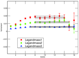
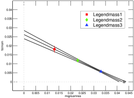
Figure 1: Left: Jack-knife results for $\langle\,\xi\,\rangle^{\textrm{bare}}$ as a function of the time. The ranges over which we fit and the corresponding results are indicated by the black lines. Right: Linear chiral extrapolation for $\langle\,\xi\,\rangle^{\textrm{bare}}$.

4.2 Chiral extrapolation

Plotting our results for $\langle\,\xi\,\rangle^{\textrm{bare}}$ as a function of the light-quark mass in the right plot in fig. 1 and taking into account the remnant chiral symmetry breaking by defining the chiral limit at the point $am_{q}+am_{\rm res}=0$ our data confirms the linear behaviour predicted by chiral perturbation theory [36, 37]. Moreover the line passes through $\langle\,\xi\,\rangle^{\textrm{bare}}=0$ at a value of the light-quark mass (denoted by the open square) which is consistent with the mass of the strange quark, as expected for the $SU(3)$ symmetric case ($am_{ud}=am_{s}=0.04$). From the linear fit we obtain $\langle\,\xi\,\rangle^{\textrm{bare}}=0.0262(23)$ in the chiral limit.

5 Systematic Uncertainties and our Final Result

Combining $\langle\,\xi\,\rangle^{\rm bare}$ with the result for the perturbative renormalization factor we obtain our final result

$$\langle\,\xi\,\rangle^{{\overline{\mathrm{MS}}}}(\mu=1.6\,\textrm{GeV})=0.034\pm 0.003\,.$$ (13)

In order to compare our result with previous calculations we evolve it to the renormalization scales 1 GeV and 2 GeV using the three-loop anomalous dimension [38]. We obtain $\langle\,\xi\,\rangle^{{\overline{\mathrm{MS}}}}(\mu=2\,\textrm{GeV})=0.032\pm 0.003$ and $\langle\,\xi\,\rangle^{{\overline{\mathrm{MS}}}}(\mu=1\,\textrm{GeV})=0.040\pm 0.004$.
The error in the renormalization factor due to the uncertainty in the lattice spacing is negligible. For example if we conservatively allow the lattice spacing to vary between 1.58 GeV and 1.62 GeV, the contribution to the relative error on $\langle\,\xi\,\rangle^{{\overline{\mathrm{MS}}}}$ is less than 0.2%.

Among the uncertainties which we are not at this stage in a position to check numerically are the continuum extrapolation, finite-volume effects and the fact that the strange quark mass ($m_{s}a=0.04$) is only approximately tuned to its physical value. The lattice artefacts are formally of $O(a^{2}\Lambda^{2}_{\textrm{Q}CD})\simeq 2.5\%$ and we are planning to check this with a simulation at a smaller lattice spacing. We would expect the finite volume effects to be small and are currently checking this with a simulation on a $24^{3}\times 64$ lattice. The strange quark mass appears to be well tuned [22, 23] so again we expect the contribution to the error from this uncertainty to be very small. Thus we expect the errors from these three sources to be sufficiently small not to change the errors quoted for our final result. We are also carrying out a systematic programme of non-perturbative renormalization which will enable us to reduce the uncertainty in the renormalization constants.

6 Summary and Conclusions

We have demonstrated that the $SU(3)$-breaking effects which lead to a non-zero value for the first moment of the kaon’s distribution amplitude are sufficiently large to be calculable in lattice simulations and satisfy the expected chiral behaviour. As our best result we quote $\langle\,\xi\,\rangle^{{\overline{\mathrm{MS}}}}(\mu=1.6\,\textrm{GeV})=0.034\pm 0.003$.
Acknowledgements

The development and computer equipment used in this calculation were funded by the U.S. DOE grant DE-FG02-92ER40699, PPARC JIF grant PPA/J/S/1998/00756 and by RIKEN. This work was supported by PPARC grants PPA/G/O/2002/00465, PPA/G/S/2002/00467 and PP/D000211/1. JN acknowledges support from the Japanese Society for the Promotion of Science.

References

- [1] UKQCD Collaboration, P.A. Boyle et al., Phys. Lett. B641 (2006) 67, hep-lat/0607018.
- [2] V.L. Chernyak and A.R. Zhitnitsky, JETP Lett. 25 (1977) 510.
- [3] V.L. Chernyak and A.R. Zhitnitsky, Sov. J. Nucl. Phys. 31 (1980) 544.
- [4] A.V. Efremov and A.V. Radyushkin, Phys. Lett. B94 (1980) 245.
- [5] A.V. Efremov and A.V. Radyushkin, Theor. Math. Phys. 42 (1980) 97.
- [6] V.L. Chernyak, A.R. Zhitnitsky and V.G. Serbo, JETP Lett. 26 (1977) 594.
- [7] V.L. Chernyak, V.G. Serbo and A.R. Zhitnitsky, Sov. J. Nucl. Phys. 31 (1980) 552.
- [8] G.P. Lepage and S.J. Brodsky, Phys. Rev. D22 (1980) 2157.
- [9] M. Beneke, G. Buchalla, M. Neubert and C.T. Sachrajda, Phys. Rev. Lett. 83 (1999) 1914, hep-ph/9905312.
- [10] M. Beneke, G. Buchalla, M. Neubert and C.T. Sachrajda, Nucl. Phys. B591 (2000) 313, hep-ph/0006124.
- [11] M. Beneke, G. Buchalla, M. Neubert and C.T. Sachrajda, Nucl. Phys. B606 (2001) 245, hep-ph/0104110.
- [12] C.W. Bauer, S. Fleming and M.E. Luke, Phys. Rev. D63 (2001) 014006, hep-ph/0005275.
- [13] C.W. Bauer, S. Fleming, D. Pirjol and I.W. Stewart, Phys. Rev. D63 (2001) 114020, hep-ph/0011336.
- [14] C.W. Bauer and I.W. Stewart, Phys. Lett. B516 (2001) 134, hep-ph/0107001.
- [15] C.W. Bauer, D. Pirjol and I.W. Stewart, Phys. Rev. D65 (2002) 054022, hep-ph/0109045.
- [16] A. Khodjamirian, T. Mannel and M. Melcher, Phys. Rev. D70 (2004) 094002, hep-ph/0407226.
- [17] V.M. Braun and A. Lenz, Phys. Rev. D70 (2004) 074020, hep-ph/0407282.
- [18] P. Ball and R. Zwicky, Phys. Lett. B633 (2006) 289, hep-ph/0510338.
- [19] P. Ball and R. Zwicky, JHEP 02 (2006) 034, hep-ph/0601086.
- [20] V.M. Braun et al. (2006), hep-lat/0606012.
- [21] UKQCD and RBC Collaborations, R. D. Mawhinney et al., in these proceedings PoS(LAT2006)188 .
- [22] UKQCD and RBC Collaborations, R. Tweedie et al., in these proceedings PoS(LAT2006)096 .
- [23] UKQCD and RBC Collaborations, paper in preparation .
- [24] D.B. Kaplan, Phys. Lett. B288 (1992) 342, hep-lat/9206013.
- [25] V. Furman and Y. Shamir, Nucl. Phys. B439 (1995) 54, hep-lat/9405004.
- [26] Y. Iwasaki and T. Yoshié, Phys. Lett. B143 (1984) 449.
- [27] Y. Iwasaki, Nucl. Phys. B258 (1985) 141.
- [28] M. Göckeler et al., Phys. Rev. D54 (1996) 5705, hep-lat/9602029.
- [29] S. Aoki, T. Izubuchi, Y. Kuramashi and Y. Taniguchi, Phys. Rev. D67 (2003) 094502, hep-lat/0206013.
- [30] S. Aoki, T. Izubuchi, Y. Kuramashi and Y. Taniguchi, Phys. Rev. D59 (1999) 094505, hep-lat/9810020.
- [31] S. Capitani, Phys. Rev. D73 (2006) 014505, hep-lat/0510091.
- [32] Y. Iwasaki, University of Tsukuba preprint UTHEP-118 (1983).
- [33] UKQCD Collaboration, C.R. Allton et al., Phys. Rev. D47 (1993) 5128, hep-lat/9303009.
- [34] M. Falcioni, M.L. Paciello, G. Parisi and B. Taglienti, Nucl. Phys. B251 (1985) 624.
- [35] APE Collaboration, M. Albanese et al., Phys. Lett. B192 (1987) 163.
- [36] J.W. Chen and I.W. Stewart, Phys. Rev. Lett. 92 (2004) 202001, hep-ph/0311285.
- [37] J.W. Chen, H.M. Tsai and K.C. Weng, Phys. Rev. D73 (2006) 054010, hep-ph/0511036.
- [38] S.A. Larin, T. van Ritbergen and J.A.M. Vermaseren, Nucl. Phys. B427 (1994) 41.