Gluon mass generation and infrared Abelian dominance in Yang-Mills theory KEK Preprint 2006-39 CHIBA-EP-162

Abstract:

The dual superconductivity is believed to be a promising mechanism for quark confinement. Indeed, what this picture is true has been confirmed in the maximal Abelian (MA) gauge. However, it is not yet confirmed in any other gauge and the MA gauge explicitly breaks color symmetry. To remedy this defect, we propose to use our compact formulation of a non-linear change of variables on a lattice. This formulation has succeeded to extract the magnetic monopole with integer-valued magnetic charge in the gauge-invariant way. In this talk, we present measurements of various correlation functions for the operators constructed from the CFN variables in SU(2) Yang-Mills theory. Some of our results reproduce previous results obtained in MA gauge, e.g., DeGrant-Toussaint monopole, infrared Abelian dominance and off-diagonal gluon mass generation. These studies preserve color symmetry, in sharp contrast to the conventional MA gauge. We argue the gauge fixing independence of these results and the implications to quark confinement.

1 Introduction

Quark confinement is still an unsolved and challenging problem in theoretical particle physics. The dual superconductivity[2] is believed to be a promising mechanism for the vacuum of the non-Abelian gauge theory[1]. Indeed, the relevant data supporting the validity of this picture have been accumulated by numerical simulations especially since 1990 and some of the theoretical predictions [3, 4] have been confirmed by these investigations: infrared Abelian dominance [5], magnetic monopole dominance [6] and non-vanishing off-diagonal gluon mass [7] in the Maximal Abelian gauge [8], which are the most characteristic features for the dual superconductivity. However, they are not yet confirmed in any other gauge and the MA gauge explicitly breaks color symmetry. To establish this picture in gauge invariant way, we need to answer how to define and extract the “Abelian part” $\mathbb{V}_{\mu}$ from the original non-Abelian gauge field $\mathcal{A}_{\mu}$ which is responsible for the area decay law of the Wilson loop average. The conventional Abelian projection [3] is too naive to realize this requirement. At the same time, we must answer why the remaining part $\mathbb{X}_{\mu}$ in the non-Abelian gauge field $\mathcal{A}_{\mu}$ decouple in the low-energy (or long-distance) regime.

We propose to use a non-linear change of variables (NLCV) which was called the Cho-Faddeev-Niemi (CFN) decomposition[11, 12, 13, 14] to remedy the defect of ordinary approaches. [15, 16, 18] We introduce a compact representation of NLCV on a lattice. The naive decomposition presented at the last conference was improved to extract the magnetic monopole with integer-valued magnetic charge in the gauge-invariant way.[19] Some of our results reproduce previous results obtained in MA gauge, e.g., DeGrant-Toussaint monopole, infrared Abelian dominance.

2 Lattice CFN variables or NLCV on a lattice

We propose a formulation of NLCV on a lattice It is a minimum requirement that such a lattice formulation must reproduce the continuum counterparts in the naive continuum limit.  In the continuum formulation [12, 10], a color vector field $\vec{n}(x)=(n_{A}(x))$ $(A=1,2,3)$ is introduced as a three-dimensional unit vector field. In what follows, we use the boldface to express the Lie-algebra $su(2)$-valued field, e.g., $\mathbf{n}(x):=n_{A}(x)T_{A}$, $T_{A}=\frac{1}{2}\sigma_{A}$ with Pauli matrices $\sigma_{A}$ ($A=1,2,3$). Then the $su(2)$-valued gluon field (gauge potential) $\mathbf{A}_{\mu}(x)$ is decomposed into two parts:

$$\mathbf{A}_{\mu}(x)=\mathbf{V}_{\mu}(x)+\mathbf{X}_{\mu}(x),$$ (1)

in such a way that the color vector field $\mathbf{n}(x)$ is covariant constant in the background field $\mathbf{V}_{\mu}(x)$:

$$0=\mathcal{D}_{\mu}[\mathbf{V}]\mathbf{n}(x):=\partial_{\mu}\mathbf{n}(x)-ig[\mathbf{V}_{\mu}(x),\mathbf{n}(x)],$$ (2)

and that the remaining field $\mathbf{X}_{\mu}(x)$ is perpendicular to $\mathbf{n}(x)$:

$$\vec{n}(x)\cdot\vec{X}_{\mu}(x)\equiv 2\mathrm{tr}(\mathbf{n}(x)\mathbf{X}_{\mu}(x))=0.$$ (3)

Here we have adopted the normalization $\mathrm{tr}(T_{A}T_{B})=\frac{1}{2}\delta_{AB}$. Both $\mathbf{n}(x)$ and $\mathbf{A}_{\mu}(x)$ are Hermitian fields. This is also the case for $\mathbf{V}_{\mu}(x)$ and $\mathbf{X}_{\mu}(x)$. By solving the defining equation (2), the $\mathbf{V}_{\mu}(x)$ and the $\mathbf{X}_{\mu}(x).$ are obtained in the form:

$$\mathbf{V}_{\mu}(x) =\mathbf{V}_{\mu}^{\parallel}(x)+\mathbf{V}_{\mu}^{\perp}(x)=c_{\mu}(x)\mathbf{n}(x)-ig^{-1}[\partial_{\mu}\mathbf{n}(x),\mathbf{n}(x)],$$ (4)

$$\mathbf{X}_{\mu}(x) =-ig^{-1}\left[\mathbf{n}(x),\mathcal{D}_{\mu}[\mathbf{A}]\mathbf{n}(x)\right]$$ (5)

where the second term $\mathbf{V}_{\mu}^{\perp}(x):=-ig^{-1}[\partial_{\mu}\mathbf{n}(x),\mathbf{n}(x)]=g^{-1}(\partial_{\mu}\vec{n}(x)\times\vec{n}(x))_{A}T_{A}$ is perpendicular to $\mathbf{n}(x)$, i.e., $\vec{n}(x)\cdot\vec{V}_{\mu}^{\perp}(x)\equiv 2\mathrm{tr}(\mathbf{n}(x)\mathbf{V}_{\mu}^{\perp}(x))=0$. Here it should be remarked that the parallel part $\mathbf{V}_{\mu}^{\parallel}(x)=c_{\mu}(x)\mathbf{n}(x)$, $c_{\mu}(x)=\mathrm{tr}(\mathbf{n}(x)\mathbf{A}_{\mu}(x))$ proportional to $\mathbf{n}(x)$ can not be determined uniquely only from the defining equation (2), and the perpendicular condition of (3) determines $\mathbf{V}_{\mu}^{\parallel}(x)$ and remainder part $\mathbf{X}_{\mu}(x).$

On a lattice, on the other hand, we introduce the site variable $\mathbf{n}_{x}=n_{x}^{A}\sigma_{A}$ in addition to the original link variable $U_{x,\mu}$ which is related to the gauge potential $\mathbb{A}_{x^{\prime},\mu}$:

$$U_{x,\mu}=\exp(-i\epsilon g\mathbb{A}_{x^{\prime},\mu},),$$ (6)

where $\left(x^{\prime},\mu\right)=(x+\mu/2,\mu)$ stand for the midpoint of the link.

In what follows, we use the blackboard boldface to express the field determined by the link variable. Note that $\mathbf{n}_{x}$ is Hermitian, $\mathbf{n}_{x}^{\dagger}=\mathbf{n}_{x}$, and $U_{x,\mu}$ is unitary, $U_{x,\mu}^{\dagger}=U_{x,\mu}^{-1}$.  The link variable $U_{x,\mu}$ and the site variable $\mathbf{n}_{x}$ transform under the gauge transformation II [10] as

$$U_{x,\mu}\rightarrow\Omega_{x}U_{x,\mu}\Omega_{x+\mu}^{\dagger}=U_{x,\mu}^{\prime},\quad\mathbf{n}_{x}\rightarrow\Omega_{x}\mathbf{n}_{x}\Omega_{x}^{\dagger}=\mathbf{n}_{x}^{\prime}.$$ (7)

Suppose we have obtained a ”link variable” $V_{x,\mu}$ and $X_{x,\mu}$ as a group element of $G=SU(2)$ through

$$V_{x,\mu} =\exp(-i\epsilon g\mathbb{V}_{x^{\prime},\mu}),$$ (8)

$$\ X_{x,\mu} =\exp(-i\epsilon g\mathbb{X}_{x,\mu}).$$ (9)

$\mathbb{V}_{x^{\prime},\mu}$are related to the $su(2)$-valued background field $\mathbb{V}_{x^{\prime},\mu}$ where $\mathbb{V}_{x^{\prime},\mu}$ is to be identified with the continuum variable (4) and hence $V_{x,\mu}$ must be unitary $V_{x,\mu}^{\dagger}=V_{x,\mu}^{-1}$. A lattice version of defining equation (2) and (3) are given by

$$D_{\mu}^{(\epsilon)}[\mathbf{V}]\mathbf{n}_{x}:=\epsilon^{-1}[V_{x,\mu}\mathbf{n}_{x+\mu}-\mathbf{n}_{x}V_{x,\mu}]=0,$$ (10)

$$\mathrm{tr}(\mathbf{n}_{x}X_{x,\mu})=0.$$ (11)

The defining equation (10) needs a lattice covariant derivative for an adjoint field. We adopt the midpoint evaluation of the difference $\partial_{\mu}^{(\epsilon)}\mathbf{n}_{x}=\epsilon^{-1}[\mathbf{n}_{x+\mu}-\mathbf{n}_{x}]=\partial_{\mu}\mathbf{n}_{x^{\prime}}+$ $\mathcal{O}(\epsilon^{2})$, therefore the continuum covariant derivative for the adjoint field up to $\mathcal{O}(\epsilon^{2})$ at midpoint:

$$\epsilon^{-1}[V_{x,\mu}\mathbf{n}_{x+\mu}-\mathbf{n}_{x}V_{x,\mu}]=\partial_{\mu}\mathbf{n}_{x^{\prime}}-ig[\mathbb{V}_{x^{\prime},\mu},\mathbf{n}_{x^{\prime}}]-\frac{i\epsilon}{2}\left\{g\mathbb{V}_{x^{\prime},\mu},\partial_{\mu}\mathbf{n}_{x^{\prime}}\right\}+\mathcal{O}(\epsilon^{2}).$$

The derivative (10) obeys the correct transformation property, i.e., the adjoint rotation on a lattice:

$$D_{\mu}^{(\epsilon)}[\mathbf{V}]\mathbf{n}_{x}\rightarrow\Omega_{x}(D_{\mu}^{(\epsilon)}[\mathbf{V}]\mathbf{n}_{x})\Omega_{x+\mu}^{\dagger},$$

provided that the link variable $V_{x,\mu}$ transforms in the same way as the original link variable $U_{x,\mu}$:

$$V_{x,\mu}\rightarrow\Omega_{x}V_{x,\mu}\Omega_{x+\mu}^{\dagger}=V_{x,\mu}^{\prime}.$$ (12)

This is required from the transformation property of the continuum variable $\mathbf{V}_{\mu}(x)$, see [10]. Therefore, we obtain the desired condition between $\mathbf{n}_{x}$ and $V_{x,\mu}$.

$$\mathbf{n}_{x}V_{x,\mu}=V_{x,\mu}\mathbf{n}_{x+\mu}.$$ (13)

The defining equation (13) for the link variable $V_{x,\mu}$ is form-invariant under the gauge transformation II, i.e., $\mathbf{n}_{x}^{\prime}V_{x,\mu}^{\prime}=V_{x,\mu}^{\prime}\mathbf{n}_{x+\mu}^{\prime}$.

A lattice version of the orthogonality equation (3) given by equation(11) or

$$\mathrm{tr}(\mathbf{n}_{x}\exp\{-i\epsilon g\mathbb{X}_{x,\mu}\})=\mathrm{tr}(\mathbf{n}_{x}\{\mathbf{1}-i\epsilon g\mathbb{X}_{x,\mu}\})+\mathcal{O}(\epsilon^{2})=0+\mathcal{O}(\epsilon^{2}).$$ (14)

This implies that the trace vanishes up to first order of $\epsilon$ apart from the second order term.  Note that $X_{x,\mu}$ is defined on the lattice site and transforms in the same way as $\mathbf{n}_{x}$:

$$X_{x,\mu}\rightarrow\Omega_{x}X_{x,\mu}\Omega_{x}^{\dagger}=X_{x,\mu}^{\prime}\,,$$ (15)

so that orthogonality condition (11) is gauge invariant.

Then, we proceed to solve the defining equation (13) for the link variable $V_{x,\mu}$ and equation (11) for the variable $X_{x,\mu},$ and express it in terms of the site variable $\mathbf{n}_{x}$ and the original link variable $U_{x,\mu}$, as is the case that the continuum variable $\mathbf{V}_{\mu}(x)$ and $\mathbf{X}_{\mu}(x)$ are expressed in terms of $\mathbf{n}(x)$ and $\mathbf{A}_{\mu}(x)$. Remembering the relation $\mathbb{X}_{x,\mu}=\mathbb{A}_{x,\mu}-\mathbb{V}_{x,\mu}$, $X_{x,\mu}$ can be defined using link variables $V_{x,\mu}$ and $U_{x,\mu}$ contacting to site $x$, and linear combination of $V_{x-\mu,\mu}^{\dagger}U_{x-\mu,\mu}$ and $U_{x,\mu}V_{x,\mu}^{\dagger},$ are candidate to satisfy the required transformation property (15);

$$X_{x,\mu} =\lambda V_{x-\mu,\mu}^{\dagger}U_{x-\mu,\mu}+\phi U_{x,\mu}V_{x,\mu}^{\dagger}$$ (16)

$$=\exp(-i\epsilon g\mathbb{X}_{x,\mu})\left[\lambda+\phi+(\lambda-\phi)\frac{g^{2}\epsilon^{2}}{2}[\mathbb{V}_{x},\mathbb{A}_{x,\mu}]+\mathcal{O}(\epsilon^{3})\right],$$

where the relation for matrices $\exp(\epsilon A)\exp(\epsilon B)=\exp(\epsilon A+\epsilon B+\epsilon^{2}[A,B]/2+\mathcal{O}(\epsilon^{3}))$ and its inverted version of $\exp(\epsilon C+\epsilon^{2}D)=\exp(\epsilon C)\exp(\epsilon^{2}D)+\mathcal{O}(\epsilon^{3})~{}$are used. The parameter $\lambda=\phi$   is selected so that $X_{x,\mu}$ is determined to coincide with continuum expression up to $\mathcal{O}(\epsilon^{3})$.

As for $V_{x,\mu}$, on the other hand, the equation (13) is a matrix equation and it is rather difficult to obtain the general solution. Therefore, we adopt an ansatz (up to quadratic in $\mathbf{n}$):

$$V_{x,\mu}=U_{x,\mu}+\alpha\mathbf{n}_{x}U_{x,\mu}+\beta U_{x,\mu}\mathbf{n}_{x+\mu}+\gamma\mathbf{n}_{x}U_{x,\mu}\mathbf{n}_{x+\mu},$$ (17)

which enjoys the correct transformation property, the adjoint rotation (12). It turns out that this ansatz satisfy the defining equation (13), if and only if the numerical coefficients $\alpha,\beta$ and $\gamma$ are chosen to be $\gamma=1$ and $\alpha=\beta.$ Then, substituting the ansatz (17) with a still undetermined parameter $\alpha$ into equation (16), we obtain $\alpha=0+\mathcal{O}(\epsilon^{2})$ (see [18]).

Thus we have determined $V_{x,\mu}$ and $X_{x,\mu}$ up to an overall normalization

$$V_{x,\mu} =V_{x,\mu}[U,\mathbf{n}]=U_{x,\mu}+\mathbf{n}_{x}U_{x,\mu}\mathbf{n}_{x+\mu}\,,$$

$$X_{x,\mu} =X_{x,\mu}[U,\mathbf{n}]=V_{x-\mu,\mu}^{\dagger}U_{x-\mu,\mu}+U_{x,\mu}V_{x,\mu}^{\dagger}\,.$$

The unitary link variable $\hat{V}_{x,\mu}[U,\mathbf{n}]$ and $\hat{X}_{x,\mu}[U,\mathbf{n}]$ can be obtained after the normalization:

$$\hat{V}_{x,\mu}[U,\mathbf{n}]:=V_{x,\mu}/\sqrt{\frac{1}{2}\mathrm{tr}[V_{x,\mu}^{\dagger}V_{x,\mu}]},\qquad\hat{X}_{x,\mu}[U,\mathbf{n}]:=X_{x,\mu}/\sqrt{\frac{1}{2}\mathrm{tr}[X_{x,\mu}^{\dagger}X_{x,\mu}]}.$$ (18)

3 Numerical simulations and generation of configuration of NLCV

We generate configurations of link variables $\{U_{x,\mu}\}$ using standard Wilson action. The numerical simulation are performed on $24^{4}$ lattice at $\beta=2.3$, $2.4$, $2.5$ by thermalizing 15000 sweeps, and on $36^{4}$ lattice at $\beta=2.5$, $2.6$, $2.7$ by thermalizing 18000 sweeps. 200 configurations are obtained every 300 sweeps.

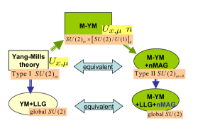
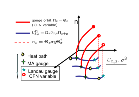
Figure 1: (left)The relationship between the master-YM theory and the original YM theory. (right) NLCV via gauge transfroamtion.

The NLCV on a lattice is obtained according to the method of the previous paper [18]. Figure 1 shows the extended gauge symmetry in the master-YM for NLCV (left panel) and NLCV of SU(2) link variables via gauge transformations (right panel).  The configuration of  the link variable $U_{x,\mu}$ and the color vector field $\mathbf{n}_{x}$ has an extended gauge symmetry $SU(2)_{\omega}\times\left[SU(2)/U(1)\right]_{\theta}$. The equivalent theory to the original YM theory is obtained by the gauge fixing which we call the new Maximal Abelian gauge (nMAG). We define a functional written in terms of the gauge (link) variable $U_{x,\mu}$ and the color (site) variable $\mathbf{n}_{x}$; $F_{nMAG}[U,\mathbf{n};\Omega,\Theta]\equiv\sum_{x,\mu}\mathrm{tr}(\mathbf{1}-{}^{\Theta}\mathbf{n}_{x}{}^{\Omega}U_{x,\mu}{}^{\Theta}\mathbf{n}_{x+\mu}{}^{\Omega}U_{x,\mu}^{\dagger})$, where we have introduced the enlarged gauge transformation: ${}^{\Omega}{}U_{x,\mu}:=\Omega_{x}U_{x,\mu}\Omega_{x+\mu}^{\dagger}$ for the link variable $U_{x,\mu}$ and ${}^{\Theta}\mathbf{n}_{x}:=\Theta_{x}\mathbf{n}_{x}^{(0)}\Theta_{x}^{\dagger}$ for an initial site variable $\mathbf{n}_{x}^{(0)}$. The gauge group elements $\Omega_{x}$ and $\Theta_{x}$ are independent SU(2) matrices on a site $x$. After imposing the nMAG, the theory still has the local gauge symmetry $SU(2)_{local}^{\omega=\theta}$, since the “diagonal” gauge transformation $\mathbf{\omega}=\mathbf{\theta}$ does not change the value of the functional $F_{nMAG}[U,\mathbf{n};\Omega,\Theta]$. Therefore, the configuration of $\mathbf{n}_{x}$ can not be determined at this stage. In order to determine $\mathbf{n}_{x}$, we need to impose another gauge fixing or a choice of the gauge of link variable $U_{x,\mu}$ for fixing $SU(2)_{\omega}$. The desired color vector field $\mathbf{n}_{x}$ is constructed from the interpolating gauge transformation matrix $\Theta_{x}$ by choosing the initial value $\mathbf{n}_{x}^{(0)}=\sigma_{3}$ and $\mathbf{n}_{x}:=\Theta_{x}\sigma_{3}\Theta_{x}^{\dagger}=n_{x}^{A}\sigma^{A}$, $n_{x}^{A}=\mathrm{tr}[\sigma_{A}\Theta_{x}\sigma_{3}\Theta_{x}^{\dagger}]/2$ ($A=1,2,3$) where $\left\{\Theta_{x}\right\}$ are given by gauge transformations that satisfy $U_{x,\mu}=\Theta_{x}U_{x,\mu}^{MAG}\Theta_{x+\mu}^{\dagger}.$ For example, we choose the conventional Lorentz-Landau gauge or Lattice Landau gauge (LLG) for this purpose. The LLG can be imposed by minimizing the function $F_{LLG}[U;\Omega]=\sum_{x,\mu}\mathrm{tr}(\mathbf{1}-{}^{\Omega}U_{x,\mu})$ with respect to the gauge transformation $\Omega_{x}$ for the given link configurations $\{U_{x,\mu}\}$.

4 Infrared Abelian Dominance and Mass generation of the off-diagonal gluon

Using new variables through NLCV,  we are now ready to study characteristic features of the YM theory for any choice of gauge fixing such as infrared Abelian dominance, magnetic monopole dominance and the non-vanishing off-diagonal gluon mass. Our proposed decomposition extract the “Abelian part” $V_{x,\mu}$ in any gauge fixing preserving the color symmetry. The conventional MAG fixed theory is reproduced as a special case of  our formulation base on NLCV. To study the infrared Abelian dominance and the non-vanishing off-diagonal gluon mass in LLG other than MAG, the correlation function of the decomposed variable $V_{x,\mu}$ and $X_{x,\mu}$ has been measured. Left panel of figure 2 shows propagators $D_{AA}(x-y)=\left\langle\mathbb{A}_{x,\mu}\mathbb{A}_{y,\mu}\right\rangle$, $D_{VV}(x-y)=\left\langle\mathbb{V}_{x,\mu}\mathbb{V}_{y,\mu}\right\rangle$ and $D_{XX}(x-y)=\left\langle\mathbb{X}_{x,\mu}\mathbb{X}_{y,\mu}\right\rangle$. The gauge potentials are defined as link variables $\mathbb{A}_{x^{\prime},\mu}=\frac{-i}{2g\varepsilon}\left[A_{x,\mu}-A_{x,\mu}^{\dagger}\right]$, $\mathbb{V}_{x^{\prime},\mu}=\frac{-i}{2g\varepsilon}\left[V_{x,\mu}-V_{x,\mu}^{\dagger}\right].$ On the other hand, we can define the $\mathbb{X}_{x,\mu}$ in two ways, one is extracted from compact representation, $\mathbb{X}_{x,\mu}=\frac{-i}{2g\varepsilon}\left[X_{x,\mu}-X_{x,\mu}^{\dagger}\right],$ and the other is from definition of the decomposition (1), $\mathbb{X}_{x^{\prime},\mu}=\mathbb{A}_{x^{\prime},\mu}-\mathbb{V}_{x^{\prime},\mu}.$ Plotting of two types of $D_{XX}(x-y)$ overlap for several lattice spacings (several $\beta$s) , and the extracttion of the variable is consistent (see left panel of figure 2). On the other hand, $D_{AA}(x-y)$ and $D_{VV}(x-y)$ overlap, and $D_{XX}(x-y)$ is dumped more quickly for infrared region than $D_{VV}(x-y)$. This implies that the infrared Abelian dominance is found in the LLG.

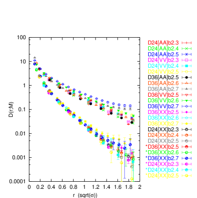
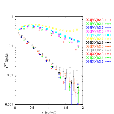
Figure 2: (left) correlation functions$\left\langle O(x)O(y)\right\rangle$ in the logalithmic scale, (right) rescaled correratin function $\ln\left(r^{3/2}G_{\mu\mu}(r;M)\right)$

Next we study the mass of the decomposed fields from the correlation functions.  The inverse Fourier transformation of the massive gauge boson propagator should behave for large $r=|x-y|$ as follows,

$$G_{\mu\mu}(r;M)=\left\langle\mathbb{X}_{\mu}(x)\mathbb{X}_{\mu}(y)\right\rangle=\int\frac{d^{4}k}{(2\pi)^{4}}e^{ik(x-y)}\frac{1}{k^{2}+M^{2}}\left(4+\frac{k^{2}}{M^{2}}\right)\simeq\frac{3\sqrt{M}}{2(2\pi)^{3/2}}\frac{e^{-Mr}}{r^{3/2}}\,.$$

So the scaled propagator $r^{3/2}G_{\mu\mu}(r;M)$ is proportional to $e^{-Mr}$, that is, the mass of gauge potential $M$, is obtained as the dumping factor of $r^{3/2}G_{\mu\mu}(r;M)$. In other words, the gradient of the linear fitting in the $r$ vs $\ln\left(r^{3/2}G_{\mu\mu}(r;M)\right)$ plot gives the mass   $M$.  Right panel of figure 2 shows the plots of the scaled propagator of $\ \mathbb{X}_{x^{\prime},\mu}$ and $\mathbb{V}_{x^{\prime},\mu}$. The distance $r$ is measured in the unit of square root of the string tension $\sqrt{\sigma_{ST}}$ ($=440$ MeV), and vertical axis is scaled in the logarithm to measure the dumping factor by the linear fitting. To determine the physical scale, the relation between $\beta$ and lattice spacing $\epsilon$ is obtained from [21]. The dumping of propagator of $\mathbb{X}_{x,\mu}\,$ gives the mass $M_{X}\simeq 1.18$ GeV, and the “Abelian part” $\mathbb{V}_{x,\mu}$ indicates $M_{V}\simeq 0.48$ GeV. These are consistent with study in MAG.[7]

5 Summary and discussion

We have proposed a new formulation of  the lattice Yang-Mills theory based on the NLCV which was once called the CFN decomposition. This resolves all drawbacks of the previous formulation of the decomposition on a lattice. This compact formulation enables us to guarantee the magnetic charge quantization in the gauge invariant way and to extract the “Abelian part” and the “off-diagonal part” preserving color symmetry  in any choice of gauge of the original YM theory. These features are sharp contrast to the conventional MA gauge and these studies. We have measured the correlation function (propagator in real space) in LLG. The Infrared Abelian dominance and the gluon mass generation have been found. These results are consistent with study in MA gauge.

References

• [1] C.N. Yang and R.L. Mills, Phys. Rev. 96, 191-195 (1954); R. Utiyama, Phys. Rev. 101, 1597-1607 (1956).
• [2] Y. Nambu, Phys. Rev. D 10, 4262 (1974); G. ’t Hooft, in: High Energy Physics, edited by A. Zichichi (Editorice Compositori, Bologna, 1975); S. Mandelstam, Phys. Report 23, 245 (1976); A.M. Polyakov, (1975). Nucl. Phys. B 120, 429 (1977).
• [3] G. ’t Hooft, Nucl.Phys. B190 [FS3], 455 (1981).
• [4] Z.F. Ezawa and A. Iwazaki, Phys. Rev. D25, 2681 (1982).
• [5] T. Suzuki and I. Yotsuyanagi, Phys. Rev. D42, 4257 (1990).
• [6] J.D. Stack, S.D. Neiman and R. Wensley, [hep-lat/9404014], Phys. Rev. D50, 3399 (1994); H. Shiba and T. Suzuki, Phys.Lett.B333, 461 (1994).
• [7] K. Amemiya and H. Suganuma, [hep-lat/9811035], Phys. Rev. D60, 114509 (1999); V.G. Bornyakov, M.N. Chernodub, F.V. Gubarev, S.M. Morozov and M.I. Polikarpov,[hep-lat/0302002], Phys. Lett. B559, 214-222 (2003).
• [8] A. Kronfeld, M. Laursen, G. Schierholz and U.-J. Wiese, Phys.Lett. B 198, 516 (1987).
• [9] F.V. Gubarev, L. Stodolsky and V.I. Zakharov, [hep-ph/0010057], Phys. Rev. Lett. 86, 2220–2222 (2001).; F.V. Gubarev and V.I. Zakharov, [hep-ph/0010096], Phys. Lett. B 501, 28–36 (2001).
• [10] K.-I. Kondo, T. Murakami and T. Shinohara, [hep-th/0504107], Prog. Theor. Phys. 115, 201 (2006). K.-I. Kondo, T. Murakami and T. Shinohara, [hep-th/0504198], Eur. Phys. J. C 42, 475 (2005).
• [11] Y.S. Duan and M.L. Ge, Sinica Sci., 11, 1072 (1979).
• [12] Y.M. Cho, Phys. Rev. D 21, 1080 (1980). Phys. Rev. D 23, 2415 (1981).
• [13] L. Faddeev and A.J. Niemi, [hep-th/9807069], Phys. Rev. Lett. 82, 1624 (1999).
• [14] S.V. Shabanov, [hep-th/9903223], Phys. Lett. B 458, 322 (1999). S.V. Shabanov, [hep-th/9907182], Phys. Lett. B 463, 263 (1999).
• [15] S. Kato, K.-I. Kondo, T. Murakami, A. Shibata and T. Shinohara, hep-ph/0504054.
• [16] A.Shibata S. Kato, S.Ito, K.-I. Kondo, T. Murakami, A. Shibata and T. Shinohara, [hep-lat/0510027], PoS LAT2005:332,2006
• [17] K.-I. Kondo, T. Murakami and T. Shinohara, [hep-th/0504107], Prog. Theor. Phys. 115, 201 (2006). K.-I. Kondo, T. Murakami and T. Shinohara, [hep-th/0504198], Eur. Phys. J. C 42, 475 (2005).
• [18] S. Kato, K.-I. Kondo, T. Murakami, A. Shibata, T. Shinohara and S. Ito, [hep-lat/0509069], Phys. Lett. B 632, 326–332 (2006).
• [19] S. Ito, S. Kato, K.-I. Kondo, T. Murakami, A. Shibata and T. Shinohara, [hep-lat/0604016].
• [20] S. Kato, S.Ito, K.-I. Kondo, T. Murakami, A. Shibata and T. Shinohara, A talk in Lattice2006, to appear in the Proceedings of Lattice2006, PoS Lattice(2006)068
• [21] S. Kato, S. Kitahara, N. Nakamura and T. Suzuki, Nucl. Phys. B 520, 323-344 (1998).