$m_{\rm b}$ and $f_{\rm B_{s}}$ from a combination of HQET and QCD

Abstract:

We compute the mass of the b-quark and the $\mathrm{B_{s}}$ meson decay constant in quenched lattice QCD using a combination of HQET and the standard relativistic QCD Lagrangian. We start from a small volume, where one can directly deal with the b-quark, and compute the evolution to a big volume, where the finite size effects are negligible through step scaling functions which give the change of the observables when $L$ is changed to $2L$. In all steps we extrapolate to the continuum limit, separately in HQET and in QCD for masses below $m_{\mathrm{b}}$. The point $m_{\mathrm{b}}$ is then reached by an interpolation of the continuum results. With $r_{0}=0.5\,{\rm fm}$ and the experimental $B_{\mathrm{s}}$ and $K$ masses we find $f_{\rm B_{\rm s}}=191(6)$ MeV and the renormalization group invariant mass $M_{\mathrm{b}}=6.89(11)$ GeV, translating into $\kern 1.0pt\overline{\kern-1.0ptm\kern-1.0pt}\kern 1.0pt_{\mathrm{b}}(\kern 1.0pt\overline{\kern-1.0ptm\kern-1.0pt}\kern 1.0pt_{\mathrm{b}})=4.42(7)$ GeV in the ${\rm\overline{MS\kern-0.50003pt}\kern 0.50003pt}$ scheme.
DESY 06-174
SFB/CPP-06-47

1 Introduction

The b-quark mass is a fundamental parameter of QCD, and its accurate knowledge is needed for theoretical predictions of B meson decay rates. The understanding of the latter is a very active field of high energy physics research. At the same time the B meson decay constant plays a crucial role in the description of these phenomena.

We focus our attention on the pseudoscalar $\mathrm{B_{s}}$ meson, a system characterized by two different scales: the heavy quark mass ($m_{\rm b}\sim 5$ GeV) and the typical QCD scale. The mass of the strange quark is around or below the latter. We fix it to its physical value through $m_{\rm K}$ as in [1].

2 HQET and step scaling method (SSM)

We deal with these two scales in (quenched) lattice QCD with the SSM introduced in [2, 3], but constraining the large mass behaviour by HQET [4]. The computation of an observable $O(m_{\rm h})$ using the SSM is based on the identity

$$O(m_{\rm h},L_{\infty})=O(m_{\rm h},L_{0})\,\hbox{$\displaystyle O(m_{\rm h},L_{1})\over\displaystyle O(m_{\rm h},L_{0})$}\,\cdots\,\hbox{$\displaystyle O(m_{\rm h},L_{N})\over\displaystyle O(m_{\rm h},L_{N-1})$}\,\hbox{$\displaystyle O(m_{\rm h},L_{\infty})\over\displaystyle O(m_{\rm h},L_{N})$}\,,$$ (1)

where $m_{\rm h}$ stands generically for a heavy quark mass whose precise definition is needed only later. In order to be able to extract each factor in the continuum limit, the starting volume $L_{0}$ has to be small enough to properly account for the dynamics of the b-quark, using a relativistic ${\rm O}(a)$-improved action. A good choice is $L_{0}=0.4$ fm  [2, 3], where easily lattice spacings of $a\approx 0.012$ fm can be used. (Physical units are set using $r_{0}=0.5$ fm  [5, 6, 7]). Furthermore, $L_{\infty}$ has to be large enough such that finite size effects in $O(m_{\rm h},L_{\infty})$ are negligible. In practise we will use $L_{\infty}\approx L_{2}=1.6$ fm. We will choose a fixed ratio $s=L_{i}/L_{i-1}$ in the step scaling functions

$$\sigma_{O}(m_{\rm h},L_{i})=\hbox{$\displaystyle O(m_{\rm h},L_{i})\over\displaystyle O(m_{\rm h},L_{i-1})$}\,.$$ (2)

The number $N$ and the scale ratio $s$ of the steps are in principle dependent on the considered observable and on the desired level of accuracy. It has been seen  [2, 3] that $(N,s)=(2,2)$ is a suitable choice for the mass and decay constant of the ${\rm B_{s}}$ meson.

In HQET the step scaling functions are expanded as

$$\sigma_{O}(m_{\rm h},L_{i})=\sigma_{O}^{(0)}(L_{i})+\hbox{$\displaystyle\sigma_{O}^{(1)}(L_{i})\over\displaystyle L_{i}m_{\rm h}$}+{\rm O}\left(\hbox{$\displaystyle 1\over\displaystyle\left(L_{i}m_{\rm h}\right)^{2}$}\right)\,$$ (3)

at fixed $L_{i}$. We will see that the correction terms to the leading order are small for the masses of interest.
We first consider the case of a finite volume pseudoscalar meson mass, $O(m_{\rm h},L)=M_{\rm PS}(m_{\rm h},L)$, which will be defined in the following section. In this case, $\sigma_{O}^{(0)}=1$ and the first non-trivial term $\sigma_{O}^{(1)}$ is computable in the static approximation of HQET. We further define

$$x(m_{\rm h},L)\equiv\hbox{$\displaystyle 1\over\displaystyle LM_{\rm PS}(m_{\rm h},L)$}=\hbox{$\displaystyle 1\over\displaystyle Lm_{\rm h}$}+{\rm O}\left(\hbox{$\displaystyle 1\over\displaystyle\left(Lm_{\rm h}\right)^{2}$}\right)\,,$$ (4)

as the natural non-perturbative dimensionless mass variable. The step scaling function for the meson mass is then written as

$$\sigma_{\rm m}(x,L_{i})\equiv\hbox{$\displaystyle M_{\rm PS}(m_{\rm h},L_{i})\over\displaystyle M_{\rm PS}(m_{\rm h},L_{i-1})$}=1+\sigma_{\rm m}^{\rm stat}(L_{i})\cdot x+{\rm O}(x^{2})\,,\quad x=x(m_{\rm h},L_{i})\,.$$ (5)

It is defined for all $x,L$. The idea for its numerical evaluation is to compute $\sigma_{\rm m}^{\rm stat}(L)$ explicitly in the static approximation and fix the small remainder by the relativistic QCD data with quarks of masses of the physical charm quark and higher. In other words we interpolate to the physical b-quark mas. With the experimental mass of the $\mathrm{B_{s}}$ meson, $M_{\rm B_{\rm s}}=5.3675(18)\,{\rm GeV}$ we fix $x_{2}=1/L_{2}M_{\rm B_{\rm s}}$ and the physical points corresponding to the b-quark are then given by

$$x_{2}=1/(L_{2}M_{\rm B_{\rm s}})\,,\quad x_{i-1}=2\sigma_{\rm m}(x_{i},L_{i})\cdot x_{i}\,.$$ (6)

The numerical results will have to be evaluated at these points. In the smallest volume we relate the meson mass to the renormalization group invariant (RGI) quark mass, $M_{\rm h}$, defining

$$\rho(x,L_{0})\equiv\hbox{$\displaystyle M_{\rm PS}(m_{\rm h},L_{0})\over\displaystyle M_{\rm h}$}=\rho^{(0)}(L_{0})+\rho^{(1)}(L_{0})\cdot x+{\rm O}(x^{2})\,.$$ (7)

We thus have the connection of the $\mathrm{B_{s}}$ meson mass and the RGI b-quark mass

$$M_{\rm b}=\hbox{$\displaystyle M_{\rm B_{\rm s}}\over\displaystyle\rho(x,L_{0})\cdot\sigma_{\rm m}(x_{1},L_{1})\cdot\sigma_{\rm m}(x_{2},L_{2})$}\,.$$ (8)

For the decay constant the step scaling function

$$\sigma_{\rm f}(x,L_{i}) \equiv \hbox{$\displaystyle f_{\rm PS}(m_{\rm h},L_{i})\sqrt{M_{\rm PS}(m_{\rm h},L_{i})}\over\displaystyle f_{\rm PS}(m_{\rm h},L_{i-1})\sqrt{M_{\rm PS}(m_{\rm h},L_{i-1})}$}=\sigma_{\rm f}^{\rm stat}(L_{i})+\sigma_{\rm f}^{(1)}(L_{i})\cdot x+{\rm O}(x^{2})\,$$ (9)

yields straightforwardly the connection between the finite volume decay constant and the infinite volume one. Note that the only approximation made in the above equations is to neglect finite size effects on mass and decay constant in the volume of linear extent $L_{2}$.

3 Finite volume observables

3.1 Relativistic QCD

Suitable finite volume observables are defined in the QCD Schrödinger functional  [8, 9] with a space-time topology $L^{3}\times T$, where $T=2L$ and $C=C^{\prime}=0$ is chosen for the boundary gauge fields, and $\theta=0$ for the phase in the spatial quark boundary conditions.
The O(a)-improved correlation functions $f_{\rm A}(m_{\rm h},L,x_{0}),f_{\rm P}(m_{\rm h},L,x_{0})$ and $f_{1}(m_{\rm h},L)$ are defined and renormalized as in  [2], allowing to compute the pseudoscalar meson decay constant

$$f_{\rm PS}(m_{\rm h},L)=\hbox{$\displaystyle-2\over\displaystyle\sqrt{L^{3}M_{\rm PS}(m_{\rm h},L)}$}\hbox{$\displaystyle f_{\rm A}(m_{\rm h},L,L)\over\displaystyle\sqrt{f_{1}(m_{\rm h},L)}$}\stackrel{{\scriptstyle m_{\rm h}\to m_{\rm b}}}{{=}}f_{\rm B_{\rm s}}(L)\stackrel{{\scriptstyle L\to\infty}}{{=}}f_{\rm B_{\rm s}}$$ (10)

and the pseudoscalar meson mass

$$M_{\rm PS}(m_{\rm h},L)=\hbox{$\displaystyle 1\over\displaystyle 2a$}\ln{\left[\hbox{$\displaystyle f_{\rm A}(m_{\rm h},L,L-a)\over\displaystyle f_{\rm A}(m_{\rm h},L,L+a)$}\right]}\stackrel{{\scriptstyle m_{\rm h}\to m_{\rm b}}}{{=}}M_{\rm B_{\rm s}}(L)\stackrel{{\scriptstyle L\to\infty}}{{=}}M_{\rm B_{\rm s}}$$ (11)

For all observables computed in relativistic (quenched) QCD we employ the non-perturbatively O(a)-improved Wilson action[10, 11]. The data at finite heavy quark mass were published in  [2, 3]. They have been reanalyzed, taking into account the correlation between observables computed on the same gauge configurations. The statistical uncertainties on the renormalization constants and the lattice spacing are included before performing the continuum limit extrapolations; they do not appear as a separate uncertainty.

3.2 HQET

In the static approximation of HQET, unrenormalized correlation functions $f_{\rm A}^{\rm stat}$ and $f_{1}^{\rm stat}$ are defined in complete analogy to the relativistic ones, see [12]. As in this reference, we use the RGI static axial current, related to the bare one by a factor $Z_{\rm RGI}$. It serves to define the RGI ratio ,

$$Y_{\rm RGI}(L)=Z_{\rm RGI}\hbox{$\displaystyle f_{\rm A}^{\rm stat}(L,L)\over\displaystyle\sqrt{f_{1}^{\rm stat}(L)}$}\,,$$ (12)

which is related to the QCD decay constant $f_{\rm PS}$ via

$$f_{\rm PS}(m_{\rm h},L)\sqrt{L^{3}M_{\rm PS}(L)}=-2C_{\rm PS}(\Lambda_{\rm\overline{MS\kern-0.35002pt}\kern 0.35002pt}/M_{\rm h})\times Y_{\rm RGI}(L)+{\rm O}(1/m_{\rm h})\,.$$ (13)

The function $C_{\rm PS}(\Lambda_{\rm\overline{MS\kern-0.35002pt}\kern 0.35002pt}/M_{\rm h})$, defined in [12], can be accurately evaluated in perturbation theory; we use the 3-loop anomalous dimension $\gamma^{\rm PS}$ computed in [13]. Just like $Z_{\rm RGI}$, it is needed only for $f_{\rm PS}(m_{\rm h},L_{0})$; it cancels out in the step scaling functions.

In analogy to eq. (11) we further define $\Gamma_{\rm stat}(L)=\hbox{$1\over 2a$}\ln\left[{f_{\rm A}^{\rm stat}(L,L-a)}/{f_{\rm A}^{\rm stat}(L,L+a)}\right]\,.$ The static step scaling functions then read

$$\sigma_{\rm f}^{\rm stat}(L_{i})=\hbox{$\displaystyle 1\over\displaystyle 2^{3/2}$}\hbox{$\displaystyle Y_{\rm RGI}(L_{i})\over\displaystyle Y_{\rm RGI}(L_{i-1})$},\quad\sigma_{\rm m}^{\rm stat}(L_{i})=L_{i}\,[\Gamma_{\rm stat}(L_{i})-\Gamma_{\rm stat}(L_{i-1})]\,,\quad L_{i}=2L_{i-1}\,.$$ (14)

These quantities will be precisely computed by using the static action denoted by HYP2 in [14] (see also [15]), and the corresponding ${\rm O}(a)$-improvement coefficients for the static axial current. The regularization independent part of the factor $Z_{\rm RGI}$ is known from [12], while the regularization dependent one is computed in this work.

4 Numerical results for the $\mathbf{b}$ quark mass

The computation of $\sigma_{\rm m}(x,L_{2})$ is performed at finite quark mass on lattices with $\beta=5.960$, $6.211,\ 6.420\$ and resolutions $L_{2}/a=16,\ 24,\ 32$; the continuum limits for the three heaviest quark masses are shown on the left of Figure 1. For the static step scaling function we took the results for $L=L_{2}$ from an extension[16] of the work of the ALPHA collaboration[17], while in the intermediate volume ($L_{1}$) we simulated lattices with $5.960\leq\beta\leq 6.737$. The continuum limit

$$\sigma_{\rm m}^{\rm stat}(L_{2})=1.549(33)\,,$$ (15)

is used in the interpolation of $\sigma_{\rm m}(x,L_{2})$ between values of $x$ corresponding to about the mass of the charm quark and the limit $\sigma_{\rm m}(0,L_{2})=1$. It constrains the slope of the fitting curve to the cone shown in Figure 1. The result of the quadratic fit in $x$ reads

$$\sigma_{\rm m}(x_{2},L_{2})=1.0328(11)\,,$$ (16)

hardly distinguishable from a purely static result. Analogously the interpolation of the step scaling function for the intermediate volume gives

$$\sigma_{\rm m}(x_{1},L_{1})=1.0092(18)\,.$$ (17)

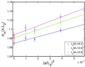
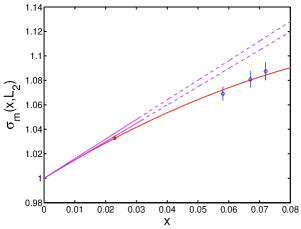
Figure 1: Continuum limit extrapolation and interpolation of $\sigma_{\mathrm{m}}(x,L_{2})$

In the small volume only the relativistic data are needed to establish a finite volume relationship between the meson and the heavy quark masses. The renormalization is non-perturbatively achieved through the renormalization factor $Z_{\rm M}(g_{0})$ and the ${\rm O}(a)$-improvement terms computed in [18, 19, 20]. Using eq. (8), the interpolated value

$$\rho(x_{0},L_{0})=0.748(11)\,,$$ (18)

is combined with the above step scaling functions to find the scale and scheme independent number

$$M_{\rm b}=6.888(105)\,{\rm GeV}\hskip 8.5359pt\Rightarrow\hskip 8.5359ptm_{{\rm b},\overline{\rm MS}}(m_{{\rm b},\overline{\rm MS}})=4.421(67)\,{\rm GeV}.$$ (19)

5 Numerical results for the decay constant

For the computation of $\sigma_{\rm f}(x,L_{2})$ the relativistic data originate from the same gauge configurations used earlier, while in the static case the decay constant in the bigger volume,

$$Y_{\rm RGI}(L_{2})=-4.63(19)\,,$$ (20)

was again computed and extrapolated to the continuum limit as an extension [16] of [17]. The continuum extrapolation of the same quantity in the intermediate volume ($L=L_{1}$) is shown on the left of Figure 2. The result

$$Y_{\rm RGI}(L_{1})=-1.628(19)$$ (21)

is used together with (20) and the relativistic data, as shown on Figure 2 (right), to get

$$\sigma_{\rm f}^{\rm stat}(L_{2})=1.006(44),\hskip 28.45274pt\sigma_{\rm f}(x_{2},L_{2})=0.974(30)\,.$$ (22)

Similarly, but by extrapolating the step scaling function to the continuum limit rather than $Y_{\rm RGI}(L_{1})$ and $Y_{\rm RGI}(L_{0})$ separately, we obtain

$$\sigma_{\rm f}^{\rm stat}(L_{1})=0.4337(44),\hskip 28.45274pt\sigma_{\rm f}(x_{1},L_{1})=0.4260(31)\,.$$ (23)

With the small volume results (see Figure 3)

$$Y_{\rm RGI}(L_{0})=-1.347(13),\hskip 28.45274ptY_{\rm PS}(x_{0},L_{0})=\hbox{$\displaystyle-f_{\rm B_{\rm s}}(L_{0})\sqrt{L_{0}^{3}M_{\rm PS}(L_{0})}\over\displaystyle 2C_{\rm PS}(\Lambda_{\rm\overline{MS\kern-0.35002pt}\kern 0.35002pt}/M_{\rm b})$}=-1.280(17)\,,$$ (24)

we finally arrive at the result

$$f_{\rm B_{\rm s}}=191(6)\,{\rm MeV}\,.$$ (25)

6 Conclusions

The combination of the Tor Vergata strategy to compute properties of heavy-light mesons  [2, 3] with the expansion of all quantities in HQET [4], changes extrapolations in the former computations into interpolations. As expected, our numerical results demonstrate that these are very well behaved. Indeed the higher order mass dependence of the step scaling functions is very weak, and in all but one steps the static approximation alone gives very accurate results. In the one exception ($Y_{\rm PS}(x_{0},L_{0})$, Fig. 3) the ${\rm O}(1/m_{{\rm b}})$ corrections are around 5%.

Our results do not suffer from any systematic errors apart from the use of the quenched approximation; small systematic errors quoted in  [2, 3] for the extrapolation uncertainties have been eliminated. Our results are in agreement with the ones of  [2, 3, 17, 21], within the errors.
Concerning dynamical fermion computations, the challenge in this strategy is to simulate in a large volume (such as $L_{2}$) with small enough lattice spacings, where quark masses of around $m_{\rm charm}$ and higher can be simulated with confidence.

Acknowledgement. We thank Michele Della Morte, Stephan Dürr, Jochen Heitger and Andreas Jüttner for useful discussions and the permission to use results of [16] prior to publication.

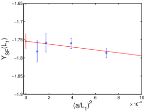
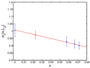
Figure 2: Continuum extrapolation of $Y_{\rm SF}(L_{1})$ and interpolation of $\sigma_{\mathrm{f}}(x,L_{2})$

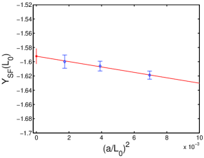
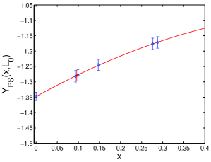
Figure 3: Continuum extrapolation of $Y_{\rm SF}(L_{0})$ and interpolation of the decay constant on the small volume

References

- [1] ALPHA, J. Garden, J. Heitger, R. Sommer and H. Wittig, Nucl. Phys. B571 (2000) 237, hep-lat/9906013.
- [2] G.M. de Divitiis, M. Guagnelli, R. Petronzio, N. Tantalo and F. Palombi, Nucl. Phys. B675 (2003) 309, hep-lat/0305018.
- [3] G.M. de Divitiis, M. Guagnelli, F. Palombi, R. Petronzio and N. Tantalo, Nucl. Phys. B672 (2003) 372, hep-lat/0307005.
- [4] ALPHA, J. Heitger and R. Sommer, JHEP 02 (2004) 022, hep-lat/0310035.
- [5] R. Sommer, Nucl. Phys. B411 (1994) 839, hep-lat/9310022.
- [6] S. Necco and R. Sommer, Phys. Lett. B523 (2001) 135, hep-ph/0109093.
- [7] M. Guagnelli, R. Petronzio and N. Tantalo, Phys. Lett. B548 (2002) 58, hep-lat/0209112.
- [8] M. Lüscher, R. Narayanan, P. Weisz and U. Wolff, Nucl. Phys. B384 (1992) 168, hep-lat/9207009.
- [9] S. Sint, Nucl. Phys. B421 (1994) 135, hep-lat/9312079.
- [10] M. Lüscher, S. Sint, R. Sommer and P. Weisz, Nucl. Phys. B478 (1996) 365, hep-lat/9605038.
- [11] M. Lüscher, S. Sint, R. Sommer, P. Weisz and U. Wolff, Nucl. Phys. B491 (1997) 323, hep-lat/9609035.
- [12] ALPHA, J. Heitger, M. Kurth and R. Sommer, Nucl. Phys. B669 (2003) 173, hep-lat/0302019.
- [13] K.G. Chetyrkin and A.G. Grozin, Nucl. Phys. B666 (2003) 289, hep-ph/0303113.
- [14] M. Della Morte, A. Shindler and R. Sommer, JHEP 08 (2005) 051, hep-lat/0506008.
- [15] A. Hasenfratz and F. Knechtli, Phys. Rev. D64 (2001) 034504, hep-lat/0103029.
- [16] ALPHA, M. Della Morte, S. Dürr, D. Guazzini, J. Heitger, A. Jüttner and R. Sommer, (2006), in preparation.
- [17] ALPHA, M. Della Morte et al., Phys. Lett. B581 (2004) 93, hep-lat/0307021.
- [18] ALPHA, S. Capitani, M. Lüscher, R. Sommer and H. Wittig, Nucl. Phys. B544 (1999) 669, hep-lat/9810063.
- [19] ALPHA, M. Guagnelli et al., Nucl. Phys. B595 (2001) 44, hep-lat/0009021.
- [20] ALPHA, J. Heitger and J. Wennekers, JHEP 02 (2004) 064, hep-lat/0312016.
- [21] ALPHA, M. Della Morte, N. Garron, M. Papinutto and R. Sommer, (2006), hep-ph/0609294.