Lattice Field Theory Methods in Modern Biophysics

Abstract:

An effective field theory exists describing a very large class of biophysically interesting Coulomb gas systems: the lowest order (mean-field) version of this theory takes the form of a generalized Poisson-Boltzmann theory. Interaction terms depend on details (finite-size effects, multipole properties, etc). Convergence of the loop expansion holds only if mutual interactions of mobile charges are small compared to their interaction with the fixed-charge environment, which is frequently not the case. Problems with the strongly-coupled effective theory can be circumvented with an alternative local lattice formulation, with real positive action. In realistic situations, with variable dielectric, a determinant of the Poisson operator must be inserted to generate correct electrostatics. Methods adopted from unquenched lattice QCD do this very efficiently.

1 Introduction

A central paradigmatic problem of modern biophysics centers on the thermodynamic properties of generalized Coulomb gases, by which is meant a system of both mobile and fixed electric charges (or more generally, particles with higher multipole moments as well), in a background (typically water, but also electrically neutral interiors of protein polypeptides, in which fixed charges may be embedded) of variable dielectric. Direct molecular dynamics simulations of Coulomb gas problems are impractical for large systems, as the long-range character of the Coulomb interaction means that the electrostatic energy of every pair of particles in the system has to be computed. In systems with uniform dielectric, this problem can be ameliorated by Fourier (Ewald) techniques, but in the general case, the dielectric “constant” in fact varies spatially (and also dynamically, in the course of the simulation, if macroions or polymer components are allowed to change conformation), making Fourier methods impractical.

Of course the screening effects in a homogeneous medium with mobile charges have been understood for a long time on the basis of Debye-Hückel theory [1], provided the charge concentrations are not too high. Here one starts from a Poisson-Boltzmann equation which summarizes the mean-field effects of the mobile ions on each other (and with any fixed charges). Starting in the 1940s, a great deal was accomplished with a linearized version of this equation (the DLVO method introduced by Derjaguin, Landau, Verwey and Overbeek [2]). However, such methods do not provide any intrinsic procedure for systematic improvement of the mean-field result, and frequently fail completely in the regime of high concentrations.

A more general formalism for dealing with Coulomb gases under very general circumstances was introduced in the early 90’s [3]: the initial emphasis was in dealing with systems of fixed charged macroions surrounded by a gas of small mobile ions. The grand canonical partition function for such systems can be converted into a path-integral regularized on a spatial lattice, and the saddle-point expansion of the functional integral then leads to a (discretized) Poisson-Boltzmann equation which can be rapidly solved numerically. Moreover, the basic technique allows for straightforward generalization to systems with short-range repulsive forces between the mobile ions [4], multipolar ions [5], charged polymer interactions [6, 7, 8], among others. In all of these cases the higher order fluctuation (“loop”) effects are clearly defined, and the leading corrections to the mean-field result computable. Despite the formally attractive nature of this effective field approach, there still remains the difficulty that in many cases these fluctuation corrections are very large, so a perturbative saddle-point expansion does not yield useful results. Furthermore, the effective action for these theories is always complex, so direct Monte Carlo simulation of the functional integral is impractical due to the infamous sign effect.

Recently, Maggs and collaborators suggested [9] an alternative approach to Coulomb gases in which the long-range Coulomb interaction is localized by writing the path integral for the partition function in terms of local electric field variables (essentially, one takes the Hamiltonian path integral for finite temperature Maxwell electrodynamics and neglects magnetic terms). A considerable amount of work has now been devoted to streamlining and improving the efficiency of this approach [10, 11]. The original algorithm of Maggs et al. only handles systems of uniform dielectric, however, for which one may argue that Fourier accelerated molecular dynamics simulations are competitive. For systems in which the dielectric medium is dynamical, the Maggs et al. functional integral produces a spurious interaction force between the particles, which must be removed to obtain the correct electrostatic energy. Recent work [12, 13] has shown that this can be done exactly by introducing the determinant of the generalized Poisson operator into the path integral, in complete analogy to the way the determinant of the quark Dirac operator must be introduced in the path integral of unquenched QCD. Numerical simulations can be performed using a variety of methods imported from lattice QCD: in the following, we describe results for the structure factor of a dielectric plasma obtained using the Lüscher multiboson method.

2 Functional Formalism for Coulomb Gases

Although the Coulomb interaction is long-range, it has the special, and extremely useful, feature that it is the Green’s function for a local operator, the Laplacian. This makes it possible to remove the nonlocal Coulomb interaction by introducing a local auxiliary field-

$$e^{-\frac{\beta}{2\epsilon}\int d\vec{r}d\vec{r}^{\prime}\rho(\vec{r})\rho(\vec{r}^{\prime})/|\vec{r}-\vec{r}^{\prime}|}$$

$$= C\int{\cal D}\chi e^{\frac{\epsilon}{8\pi\beta}\int\chi\Delta\chi d\vec{r}+i\int\chi(\vec{r})\rho(\vec{r})d\vec{r}}$$

Here $\rho(\vec{r})$ is the charge density: to be specific, imagine a system with stationary charges (charge $Q_{j}e$, locations $\vec{R}_{j}$) and mobile simple ions (charges $\pm e$, locations $\vec{r}_{k},\vec{r}_{l}$) so the charge density is

$$\rho(\vec{r}) = -e\sum_{j}Q_{j}\delta(\vec{r}-\vec{R}_{j})+e\sum_{k}\delta(\vec{r}-\vec{r}_{k})$$

$$- e\sum_{l}\delta(\vec{r}-\vec{r}_{l})$$

The full Hamiltonian in a typical Coulomb gas consists of a Coulomb energy term, plus single-particle exclusion potentials $V(\vec{r}_{k,l})$;

$$H = \frac{1}{2\epsilon}\int d\vec{r}d\vec{r}^{\prime}\frac{\rho(\vec{r})\rho(\vec{r}^{\prime})}{|\vec{r}-\vec{r}^{\prime}|}$$

$$+ \frac{1}{\beta}\sum_{k}V(\vec{r}_{k})+\frac{1}{\beta}\sum_{l}V(\vec{r}_{l})$$

It is most convenient to work in the grand-canonical framework, so we introduce chemical potentials $\mu_{\pm 1}$, and the partition function becomes

$$Z_{\rm gc}=\sum_{n_{k},n_{l}}\frac{1}{n_{k}!n_{l}!}\int\prod d\vec{r}_{k}d\vec{r}_{l}e^{-\beta H}$$

In addition to localizing the Coulomb potential, the auxiliary field representation factorizes the partition sums:

$$\sum_{n_{k},n_{l}}\int\frac{d\vec{r}_{k}d\vec{r}_{l}}{n_{k}!n_{l}!}\exp{(\sum_{k}(ie\chi(\vec{r}_{k})-V(\vec{r}_{k})))}$$

$$\cdot\exp{(-\sum_{l}(ie\chi(\vec{r}_{l})+V(\vec{r}_{l}))+\beta(\mu_{+}n_{k}+\mu_{-}n_{l}))}$$

$$=\exp{(e^{\beta\mu_{+}}\int d\vec{r}e^{(ie\chi-V)}+e^{\beta\mu_{-}}\int d\vec{r}e^{(-ie\chi-V)})}$$

and we obtain an exact path integral representation for $Z_{\rm gc}$:

$$Z_{\rm gc}=\int{\cal D}\chi(\vec{r})\exp{(\frac{\alpha}{2}\int\chi(\vec{r})\Delta\chi(\vec{r})d\vec{r})}$$ (1)

$$\cdot\exp{(\int(\gamma_{+}e^{i\chi-V}+\gamma_{-}e^{-i\chi-V})d\vec{r})}$$

$$\cdot\exp{(-i\sum_{j}Q_{j}\chi(\vec{R}_{j}))}$$

$$\equiv \int{\cal D}\chi(\vec{r})\exp{-S(\chi)}$$

where $\alpha\equiv\frac{\epsilon}{4\pi\beta e^{2}},\gamma_{\pm}\equiv e^{\beta\mu_{\pm}}$. Although we have written the path integral in terms of fields defined for continuous space, one needs to regulate the preceding (and following) formulas on a spatial lattice to have a well-defined theory.

2.1 Mean-field Theory and Loop Expansion

The grand-canonical partition function $Z_{\rm gc}=\int{\cal D}\chi\exp{-S(\chi)}$ has a complex saddle-point of the Hubbard-Stratonovich type:

$$\chi = -i\bar{\phi}+\xi$$

$$\frac{\delta S}{\delta\chi(\vec{r})}(\chi=-i\bar{\phi}) = 0$$

The saddle-point condition is the Poisson-Boltzmann equation for the system:

$$\alpha\Delta\bar{\phi}(\vec{r}) = \gamma_{+}e^{\bar{\phi}(\vec{r})-V(\vec{r})}+\gamma_{-}e^{-\bar{\phi}(\vec{r})-V(\vec{r})}$$

$$- \sum_{j}Q_{j}\delta(\vec{r}-\vec{R}_{j})$$

In general, this is solved rapidly and accurately by relaxation techniques. Evaluating the action at the saddle-point gives the Thermodynamic Potential $\Xi\equiv\log{Z_{\rm gc}}$ in leading order:

$$\Xi_{\rm mf} = -\frac{\alpha}{2}\int\bar{\phi}\Delta\bar{\phi}d\vec{r}$$ (2)

$$+ \gamma_{+}\int e^{\bar{\phi}-V}d\vec{r}+\gamma_{-}\int e^{-\bar{\phi}-V}$$

$$- \sum_{j}Q_{j}\bar{\phi}(\vec{R}_{j})$$

In practice, all spatial integrals and differential operators are regulated on a spatial lattice (as mentioned previously).

2.2 Systematic Loop Expansion of Thermodynamic Potential $\Xi$

The mean-field approximation (2) is only useful if the fluctuation corrections are small: in fact, if they are, we have a systematic procedure for improving the mean-field result. Expanding around the saddle-point (mean-field) solution, $\chi=-i\bar{\phi}+\xi$:

$$\Xi = \Xi_{\rm mf}+\Xi_{\rm loops}$$

where

$$\Xi_{\rm loops} = \log{(\int{\cal D}\xi\exp{-(S_{0}(\xi)+S_{\rm int}(\xi))})}$$

The mean-field action is

$$S_{0}(\xi) = -\frac{\alpha}{2}\int\xi\Delta\xi d\vec{r}$$

$$+ \frac{1}{2}\int(\gamma_{+}e^{(\bar{\phi}-V)}+\gamma_{-}e^{(-\bar{\phi}-V)})d\vec{r}$$

and the fluctuation terms (through order $\xi^{4}$) are

$$S_{\rm int}(\xi) = \frac{-i}{3!}\int(\gamma_{+}e^{(\bar{\phi}-V)}-\gamma_{-}e^{(-\bar{\phi}-V)})\xi^{3}d\vec{r}$$

$$+ \frac{1}{4!}\int(\gamma_{+}e^{(\bar{\phi}-V)}+\gamma_{-}e^{(-\bar{\phi}-V)})\xi^{4}d\vec{r}$$

The loop (i.e. fluctuation) corrections involve a propagator defined as

$$D(\vec{r},\vec{r}^{\prime})\equiv<\vec{r}|(-\alpha\Delta+\gamma_{+}e^{\bar{\phi}-V}+\gamma_{-}e^{-\bar{\phi}-V})^{-1}|\vec{r}^{\prime}>$$

Unlike the situation in conventional field-theoretical perturbative expansions, in typical Coulomb gas applications this propagator cannot be written down analytically, as the system involves fixed charges in essentially arbitrary locations (so Fourier methods fail). Instead, the propagator is computed (on a lattice) numerically. Once this is done, 1-loop, 2-loop, etc. corrections to the thermodynamic potential follow immediately:

$$\Xi^{(1)} = -\frac{1}{2}\log{{\rm det}D}$$

$$\Xi^{(2)} = \frac{1}{8}\int(\gamma_{+}e^{(\bar{\phi}-V)}+\gamma_{-}e^{(-\bar{\phi}-V)})D^{2}(\vec{r},\vec{r})d\vec{r}$$

The formalism described above has been applied to numerous problems, including the thermodynamics of charged polymers in electrolytes [6] and the partitioning of charged polymers between cavities [7, 8].

2.3 Extensions of the Formalism

The path integral formalism for Coulomb gases outlined above is extremely flexible: one may easily modify it to include

1. Non-Coulomb pairwise interactions (such as repulsive Yukawa) of the mobile charges [4].

2. Higher multipoles (dipole, quadrupole, etc) on the mobile charges [5].

In order to introduce a repulsive short-range core interaction between the mobile charges (in addition to the long range Coulomb piece) we consider [4] a Coulomb/Yukawa Gas, with the interaction energy of mobile charges given by:

$$V_{\rm pair} = \frac{1}{2\epsilon}\int d\vec{r}\,d\vec{r^{\prime}}\rho(\vec{r})\frac{1}{|\vec{r}-\vec{r^{\prime}}|}\rho(\vec{r^{\prime}})$$

$$+ \frac{Ck_{B}T\lambda_{B}}{2}\int d\vec{r}\,d\vec{r^{\prime}}\rho_{s}(\vec{r})\frac{e^{-\kappa|\vec{r}-\vec{r^{\prime}}|}}{|\vec{r}-\vec{r^{\prime}}|}\rho_{s}(\vec{r^{\prime}})$$

$$\rho(\vec{r}) = e\sum_{j}Q_{j}\delta(\vec{r}-\vec{R}_{j})+e\sum_{k}\delta(\vec{r}-\vec{r}_{k})$$

$$- e\sum_{l}\delta(\vec{r}-\vec{r}_{l})$$

$$\rho_{s}(\vec{r}) = \sum_{k}\delta(\vec{r}-\vec{r}_{k})+\sum_{l}\delta(\vec{r}-\vec{r}_{l})$$

One then introduces a second auxiliary field for the Yukawa component:

$$\exp\{\frac{-\lambda_{B}C}{2}\int d\vec{r}\,d\vec{r^{\prime}}\rho_{s}(\vec{r})\frac{e^{-\kappa|\vec{r}-\vec{r^{\prime}}|}}{|\vec{r}-\vec{r^{\prime}}|}\rho_{s}(\vec{r^{\prime}})\}$$

$$= \int D\psi(\vec{r})\exp\{\frac{1}{8\pi\lambda_{B}}\int\psi(\Delta-\kappa^{2})\psi d\vec{r}$$

$$+ i\sqrt{C}\int\psi(\vec{r})\rho_{s}(\vec{r})\,d\vec{r}\}$$

Integrating over mobile charge positions as before yields an equivalent theory in terms of two auxiliary fields $\chi,\psi$:

$$Z_{gc} = \int{\cal D}\chi(\vec{r})\int{\cal D}\psi(\vec{r})\exp\{\frac{\epsilon}{8\pi\beta}\int\chi\Delta\chi d\vec{r}$$

$$+ \frac{1}{8\pi\lambda_{B}}\int\psi(\Delta-\kappa^{2})\psi d\vec{r}$$

$$+ S_{\rm int}(\chi,\psi)+S_{\rm fix}(\vec{R}_{l})\}$$

with

$$S_{\rm int}(\chi,\psi) = \frac{e^{\beta\mu_{+}}}{\lambda_{+}^{3}}\int d\vec{r}e^{ie\chi(\vec{r})+i\sqrt{C}\psi(\vec{r})-V(\vec{r})}$$

$$+ \frac{e^{\beta\mu_{-}}}{\lambda_{-}^{3}}\int d\vec{r}e^{-ie\chi(\vec{r})+i\sqrt{C}\psi(\vec{r})-V(\vec{r})}$$

$$S_{\rm fix}(\vec{R}_{l}) = ie\sum_{l}Q_{l}\chi(\vec{R_{l}})$$

Similarly [5], one may derive an extension of the formalism to deal with a multipolar gas, in which mobile charges also characterized by higher multipoles (dipole, quadrupole, etc):

$$\rho(\vec{r}) \equiv \sum_{j}e_{j}\delta(\vec{r}-\vec{r}_{j})$$

$$P^{a}(\vec{r}) \equiv \sum_{j}p_{j}^{a}\delta(\vec{r}-\vec{r}_{j})$$

$$Q^{ab}(\vec{r}) \equiv \sum_{j}q_{j}^{ab}\delta(\vec{r}-\vec{r}_{j})$$

The total electrostatic energy for such a gas isgiven in terms of the effective charge density:

$$\rho_{\rm eff}(\vec{r})\equiv\rho(\vec{r})-\partial_{a}P^{a}(\vec{r})+\frac{1}{6}\partial_{a}\partial_{b}Q^{ab}(\vec{r})+..$$

$$V_{\rm es}=\frac{1}{2}\int d^{3}\vec{r}d^{3}\vec{r}^{\prime}\rho_{\rm eff}(\vec{r})\frac{1}{|\vec{r}-\vec{r}^{\prime}|}\rho_{\rm eff}(\vec{r}^{\prime})$$

As usual, we can localize the long-range interactions with an auxiliary field:

$$\exp{\{\frac{-\beta}{2}\int d^{3}\vec{r}d^{3}\vec{r^{\prime}}\rho_{\rm eff}(\vec{r})\frac{1}{|\vec{r}-\vec{r^{\prime}}|}\rho_{\rm eff}(\vec{r^{\prime}})}\}$$

$$= \int D\chi(\vec{r})\exp{\{\int(\frac{1}{8\pi\beta}\chi\Delta\chi+i\chi(\vec{r})\rho_{\rm eff}(\vec{r}))d\vec{r}}\}$$

As an example, consider a gas of mobile permanent dipoles, $|\vec{p}_{j}|=\bar{p}$ ($Q^{ab}_{j},..=0$) The configuration integral for a single dipole involves the average over orientations:

$$Z_{\rm dip} \equiv \int\frac{d\hat{p}_{j}}{4\pi}e^{i\vec{p}_{j}\cdot\vec{\nabla}\chi(\vec{r}_{j})}$$

$$= \frac{\sin{(\bar{p}|\nabla\chi|)}}{\bar{p}|\nabla\chi|}$$

leading to derivative interactions in the effective field action:

$$S_{\rm int}(\chi) = e^{\beta\mu_{+}}\int e^{(ie\chi(\vec{r})-V(\vec{r}))}d\vec{r}$$

$$+ e^{\beta\mu_{-}}\int e^{(-ie\chi(\vec{r})-V(\vec{r}))}d\vec{r}$$

$$+ e^{\beta\mu_{d}}\int\frac{\sin{(\bar{p}|\nabla\chi(\vec{r})|)}}{\bar{p}|\nabla\chi(\vec{r})|}d\vec{r}$$

so we are led to a modified Poisson-Boltzmann equation, in which the mobile dipoles provide an effective spatially varying dielectric, together with a correspondingly modified loop expansion.

3 Weakly/Strongly Fluctuating Coulomb Gases

In a renormalizable local field theory like QCD, there is a natural dimensionless coupling (typically, the running coupling at momentum scales relevant to the process under consideration) which provides an expansion parameter for the saddle point expansion corresponding to covariant perturbation theory. In the case of the effective field theories discussed above for Coulomb gas problems, the validity of a perturbative loop expansion around the mean-field (Poisson-Boltzmann) theory depends on the ratio of two length scales:

1. The Bjerrum length $l_{B}\equiv$ distance between two mobile charges such that pair electrostatic energy $=k_{B}T$.

2. The Gouy-Chapman length $\mu$, which depends in a more complicated way on the geometry of the fixed charges relative to the mobile ones.

Figure 1: Coulomb gas near charged plate

As a simple example (see [14]), consider a gas of mobile ions of charge $-qe$ near a charged plate of charge density $+\sigma e$ (see Figure 1), where the whole system is electrically neutral. For this problem, the Bjerrum and Gouy-Chapman lengths are

$$l_{B}=\frac{(qe)^{2}}{4\pi\epsilon k_{B}T},\;\;\mu=\frac{q}{2\pi l_{B}\sigma},\;\;\Xi\equiv\frac{l_{B}}{\mu}$$

In this case, the Gouy-Chapman length $\mu$ corresponds to the distance from the plate at which an isolated mobile ion has electrostatic energy $k_{B}T$. The ratio $\Xi$ plays the role of the perturbative expansion parameter for this system, as can be seen by rewriting the Hamiltonian for the system

$$\frac{1}{k_{B}T}H=\sum_{j<k}\frac{l_{B}}{|r_{j}-r_{k}|}+\frac{2\pi l_{B}\sigma}{q}\sum_{j}z_{j}$$

in terms of distances rescaled to the Gouy-Chapman length, $r_{j}=\mu\bar{r}_{j}$:

$$\frac{1}{k_{B}T}H=\Xi\sum_{j<k}\frac{1}{|\bar{r}_{j}-\bar{r}_{k}|}+\sum_{j}\bar{z}_{j}$$

Note that the parameter $\Xi\propto q^{3}$ is extremely sensitive to the valence $q$- it often happens that we go from weak to strong fluctuations when q goes from 1 to 2 (monovalent to divalent ions)!

Unfortunately, in many interesting cases $\Xi>>1$ and the perturbative loop expansion breaks down. Direct Monte Carlo simulation of the path integral Eq.(1) is not feasible:the action is complex and phase oscillations result in unmanageably large fluctuations (the infamous sign problem!). For such strongly coupled Coulomb gases (as for intrinsically nonperturbative field theories such as QCD in the infrared), we must resort to numerical simulation techniques, but clearly one needs an alternative formulation where the effective action is real, allowing the application of conventional Monte Carlo techniques.

4 Local Gauge Theory Approach to Coulomb Gases

Start from the Hamiltonian path integral for abelian gauge theory with external point charge sources: however $c\rightarrow\infty$ and magnetic effects and time-dependence are ignored (as well as spatial variation of the dielectric). Then the canonical partition function takes the form:

$$Z = \int\prod_{i=1}^{N}d\vec{r}_{i}{\cal D}\vec{E}(\vec{r})\prod_{\vec{r}}\delta(\vec{\nabla}\cdot\vec{E}-\frac{1}{\epsilon}\rho(\vec{r}))$$

$$\cdot e^{-\frac{\beta\epsilon}{2}\int d\vec{r}\vec{E}^{2}(\vec{r})}$$

$$\rho(\vec{r}) = \sum_{i}e_{i}\delta(\vec{r}-\vec{r}_{i})+\sum_{l}Q_{l}\delta(\vec{r}-\vec{R}_{l})$$

The transverse, or curl part of the electric field variable decouples from the charged particle dynamics via the Helmholtz decomposition:

$$\vec{E} = \vec{\nabla}\phi+\vec{\nabla}\times\vec{A}$$

$$\int d\vec{r}\,\vec{E}^{2} = \int d\vec{r}\,|\vec{\nabla}\phi|^{2}+\int d\vec{r}\,|\vec{\nabla}\times\vec{A}|^{2}$$

The unphysical curl part of the electric field decouples from the gradient part: only the latter sees the charge density $\rho$, so that the charges couple to yield the correct electrostatic energy. In practice the functional integral is regulated on a spatial lattice, with mobile charged particles associated with sites and electric field values with links (see Figure 2).

Rescaling to lattice units, the Hamiltonian becomes:

$$H=\frac{\hat{\beta}}{2}\sum_{l}\hat{E}_{l}^{2}$$

and the Gauss’ Law constraint takes the form:

$$\sum_{l}\hat{E}_{l}=q_{i}$$

for the sum of outgoing link fields from any site containing a charged particle of charge $q_{i}e$.

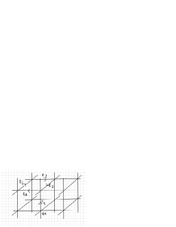
Figure 2: Electric Field Link Variables

A simulation algorithm for this system is easily devised:

1. Pick starting lattice locations (randomly) for the $N$ particles of charge $q_{i},i=1,..N$. Then solve Gauss’ Law for these fixed charge locations to obtain a starting configuration of electric link field variables satisfying the Gauss constraint.

2. Update the electric fields by shifting all link variables along a complete set of independent closed paths by constant shifts. In the simplest version of this, one simply considers all plaquettes (unit squares) on the lattice, shifting the 4 link fields ordered around the plaquette by a random $\alpha,-\alpha_{\rm max}<\alpha<\alpha_{\rm max}$. This preserves Gauss’ law. In fact, for systems with constant dielectric, one may use [11] fast Fourier transform methods to effect a global update of the electric fields, completely eliminating autocorrelations.

3. Update particle locations by visiting in turn every site $\vec{n}$ containing a charged particle of charge $q_{i}$. A particle move to the neighboring site $\vec{n}+\hat{\mu}$ in a random direction $\mu$ is then considered, where the particle move is accompanied with a shift of the electric field $E_{l}$ on the link $l=(\vec{n}\rightarrow\vec{n}+\hat{\mu})$

   $$E_{l}\rightarrow E_{l}-q_{i}$$

   to maintain Gauss’ law. In practice [10], we need to couple particle moves to field changes on several neighboring links to get reasonable acceptance rates.

A classic example of a strongly coupled Coulomb gas is the case of two like charged plates (see Figure 3), with mobile counterions (rendering the system overall neutral) between the plates. For appropriate choice of the charge density $\sigma$ on the plates, the system can be switched from weakly to strongly coupled simply by doubling the valence of the counterions (i.e. half as many doubly charged ions). For singly charged ions one finds, using the local gauge simulation techniques described above, a positive pressure, as shown in Figure 4 (also shown is the dependence on lattice discretization for the same physical size system). Mean field theory, along the lines discussed previously in Section 2, always gives a repulsive plate interaction of this form. On the other hand, if we double the charge on each ion, leaving the plate charge density fixed (and halving the number of counterions), one then finds an attractive force between the like charged plates (negative pressure), implying a complete breakdown of the saddle-point expansion of Section 2. The result of a numerical simulation of this system using the local gauge method is shown in Fig. 5 (for details, see [10]), where the total pressure (solid line) is seen to be negative. These results agree with explicit (and painful) molecular dynamics simulations [15] of the like-charged-plate problem.

Figure 3: Coulomb gas between like charged plates

Figure 4: Plate pressure for univalent ions

Figure 5: Plate pressure for divalent ions

5 Inhomogeneous Dielectric Effects in Coulomb Gas Problems

In realistic situations, the dielectric field $\epsilon$ is NOT constant, but varies from 2-6 in the interior of macromolecules to 80 in the surrounding medium (water)

$$\vec{D}(\vec{r})=-\epsilon(\vec{r})\vec{\nabla}\phi(\vec{r})+\vec{\nabla}\times\vec{A}(\vec{r})\equiv\vec{D}^{||}(\vec{r})+\vec{D}^{\rm tr}(\vec{r})$$

Maxwell’s equations imply $\vec{D}^{\rm tr}=0$ but if this constraint is not explicitly imposed:

$$\int d\vec{r}\frac{\vec{D}^{2}}{\epsilon(\vec{r})}=\int d\vec{r}\frac{\vec{D}^{||}(\vec{r})^{2}}{\epsilon(\vec{r})}+\int d\vec{r}\frac{\vec{D}^{\rm tr}(\vec{r})^{2}}{\epsilon(\vec{r})}$$

Ignoring the irrotational constraint, if we procede as previously:

$$Z^{\prime} = \int\prod_{i=1}^{N}d\vec{r}_{i}\prod_{\vec{r}}{\cal D}\vec{D}(\vec{r})\delta(\vec{\nabla}\cdot\vec{D}-\rho(\vec{r}))$$

$$\cdot e^{-\frac{\beta}{2}\int d\vec{r}\vec{D}^{2}/\epsilon(\vec{r})}$$

$$=\int\prod_{i=1}^{N}d\vec{r}_{i}\prod_{\vec{r}}{\cal D}\vec{D}^{||}(\vec{r}){\cal D}\vec{D}^{\rm tr}(\vec{r})\delta(\vec{\nabla}\cdot\vec{D^{||}}-\rho(\vec{r}))$$

$$\cdot e^{-\frac{\beta}{2}\int d\vec{r}\vec{D}^{||}(\vec{r})^{2}/\epsilon(\vec{r})}e^{-\frac{\beta}{2}\int d\vec{r}\vec{D}^{\rm tr}(\vec{r})^{2}/\epsilon(\vec{r})}$$

The integral over $\vec{D}^{\rm tr}$ gives a spurious unphysical dependence on $\epsilon(\vec{r})$- which can change dynamically in the course of the simulation ($\epsilon(\vec{r})$ depends implicitly on $\vec{r}_{i}$). Regularizing the path integral with a spatial lattice, the exact form of the spurious $\epsilon$-dependence can be revealed simply by turning off all free charges so the contribution from the longitudinal part vanishes:

$${\cal F}(\epsilon) = \int\prod_{n\mu}dD_{n\mu}\delta(\bar{\Delta}_{\mu}D_{n\mu})e^{-\frac{\beta}{2}\sum_{n\mu}D_{n\mu}^{2}/\epsilon_{n\mu}}$$

$$=\int\prod_{n}d\lambda_{n}\prod_{n\mu}dD_{n\mu}e^{i\sum_{n}\lambda_{n}\bar{\Delta}_{\mu}D_{n\mu}-\frac{\beta}{2}\sum_{n}D_{n\mu}^{2}/\epsilon_{n\mu}}$$

$$=\int\prod_{n}d\lambda_{n}\prod_{n\mu}dD_{n\mu}e^{-i\sum_{n}D_{n\mu}\Delta_{\mu}\lambda_{n}-\frac{\beta}{2}\sum_{n}D_{n\mu}^{2}/\epsilon_{n\mu}}$$

$$=C\prod_{n\mu}\sqrt{\epsilon_{n\mu}}\int\prod_{n}d\lambda_{n}e^{-\frac{1}{2\beta}\sum_{n\mu}\epsilon_{n\mu}(\Delta_{\mu}\lambda_{n})^{2}}$$

$$=C^{\prime}\prod_{n\mu}\sqrt{\epsilon_{n\mu}}{\rm det}^{-\frac{1}{2}}(-\bar{\Delta}_{\mu}\epsilon_{\mu}\Delta_{\mu})$$

Evidently, in order to eliminate the spurious term, we need to include ${\cal F}^{-1}$ in the path integral:

$${\cal F}^{-1}(\epsilon)=\prod_{n\mu}e^{-\frac{1}{2}\sum_{n\mu}\log{(\epsilon_{n\mu}})}{\rm det}^{+\frac{1}{2}}(-\bar{\Delta}_{\mu}\epsilon_{\mu}\Delta_{\mu})$$

Including a positive power of the determinant of a local operator in a path integral is precisely the problem we face in unquenched QCD!

5.1 Eliminating transverse contributions with Lüscher multiboson fields

In the Lüscher approach to unquenched QCD, one begins with a polynomial approximation to $1/s$ in the interval $[0,1]$; a convenient choice is:

$$\frac{1}{s} \simeq C\prod_{k=1}^{N}((s-\mu_{k})^{2}+\nu_{k}^{2})$$

$$\mu_{k} = \frac{1}{2}(1+\delta)(1-\cos{\frac{2\pi k}{2N+1}})$$

$$\nu_{k} = \sqrt{\delta}\sin{\frac{2\pi k}{2N+1}}$$

implying for the determinant (scaling the spectrum to $[0,1]$) a corresponding approximation:

$${\rm det}^{+\frac{1}{2}}({\cal M})\simeq\prod_{k=1}^{N}{\rm det}^{-\frac{1}{2}}(({\cal M}-\mu_{k})^{2}+\nu_{k}^{2})$$

This leads to the corrected form for the path-integral:

$$Z = \int d\vec{r}_{i}dD_{n\mu}d\phi^{(k)}_{n}\delta(\bar{\Delta}_{\mu}D_{n\mu}-\rho_{n})$$

$$\cdot e^{-\frac{1}{2}\sum_{n\mu}\log{(\epsilon_{n\mu}})-\frac{\beta}{2}\sum_{n\mu}D_{n\mu}^{2}/\epsilon_{n\mu}}$$

$$\cdot e^{-\sum_{k=1}^{N}\phi^{(k)}(({\cal M}-\mu_{k})^{2}+\nu_{k}^{2})\phi^{(k)}}$$

The approximation only adequately describes the low eigenstates if one uses a sufficiently large number $N$ of auxiliary fields, which limits its usefulness in QCD, where the density of low eigenmodes of the Dirac operator is large, due to spontaneous symmetry breaking. Fortunately, in biophysical applications, the IR spectrum of the Poisson operator is sparse (unlike QCD) and we can get away with a small number of boson fields (as we shall se shortly, often $N$=4 is adequate).

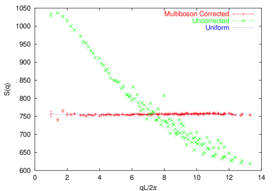
Figure 6: Structure Function for Neutral Dielectric Plasma

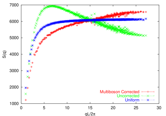
Figure 7: Structure Function for Charged Dielectric Plasma

A useful testbed for the multiboson implementation of a Coulomb gas with dynamical dielectric effects is the dielectric plasma, in which mobile particles (either neutral or charged) are assigned a dielectric constant different from that of the ambient medium. It is convenient to associate the dielectric field with links, each link being given a value depending on whether a particle is present at either, neither or both of the end sites of the link (for further details, see [12, 13]). An appropriate observable is the structure factor $S(q)\equiv\int d\vec{r}e^{i\vec{q}\cdot\vec{r}}<\rho(\vec{r})\rho(0)>$: for neutral particles, this must be $q$-independent. As a first test, consider a model with 1000 neutral dielectric particles, on a 16³ lattice, with a ratio of particle to background dielectric given by $\epsilon_{\rm part}/\epsilon_{\rm bg}$=0.2.

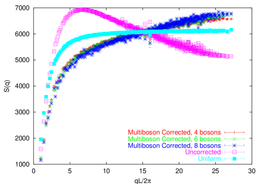
Figure 8: Dependence on number of multiboson fields

As we see in Figure 6, once the multiboson fields are included, the measured structure factor is indeed flat, to a very good approximation. A somewhat more realistic model is the 1 component charged dielectric plasma, on a 32³ lattice, with 8000 particles, and $\epsilon_{\rm part}/\epsilon_{\rm bg}$=0.05. In Figure 7 we show the results for such a plasma, with and without the contribution from the multiboson fields. Evidently, the results are qualitatively incorrect without taking into account the induced effects in the transverse electric field. In Figure 8, we show the dependence on the number of multiboson fields used. As remarked previously, it is remarkable how few fields are needed to achieve reasonable accuracy in this model.

6 Conclusions

The last 15 years has seen an extensive development in the theory of the thermodynamics of Coulomb gases, vastly extending the scope of treatable systems beyond the simplest cases to which elementary Debye-Hückel theory is applicable. The new methods treat a combined system of charged (and even multipolar) particles interacting with fields, and with both particles and fields realized on a discrete spatial lattice. Formally, the functional formalism for the grand-canonical partition function offers the greatest generality, but is restricted in usefulness to weakly coupled Coulomb gases. The local gauge formulation introduced by Maggs and Rossetto [9], and recently generalized to systems with dynamical dielectric by Coalson, Duncan and Sedgewick [12] allows the efficient simulation of strongly coupled Coulomb gases in a local formalism, circumventing the nonlocal Coulomb interaction which complicates, and frequently renders intractable, the molecular dynamics approach.

7 Acknowledgements

It is a pleasure to acknowledge the numerous colleagues from whom I have learned an enormous amount in the course of collaborations in the area of biophysics over the past 15 years: in particular, R. Coalson, R. Sedgewick, and S. Tsonchev, whose expertise and timely intervention have frequently averted scientific derailment. The research of A. Duncan is supported in part by NSF contract PHY-0554660.

References

[1] See, for example, D. A. McQuarrie, Statistical Mechanics
(Harper and Row, New York, 1976).
[2] E. J. W. Verwey and J. Th. G. Overbeek, Theory of the
Stability of Lyophobic Colloids (Elsevier, Amsterdam, 1948).
[3] R. D. Coalson and A. Duncan, J. Chem. Phys. 97, 5653(1992).
[4] N. Ben-Tal, R.D. Coalson, A. Duncan, and A. M. Walsh, J. Chem. Phys. 102, 4584(1995).
[5] R. D. Coalson and A. Duncan, J. Phys. Chem. 100, 2612(1996).
[6] R. D. Coalson, A. Duncan and S. Tsonchev, Phys. Rev. E60, 4257(1999).
[7] R. D. Coalson, A. Duncan and S. Tsonchev, Phys. Rev. E62, 799(2000).
[8] S-S Chern, R. D. Coalson, A. Duncan and S. Tsonchev, J. Chem. Phys. 113, 8381(2000).
[9] A. C. Maggs and V. Rossetto, Phys. Rev. Lett. 88, 196402(2002).
[10] R. D. Coalson, A. Duncan and R. D. Sedgewick, Phys. Rev. E71, 046702(2005).
[11] R. D. Coalson, A. Duncan and R. D. Sedgewick, Comput. Phys. Commun. 175, 73(2006).
[12] R. D. Coalson, A. Duncan and R. D. Sedgewick, Phys. Rev. E73, 016705(2006).
[13] A. Duncan and R. D. Sedgewick, Phys. Rev. E73, 066711(2006).
[14] A. G. Moreira and R. R. Netz, Eur. Phys. Jour. E8, 33(2002).
[15] L. Guldbrand, B. Jönsson, H. Wennerström and P. Linse,
J. Chem. Phys. 80, 2221(1984).