An analysis of the hadronic spectrum from lattice QCD.

W. Armour

2004

Department of Physics, University of Wales Swansea, Swansea SA2 8PP, Wales

Abstract

In chapter 1 I begin by discussing the basic ideas of quantum field theory (QFT). I provide a review of symmetries in physics and then move on to discuss the quark model. Chapter 2 is a review of lattice gauge theory with particular attention paid to lattice QCD. I begin by introducing lattice QCD, I then discuss some of the associated problems. I move on to discuss gauge fields on the lattice along with free lattice fermions. I then use this to define the lattice QCD action. I conclude this chapter by discussing how to reproduce the correct continuum physics. Chapter 3 discusses the basic numerical techniques employed in lattice simulations. I review methods for putting particles onto the lattice and conclude with a discussion of how to fit the resulting data. Chapter 4 reviews symmetries of the QCD Lagrangian, various forms of symmetry breaking in physics, the PCAC relation, the Goldberger-Treiman relation and the spontaneous breakdown of the axial symmetry. I move on to discuss sigma models and finally arrive at a basic chiral perturbation theory. I present research completed with my supervisor C. Allton and collaborators A.W. Thomas, D.B. Leinweber and R. Young in chapters 5 & 6. This work involves making lattice predictions for the hadronic mass spectrum using extrapolation techniques based on the predictions of chiral perturbation theory which have been developed by the Adelaide group.

Declaration

This thesis is a presentation of the research work I completed in collaboration with C. Allton, R. Young, D.B. Leinweber and A.W. Thomas. This document was written entirely by me and typeset using LaTeX. Preliminary results from these calculations were presented at lattice 2003 and in

An analysis of the vector meson spectrum from lattice QCD,
W. Armour.,
hep-lat/0309053.

Chiral and Continuum Extrapolation of Partially-Quenched Lattice Results
C. R. Allton, W. Armour, D. B. Leinweber, A. W. Thomas, R. D. Young.,
Phys.Lett. B628 (2005) 125-130
hep-lat/0504022.

Unified chiral analysis of the vector meson spectrum from lattice QCD
W. Armour, C. R. Allton, D. B. Leinweber, A. W. Thomas, R. D. Young.,
hep-lat/0510078.

Chiral and Continuum Extrapolation of Partially-Quenched Hadron Masses
C. R. Allton, W. Armour, D. B. Leinweber, A. W. Thomas, R. D. Young.,
PoS(LAT2005)049.
hep-lat/0511004.

An analysis of the nucleon mass from lattice QCD,
W. Armour, C.R. Allton, D.B. Leinweber, A.W. Thomas, R. Young.
(In preparation)

This work has not previously been accepted in substance for any degree and is not being concurrently submitted in candidature for any degree.

Signed ……………………………………      (candidate)
Date …………………………………….

This thesis is the result of my own investigations, except where otherwise stated.
Other sources are acknowledged by footnotes giving explicit references. A bibliography is appended.

Signed ……………………………………      (candidate)
Date …………………………………….

I hereby give consent for my thesis, if accepted to be available for photocopying and for inter-library loan, and for the title and summary to be made available to outside organisations.

Signed ……………………………………      (candidate)
Date …………………………………….

Chapter 1 Introduction

1.1 Why Quantum Field Theory?

Although quantum mechanics was a pioneering theory, it was apparent to all that it failed on many different levels. The most basic failure of quantum mechanics is its inability to account for a relativistic system of particles. In such a system the number of particles is not conserved. Dirac knew that this inconsistency had to be resolved in order to correctly account for a real particle process. In 1927 he published a paper The quantum theory of the emission and absorption of radiation which was a first attempt at unifying the theory of special relativity with quantum mechanics. It was this paper that laid the foundations for a quantum theory of fields, all modern theories have their roots based in this. Quantum field theory has proved to be an amazingly successful framework for building theories of the fundamental forces of nature. Its predictions for the interactions between electrons and photons have proved to be correct to one part in $10^{8}$. Moreover in the form of the standard model, it explains three of the four fundamental forces of nature, electromagnetism and the strong and weak nuclear forces. The standard model only fails to explain the fourth fundamental force, gravity.

1.2 The path integral

The path integral is a very powerful method of quantisation and is of great use in QFTs. Here we review a simple example by considering the Hamiltonian for a quantum mechanical particle in one space dimension

$$H=\frac{p^{2}}{2m}+V(x)=H_{0}+V$$ (1.1)

In the Heisenberg representation we may write the transition amplitude as

$$\langle x^{\prime},t^{\prime}|x,t\rangle=\langle x^{\prime}|e^{-h(t^{\prime}-t)}|x\rangle$$ (1.2)

If we use the fact that $e^{a+b}=e^{a}e^{b}$ and insert a complete set of co-ordinate eigenstates,

$$\int dx_{1}|x_{1}\rangle\langle x_{1}|=1$$ (1.3)

between the exponentials, let $T=(t^{\prime}-t)$ and $\Delta t=(t_{1}-t)$, we then have

$$\langle x^{\prime},t^{\prime}|x,t\rangle=\int dx_{1}\langle x^{\prime}|e^{-iH(T-\Delta t)}|x_{1}\rangle\langle x_{1}|e^{-iH\Delta t}|x\rangle$$ (1.4)

Dividing $T$ into $n$ equal parts $(T=n\Delta t)$ and inserting $(n-1)$ states in this way we have

$$\langle x^{\prime},t^{\prime}|x,t\rangle = \int dx_{1}\ldots dx_{n-1}\langle x^{\prime}|e^{-iH\Delta t}|x_{n-1}\rangle$$ (1.5)

$$\langle x_{n-1}|e^{-iH\Delta t}|x_{n-2}\rangle\ldots\langle x_{1}|e^{-iH\Delta t}|x\rangle$$

For small $\Delta t$ the exponentials can be well approximated using only the first term of the Baker-Campbell-Hausdorff formula (eq. 2.30) allowing us to rewrite the matrix elements as

$$\langle x_{k+1}|e^{-iH\Delta t}|x_{k}\rangle\approx\langle x_{k+1}|e^{-iH_{0}\Delta t}e^{-iV\Delta t}|x_{k}\rangle=\langle x_{k+1}|e^{-iH_{0}\Delta t}|x_{k}\rangle e^{-iV\Delta t}$$ (1.6)

where we have used the fact that $V$ only depends on space co-ordinates. We can calculate the remaining matrix element by introducing a complete set of momentum eigenstates,

$$\int dp|p\rangle\langle p|=1$$ (1.7)

and making use of the fact that

$$\langle x|p\rangle=\frac{1}{2\pi\hbar}e^{\frac{ipx}{\hbar}}$$ (1.8)

By combining the remaining exponentials and completing the square we are left with a simple Gaussian integral, performing this gives

$$\langle x_{k+1}|e^{-iH_{0}\Delta t}|x_{k}\rangle e^{-iV\Delta t}=\sqrt{\frac{m}{2\pi i\hbar^{2}\Delta t}}\exp i\Delta t\biggr{\{}\frac{m}{2\hbar}\biggr{(}\frac{x_{k+1}-x_{k}}{\Delta t}\biggl{)}^{2}-V(x)\biggl{\}}$$ (1.9)

Hence our amplitude takes the form

$$\langle x^{\prime}|e^{-iHT}|x\rangle=\int\frac{dx_{1}\ldots dx_{n-1}}{\bigr{(}\frac{2\pi i\hbar^{2}\Delta t}{m}\bigl{)}^{\frac{n}{2}}}\exp i\sum_{k=0}^{n-1}\Delta t\biggr{\{}\frac{m}{2\hbar}\biggr{(}\frac{x_{k+1}-x_{k}}{\Delta t}\biggl{)}^{2}-V(x)\biggl{\}}$$ (1.10)

If we now consider the limit of $n\rightarrow\infty$ we see that the exponent becomes the classical action for the path $x(t)$ from $x$ to $x^{\prime}$.

$$\sum_{k=0}^{n-1}\Delta t\biggr{\{}\frac{m}{2\hbar}\biggr{(}\frac{x_{k+1}-x_{k}}{\Delta t}\biggl{)}^{2}-V(x)\biggl{\}}$$

$$\textrm{as }n\rightarrow\infty \int_{0}^{T}dt\biggr{\{}\frac{m}{2}\biggr{(}\frac{dx}{dt}\biggl{)}^{2}-V(x)\biggl{\}}={\cal S}$$ (1.11)

Finally we note that the integrations over the $x_{k}$ can be interpreted as an integration over all possible paths $x(t)$. To describe this we introduce the notation

$$\biggr{(}\frac{m}{2\pi i\hbar^{2}\Delta t}\biggl{)}^{\frac{n}{2}}dx_{1}\ldots dx_{n-1}\rightarrow const.\prod_{t}dx(t)={\cal D}x$$ (1.12)

Hence we may now write our quantum mechanical amplitude in the path integral representation as

$$\langle x^{\prime}|e^{-iHT}|x\rangle=\int{\cal D}x~{}e^{\frac{i{\cal S}}{\hbar}}$$ (1.13)

To make the transition to classical mechanics we simply take the limit $\hbar\rightarrow 0$. To make the transition to a three dimensional theory we simply generalise to paths $x_{i}(t)$

$${\cal D}x\rightarrow\prod_{t}\prod_{i}dx_{i}(t)$$ (1.14)

1.3 Quantum Field Theory

As discussed at the beginning of this chapter quantum field theory is the most successful frame work for describing the sub-atomic world. In section 1.2 we derived the path integral for a simple one dimensional quantum mechanical system. To move to a quantum field theory we must introduce the functional integral representation of quantum field theory. Although this can be derived rigorously, here I will motivate it by analogy. The key concept is to promote the basic variables, $x_{i}(t)$, of our quantum mechanical example to fields, $\psi(\vec{x},t)$. Our rules for the transition are then:

$$x_{i} \rightarrow \psi(x,t)$$

$$i \rightarrow \vec{x}$$

$$\prod_{t,i}dx_{i}(t) \rightarrow \prod_{t,\vec{x}}d\psi(\vec{x},t)={\cal D}\psi$$

$${\cal S}=\int dtL \rightarrow {\cal S}=\int d^{4}x{\cal L}$$ (1.15)

Here $L$ is the Lagrange function and $\cal L$ is the Lagrangian density, which from here on will be referred to the Lagrangian. The objects of interest in quantum field theory are the vacuum expectation values of field operators, also known as correlation functions or Green’s functions. These Green’s functions contain all physical information about the system. In analogy with our quantum mechanical path integral we can write a representation of the Green’s functions in terms of functional integrals:

$$\langle 0|O|0\rangle = \frac{1}{{\cal Z}}\int{\cal D}\psi\,Oe^{\frac{iS}{\hbar}}$$

$$\textrm{with}\qquad{\cal Z} = \int{\cal D}\psi\,e^{\frac{iS}{\hbar}}$$ (1.16)

We interpret this as an integration over all classical field configurations.

1.4 Symmetries

One of the major advantages of the Lagrangian formalism of QFT is that symmetries of the Lagrangian lead to conserved currents, also known as Noether currents. To exemplify this we consider a Lagrangian that is symmetric under some given transformation of the fields:

$$\psi \rightarrow \psi+\delta\psi$$

$$\partial_{\mu}\psi \rightarrow \partial_{\mu}\psi+\delta(\partial_{\mu}\psi)$$ (1.17)

For a symmetric Lagrangian we have:

$${\cal L}(\psi,\partial_{\mu}\psi) = {\cal L}(\psi+\delta\psi,\partial_{\mu}\psi+\delta(\partial_{\mu}\psi))$$

$$\textrm{Hence}\qquad\delta{\cal L} = {\cal L}(\psi+\delta\psi,\partial_{\mu}\psi+\delta(\partial_{\mu}\psi))-{\cal L}(\psi,\partial_{\mu}\psi)=0$$ (1.18)

$$= \frac{\partial{\cal L}}{\partial\psi}\delta\psi+\frac{\partial\cal L}{\partial(\partial_{\mu}\psi)}\delta(\partial_{\mu}\psi)$$

where we have Taylor expanded the first term to leading order in $\delta\psi$. Using $\delta(\partial_{\mu}\psi)=\partial_{\mu}(\psi+\delta\psi)-\partial_{\mu}\psi=\partial_{\mu}(\delta\psi)$, the equations of motion for a field and the rule for differentiating a product we have:

$$0 = \partial_{\mu}\biggl{(}\frac{\partial{\cal L}}{\partial(\partial_{\mu}\psi)}\biggr{)}\delta\psi+\frac{\partial{\cal L}}{\partial(\partial_{\mu}\psi)}(\partial_{\mu}\delta\psi)$$ (1.19)

$$= \partial_{\mu}\biggl{(}\frac{\partial{\cal L}}{\partial(\partial_{\mu}\psi)}\delta\psi\biggr{)}$$

$$= \partial_{\mu}J^{\mu}$$

Here $J^{\mu}$ is the conserved current. With this their is an associated conserved charge. To calculate this we integrate the conservation equation over all space:

$$0 = \int d^{3}x\partial_{\mu}J^{\mu}$$ (1.20)

$$= \int d^{3}x\partial_{0}J^{0}+\int d^{3}x\partial_{i}J^{i}$$

$$= \frac{\partial}{\partial t}\int d^{3}xJ^{0}+\int dS_{i}J^{i}$$

$$= \frac{\partial}{\partial t}Q+\textrm{surface term}$$

Assuming that our field $(\psi)$ vanishes at infinity, the surface term can be neglected. Hence a conserved current leads to a conserved charge. We will see the importance of these ideas in chapter 4.

1.5 The Quark model

1.5.1 The Eightfold Way

Oppenheimer once quipped “The Nobel Prize should be given to the physicist who does not discover a new particle”. He was referring to the seemingly endless discovery of new particles that was taking place during the 1960’s. Theoretical understanding of elementary particles during this period was a mess. Although Yukawa proposed a theory describing the strong interaction, it had a coupling constant that was very large and hence perturbation theory was unreliable. One important observation was that the existence of resonances usually indicated the presence of bound states. This lead Sakata [1] to postulate that the hadrons were composed of states built out of proton $(p)$, neutron $(n)$ and lambda $(\Lambda)$ particles. Ikeda, Ogawa and Ohnuki took this idea further by proposing that these particles transformed in the fundamental representation $(\bf{3})$ of $SU(3)$. They also stated that mesons could be built out of bound states of $\bf{3}$ and $\bf{\bar{3}}$ [2]. Unfortunately some of their assignments were incorrect though. The correct $SU(3)$ assignments were discovered by Gell-Mann and Ne’eman. They postulated that baryons and mesons could be arranged in what they called the “Eightfold way” [3]. Gell-Mann went on to propose (with Zweig) that the $SU(3)$ assignments could be generated by introducing new constituent particles called “quarks” which transformed as a triplet $\bf{3}$.

1.5.2 Strangeness

It had been observed that a new quantum number, in addition to the isospin quantum number, was also conserved by strong interactions. This was called strangeness, and could be explained in terms of the $SU(3)$ flavour group. This group has representations labelled by two numbers, the third component of isospin $(I_{3})$ and a new quantum number called hypercharge $(Y)$. The strangeness quantum number and hypercharge can be related to each other via the Gell-Mann–Nishijima formula [4], [5]:

$$Q=I_{3}+\frac{Y}{2}=\left(\begin{array}[]{ccc}\frac{2}{3}&0&0\\ 0&-\frac{1}{3}&0\\ 0&0&-\frac{1}{3}\\ \end{array}\right)$$ (1.21)

with $Y=B+S$, where $B$ is the baryon number, $S$ is the strangeness, and $Q$ is the charge.

1.5.3 A global $SU(3)$ symmetry

To fit the known hadronic spectrum of particles, it was proposed that mesons were formed from a quark and anti-quark, while baryons were formed from three quarks. Hence it was expected that mesons and baryons would be arranged according to the following tensor decompositions:

$$\begin{array}[]{lrcl}\textrm{Meson}&\qquad\bf{3}\otimes\bf{\bar{3}}&=&\bf{8}\oplus\bf{1}\\ \textrm{Baryon}&\qquad\bf{3}\otimes\bf{3}\otimes\bf{3}&=&\bf{10}\oplus\bf{8}\oplus\bf{8}\oplus\bf{1}\end{array}$$ (1.22)

To see how the bound states are constructed for the mesons we arrange the meson matrix according to their quark wave functions:

$$M = \bf{3}\otimes\bf{\bar{3}}=\left(\begin{array}[]{ccc}u\bar{u}&u\bar{d}&u\bar{s}\\ d\bar{u}&d\bar{d}&d\bar{s}\\ s\bar{u}&s\bar{d}&s\bar{s}\end{array}\right)$$ (1.26)

$$= \left(\begin{array}[]{ccc}(2u\bar{u}-d\bar{d}-s\bar{s})/3&u\bar{d}&u\bar{s}\\ d\bar{u}&(2d\bar{d}-u\bar{u}-s\bar{s})/3&d\bar{s}\\ s\bar{u}&s\bar{d}&(2s\bar{s}-u\bar{u}-d\bar{d})/3\end{array}\right)$$ (1.30)

$$+ (1/3)\mathbf{1}(u\bar{u}+d\bar{d}+s\bar{s})$$ (1.31)

Using this we can write the meson matrix for the pseudoscalar mesons as:

$$M=\left(\begin{array}[]{ccc}\frac{1}{\sqrt{2}}\pi^{0}+\frac{1}{\sqrt{6}}\eta&\pi^{+}&K^{+}\\ \pi^{-}&-\frac{1}{\sqrt{2}}\pi^{0}+\frac{1}{\sqrt{6}}\eta&K^{0}\\ K^{-}&\bar{K^{0}}&-\frac{2}{\sqrt{6}}\eta\\ \end{array}\right)$$ (1.32)

This octet may be represented graphically by plotting isospin against hypercharge. Figure 1.1 depicts this.

Figure 1.1: A graphical representation of the pseudoscalar meson octet. $I_{3}$ represents the third component of isospin and $Y$ is the hypercharge.

1.5.4 QCD

After many decades of confusion QCD emerged as the best candidate to describe the strong interaction. It has six flavours of quark in the fundamental representation, these can be arranged into three families $(u,d),(c,s)$ and $(t,b)$. Leptons can similarly be grouped into three $SU(2)$ doublets in electro-weak theory. It is unclear why there should only by three families in the standard model. QCD is based on the $SU(3)$ colour symmetry group. The eight generators of the group are represented by the Gell-Mann matrices $\lambda_{a},(a=1,\ldots,8)$. The gauge fields (gluon fields) are denoted by $A^{a}_{\mu}$. We express the gluon field strength tensor as:

$$G^{a}_{\mu\nu}=\partial_{\mu}A_{\nu}^{a}-\partial_{\nu}A_{\mu}^{a}+gf_{abc}A_{\mu}^{b}A_{\nu}^{c}]$$ (1.33)

The quarks are coupled to the gluon fields via the covariant derivative:

$$D_{\mu}=\partial_{\mu}+ig\lambda_{a}A^{a}_{\mu}$$ (1.34)

Putting this together we have the QCD Lagrangian:

$${\cal L}_{QCD}=-\frac{1}{4}G^{a}_{\mu\nu}G^{a\mu\nu}+\sum^{6}_{f,h=1}\bar{\psi}_{f}(i\not{D}-m_{fh})\psi_{h}$$ (1.35)

where the Yang-Mills field carries the $SU(3)$ colour force. The gauge group is unbroken and hence the force mediators (gluons), are massless. The quarks $(\psi_{f,h})$ carry a flavour index $(f,h)$ along with a colour index and Dirac index which I have suppressed.

1.6 A note on units and notation

Throughout this document we choose the natural system of units in which $\hbar=c=1$. We do this to simplify formulae and calculations. We may move back to conventional units via the following:

$$\hbar = 6.58\times 10^{-22}\quad\textrm{[MeV~{}sec]}$$

$$\hbar c = 1.97\times 10^{-11}\quad\textrm{[MeV~{}cm]}$$ (1.36)

Another useful conversion factor is:

$$\hbar c=197\quad\textrm{[MeV~{}fm]}$$ (1.37)

Which we shall employ when setting the scale in our simulations. Throughout this document we will frequently employ “slash notation” this is used because the product of the Dirac matrices with a four vector occurs so frequently. In the Minkowski metric it is defined by:

$$\gamma^{\mu}a_{\mu}=\gamma^{0}a_{0}+\gamma^{i}a_{i}=\not{a}$$ (1.38)

Chapter 2 Lattice QCD

In this chapter I review some of the fundamentals of lattice QCD. Detailed accounts of this subject can be found in [6] & [7].

2.1 An introduction to lattice gauge theory

Quantum Chromodynamics (QCD) is the leading candidate for a theory of the strong interaction. Unfortunately perturbation theory fails to reproduce nearly all of the low energy features of the hadronic world, an example of this would be the spectrum of the low lying hadron states. Perturbation theory only seems to be effective in the asymptotic region where comparisons between theory and experiment can be made. Non perturbative methods have proved to be very difficult in Quantum Field Theories (QFTs). One of the most powerful and elegant non-perturbative methods is Wilson’s Lattice Gauge Theory. In principle lattice gauge theory allows us to put QCD on a computer and calculate the basic features of the low energy strong interaction spectrum. This approach is only limited by available computational power. Monte-Carlo methods have proved very effective in producing predictions that roughly match experiment, and with computational power on average doubling every eighteen months the discrepancy between theory and experiment is ever decreasing.

2.2 The price we must pay

Putting QCD on a lattice comes with a price,

1. The metric is Euclidean. This means that lattice gauge theory calculations are limited to the static properties of QCD.

2. Lattice gauge theory explicitly breaks continuous and rotational invariance because space-time is discretised.

3. Lattice gauge theory is limited by available computational power, so we must work with quark masses that are far greater than actual physical masses. This also puts constraints on the volume of space-time that we can work in.

Some of these problems can be overcome by taking the continuum limit, this is where we let the lattice spacing $(a)\rightarrow 0$. We must also take an infinite volume limit. However the limitation of computational power means that currently lattice sizes are modest.

2.3 The path integral on a lattice

We begin by making a Wick rotation. Put simply if $(x^{0},x^{1},x^{2},x^{3})$ are coordinates in Minkowski space-time (with $x^{0}$ being the time coordinate) then we set:

$$x^{4}=ix^{0}$$ (2.1)

This can be thought of as a rotation in the complex time plane and gives us a imaginary value for our time coordinate. The new set of coordinates $(x^{1},x^{2},x^{3},x^{4})$ now have a Euclidean metric. The main benefit of doing this is that the action $(S)$ is now a real positive quantity and our phase factor (see eq. 1.3 becomes a real weighting and so can be interpreted as a probability.

2.4 Space-time discretisation

Lattice QCD relies on a discrete space-time. Discretising space-time removes the infinite number of degrees of freedom available to the fields and replaces them with a finite number. This allows the path integral (sec. 1.2) to be given an exact definition. We formulate our theory on a hyper-cubic lattice using the Euclidean coordinates $(x^{1},x^{2},x^{3},x^{4})$. Our lattice is typically defined by all of the points that obey:

$$\begin{array}[]{clll}&x^{i}&=&a~{}n^{i}\\ \textrm{where}&n^{i}&\in&\mathbb{Z}\\ \textrm{with}&0~{}\leq&n^{i}<&L\qquad\textrm{for}\ i=1,2,3\\ \textrm{and}&0~{}\leq&n^{4}<&T\end{array}$$ (2.3)

The spacing between lattice sites is known as the lattice spacing, $(a)$, and has dimensions of length. L is defined to be the length of the lattice measured in lattice units and is a dimensionless number. We apply periodic boundary conditions to the spatial dimensions and anti-periodic boundary conditions to the time dimension. This ensures Fermi-Dirac statistics. In doing so the momentum space is discretised, we have:

$$\begin{array}[]{rcl}p^{i}&=&\frac{2\pi}{aL}n^{i}\\ p^{4}&=&\frac{2\pi}{aT}(n^{4}+\frac{1}{2})\end{array}$$ (2.5)

Here the $n^{\mu}$ have the same constraints as before. The beauty of discretising space-time is that there is now a maximum allowable momentum. This means that lattice gauge theory has an ultra-violet cutoff and hence gauge theories on the lattice are naturally regularised.

2.5 Gauge fields on the lattice

We begin by defining a link between two neighbouring sites on our hyper-cubic lattice. We allow each link to have a dynamical degree of freedom which we denote by $U(n,n+\hat{\mu})=U_{ij}$ where $\hat{\mu}$ is the unit vector in the $\mu$ direction. The dynamical degree of freedom $U_{ij}$ belongs to the compact group $\mathbb{G}$, for example:

$$\begin{array}[]{lccl}Z_{2}:&U_{ij}&=&\pm 1\\ U(1):&U_{ij}&=&e^{i\theta}\\ SU(N):&U_{ij}&=&N\times N\;\textrm{matrix with}\;\mathrm{det}~{}U=1\;\&\;U^{\dagger}=U^{-1}\end{array}$$

We note that the link has an orientation:

$$U_{ij}^{\dagger}=U_{ij}^{-1}=U_{ji}$$ (2.6)

Hence taking the inverse reverses its direction.

At lattice point n we define the simplest closed path on the lattice, this is the plaquette. It is illustrated in fig 2.1.

Figure 2.1: The plaquette is the simplest closed path on the lattice.

Mathematically we have

$$U_{P}=U(n,n+\hat{\mu})U(n+\hat{\mu},n+\hat{\mu}+\hat{\nu})U(n+\hat{\mu}+\hat{\nu},n+\hat{\nu})U(n+\hat{\nu},n)$$ (2.7)

Using this we may now define the Wilson action for the gauge fields. This is just the sum over all distinct plaquettes, $P$.

$$S_{g}=\beta\sum_{P}(1-\textrm{Re~{}Tr}~{}U_{P})$$ (2.8)

For lattice gauge theory to predict properties of QFTs we must perform functional integrals (eq. 1.3) for example;

$$\begin{array}[]{cccl}&\langle O\rangle&=&\frac{1}{Z}\int{\cal D}U~{}O~{}e^{-S_{g}}\\ \textrm{where}&Z&=&\int{\cal D}U~{}e^{-S_{g}}\end{array}$$ (2.10)

Here ${\cal D}U$ is analogous to ${\cal D}A$ in eq 1.3. ${\cal D}U$ is called the Haar measure, it is defined as the product over all links:

$${\cal D}U=\prod_{i,j}~{}dU_{ij}$$ (2.11)

The Haar measure is a way to assign an invariant volume to subsets of locally compact topological groups. It has the following properties

$$\begin{array}[]{rclccl}\int dUf(U)&=&\int dUf(\Omega U)&=&\int dUf(U\Omega)&\quad\ \textrm{with}~{}\Omega\in\mathbb{G}\\ &&&&&\Rightarrow\textrm{left-right invariant.}\\ &&&&\\ \int dU&=&1&&&\Rightarrow\textrm{Normalisable.}\\ &&&&&\\ \int dU~{}U&=&0&&&\Rightarrow\textrm{Expectation value of}\\ &&&&&\quad\ \textrm{a gauge non-invariant}\\ &&&&&\quad\ \textrm{object is zero.}\end{array}$$ (2.13)

One important point to note is that on the lattice the volume of the gauge group is unity hence no gauge fixing is needed.

2.6 Free lattice fermions

I will now discuss the discretisation of the fermion fields. As we shall see this must be performed carefully to avoid the dreaded “fermion doubling problem”. We begin by considering a naive discretisation of the free fermion action:

$$S_{f}=\int\mathrm{d}^{4}x~{}\bar{\psi}(x)(\gamma^{\mu}\partial_{\mu}+m)\psi(x)$$ (2.14)

We note that the four dimensional integral may be represented as a sum as follows,

$$\int\mathrm{d}^{4}x\rightarrow a^{4}\sum_{n}$$ (2.15)

A symmetric difference approximation for $\partial_{\mu}\psi(x)$ is:

$$\partial_{\mu}\psi(x)=\frac{\psi_{n+\hat{\mu}}-\psi_{n-\hat{\mu}}}{2a}$$ (2.16)

Using eq 2.15 and substituting eq 2.16 into the free fermion action (eq 2.14) leads us to the lattice action for free fermions.

$$S_{f}^{\#}=\sum_{n}\biggl{[}~{}\frac{a^{3}}{2}\sum_{\mu=1}^{4}\bar{\psi}_{n}\gamma^{\mu}(\psi_{n+\hat{\mu}}-\psi_{n-\hat{\mu}})+ma^{4}\bar{\psi}_{n}\psi_{n}\biggr{]}$$ (2.17)

To calculate the lattice propagator we use a Fourier transform to move to momentum space. We find the lattice propagator in momentum space is given by:

$$\textrm{Propagator}^{-1}\sim\frac{1}{a}\sin(ak_{\mu})+m$$ (2.18)

This propagator has bad behaviour as we take the continuum limit ($a\rightarrow 0$). As we expect, the lattice propagator has a node at $k=0$, but it also has a node at the edge of the Brillouin zone $(k_{\mu}=\frac{\pi}{a})$ for each $\mu$. Hence the naive discretisation prescription has an unphysical doubling problem for each space-time dimension. Wilson proposed a convenient solution to this problem. He suggested that the lattice fermion action should be modified by hand. We may do this as long as the correct continuum limit is obtained. We add the following Wilson term to our previous naive action:

$$\frac{1}{2a}\bar{\psi}_{n}(\psi_{n+\hat{\mu}}+\psi_{n-\hat{\mu}}-2\psi_{n})$$ (2.19)

Calculating the momentum space contribution by Fourier transforming the fermion fields $(\psi)$ for this term and adding it to our previous naive action gives:

$$S_{Wf}^{\#}=\int\frac{\mathrm{d}^{4}k}{(2\pi)^{4}}\bar{\psi}(k)\Biggl{[}i\sum_{\mu}\gamma^{\mu}\frac{\sin(ak_{\mu})}{a}+m-\sum_{\mu}\frac{\cos(ak_{\mu})-1}{a}\Biggr{]}\psi(k)$$ (2.20)

The new cosine term preserves the minimum at $k=0$ but eliminates the unwanted minimum at the edge of the Brillouin zone. This solution to the doubling problem does come with a price, and that is the Wilson term breaks chiral symmetry at finite lattice spacing.

2.7 The lattice QCD action

The lattice QCD Lagrangian contains the following fields:

$$\begin{array}[]{rcll}\psi(n)&=&[\psi_{c,\alpha}^{f}](n)&\textrm{Quark fields having flavor:}~{}f=1,\ldots,N_{f}\\ &&&\textrm{Colour:}~{}c=1,2,3\quad\textrm{\&}\quad\textrm{Dirac index:}~{}\alpha=1,\ldots,4\\ U(n,n+\hat{\mu})&\in&SU(3)&\textrm{link variables:}~{}\mu=1,\ldots,4\end{array}$$ (2.22)

It is constructed to be invariant under an $SU(3)$ gauge transformation. The gauge transformations for the fields are as follows

$$U^{\prime}(n,n+\hat{\mu}) = \Omega(n)~{}U(n,n+\hat{\mu})~{}\Omega^{\dagger}(n+\hat{\mu})$$

$$\psi^{\prime}(n) = \Omega(n)~{}\psi(n)$$

$$\bar{\psi}^{\prime}(n) = \bar{\psi}(n)~{}\Omega^{\dagger}(n)$$ (2.23)

where the $\Omega(n)$ are $SU(3)$ matrices. The Wilson action for QCD is

$$S_{QCD}=S_{g}[U]+S_{q}[U,\psi,\bar{\psi}]\hskip 14.22636pt$$ (2.24)

The gauge action ($S_{g}[U]$) is given by equation 2.8 and the quark action ($S_{q}[U,\psi,\bar{\psi}]$) is given by

$$S_{q}[U,\psi,\bar{\psi}]=\bar{\psi}_{x}\mathrm{K}_{xy}\psi_{y}$$ (2.25)

where $\mathrm{K}_{xy}[U]$ is the quark matrix. The $x,y$ indices represent space-time, colour, spin and flavour. The quark matrix is given by equations 2.17 & 2.19, and introducing a gauge interaction.

$$\mathrm{K}_{xy}[U]=\delta_{xy}-\kappa\sum_{\mu}\biggl{[}\delta_{x,y-\hat{\mu}}(r-\gamma_{\mu})U_{x,\mu}+\delta_{x-\hat{\mu},y}(r+\gamma_{\mu})U^{\dagger}_{y,\mu}\biggr{]}$$ (2.26)

Wilson’s choice for $r$ is one. and in this case there is no species doubling. The spinor indicies are carried by the gamma matrices, the colour indices by the link variables and there is a Kronecker delta in flavour space, all of which are suppressed. The hopping parameter ($\kappa$) is related to the free quark mass by

$$\kappa=\frac{1}{2m+8}$$ (2.27)

2.8 The continuum limit

For our formalism of lattice gauge theory to be correct it must reproduce the correct continuum physics when we take the continuum limit. Here we briefly outline this for the gauge part of the action $(S_{g}[U])$. The first step in doing this for $\mathbb{G}=SU(N)$ is to use the fact that a unitary matrix may be written as the exponential of an imaginary matrix:

$$\begin{array}[]{lrcll}&U_{\mu}(n)&=&\exp\left(iag\frac{\lambda^{\alpha}}{2}A_{\mu}^{\alpha}(n)\right)&\\ &&&&\\ Where&g&=&\textrm{Coupling constant}&\\ &\lambda^{\alpha}&=&\textrm{generators of the gauge group }&\\ &A_{\mu}^{\alpha}(n)&=&\textrm{The gauge fields}&\end{array}$$ (2.29)

We then use the Baker-Campbell-Hausdoff formula to rewrite our plaquatte, $U_{P}$ (eq 2.7), as a single exponential.

$$e^{A}e^{B}=e^{A+B+\frac{1}{2}[A,B]+...}$$ (2.30)

We then use the fact that in continuum

$$[A_{\nu}(x),A_{\mu}(x+\hat{\nu})] = [A_{\nu}(x),A_{\mu}(x)]\hskip 125.19212pt$$

$$[A_{\nu}(x),A_{\nu}(x+\hat{\mu})] = [A_{\nu}(x),A_{\nu}(x)]=0$$ (2.31)

to identify the combined exponent with the Yang-Mills field strength tensor:

$$F_{\mu\nu}(x)=\partial_{\mu}A_{\nu}(x)-\partial_{\nu}A_{\mu}(x)+ig[A_{\mu}(x),A_{\nu}(x)]$$ (2.32)

We then take the trace of the plaquette by expanding the exponential. Next we define the Lie algebra for $\mathbb{G}$

$$\hskip 108.12047pt\begin{array}[]{rcl}[\lambda^{\alpha},\lambda^{\beta}]&=&2if^{\alpha\beta\gamma}\lambda^{\gamma}\\ \hskip 2.84526pt\mathrm{tr}(\lambda^{\alpha}~{}\lambda^{\beta})&=&2\delta^{\alpha\beta}\end{array}$$

and use it to show

$$tr[F_{\mu\nu}(x)^{2}]=\frac{1}{2}F_{\mu\nu}^{\alpha}F^{\mu\nu\alpha}$$ (2.33)

We then use $tr(U_{P})$ and equation 2.15 to rewrite the lattice action. Finally, it can be shown that the correct continuum physics expression is reproduced as we let $a\rightarrow 0$.

2.9 Setting the scale

Throughout this chapter our discussion of lattice QCD has been in lattice units, i.e. we rescale the fields and masses by appropriate powers of the lattice spacing to render them dimensionless. This is of no real use if we wish to make physical predictions that we may compare with experimental values. To be able to do this we must give our lattice predictions their correct dimensions. This is called setting the scale. The continuum value of an observable ($O_{cont}$), is given by

$$O_{cont}=\lim_{a\rightarrow 0}\frac{O_{\#}(a)}{a^{N}}$$ (2.34)

where $O_{\#}$ is our lattice observable and $N$ is the energy dimension of $O_{cont}$.

Massless lattice QCD contains one free parameter ($\beta$), so we use one observable to determine the lattice spacing ($a$). We may then make physical predictions based on our lattice simulations. In massive lattice QCD additional observables are needed to set the quark mass. More generally additional parameters are needed as more parameters are introduced.

Chapter 3 Numerical Methods

3.1 The effective gauge action

To compute observables in QCD we define the expectation value of an arbitrary operator $O$ as:

$$\langle O\rangle = \frac{1}{\cal Z}\int{\cal D}U{\cal D}\psi{\cal D}\bar{\psi}~{}O~{}e^{-S_{g}-S_{q}}$$

$$\cal Z = \int{\cal D}U{\cal D}\psi{\cal D}\bar{\psi}~{}e^{-S_{g}-S_{q}}$$ (3.1)

Grassmann variables cannot be modelled on a computer. Hence we cannot use any computational method which involves an action that contains Grassmann variables. We can however analytically integrate out the fermion fields from the functional integral ($\cal Z$).

$$\langle O\rangle = \frac{1}{\cal Z}\int{\cal D}U~{}O~{}e^{-S_{g}}\det K$$

$$\cal Z = \int{\cal D}Ue^{-S_{g}}\det K$$ (3.2)

Doing this leaves us with a functional integral over the gauge fields which may be expressed as integrals over real numbers. These can be handled on a computer with relative ease.

We are now ready to introduce an effective action, $S_{eff}$, by making use of the following identity:

$$\det X=e^{\ln\det X}=e^{\mathrm{Tr}\ln X}$$ (3.3)

So that we now write the integrand of equations 3.1 as:

$$S_{eff}=S_{g}-\ln(\det~{}K)=S_{g}-\mathrm{Tr}\ln K$$ (3.4)

3.2 The quark propagator

The quark propagator is a simple example of integrating out the fermion fields leaving us with an object that can be calculated on the lattice. The quark propagator is defined as the expectation value of the product of a $\psi$ and a $\bar{\psi}$ field.

$$\langle\psi_{x}\bar{\psi}_{y}\rangle=\frac{1}{\cal Z}\int{\cal D}\psi_{x}{\cal D}\bar{\psi}_{y}{\cal D}Ue^{-S_{g}-S_{q}}\psi_{x}\bar{\psi}_{y}$$ (3.5)

As before (sec 2.7) the $x,y$ indices represent space-time, colour, spin and flavour. The $S_{g}~{}\&~{}S_{q}$ represent the gluonic and quark parts of the lattice QCD action respectively. We note that the propagator is not gauge invariant because we may apply independent gauge transformations at each $x,y$ point. Performing the fermion integration yields:

$$\langle\psi_{x}\bar{\psi}_{y}\rangle=\frac{1}{\cal Z}\int{\cal D}Ue^{-S_{eff}}K^{-1}_{xy}$$ (3.6)

We may now define the quark propagator, $G=K^{-1}$, for a given gauge configuration U.

$$G^{\alpha\beta}_{12}(x,y;U)K_{(\beta,2,y),(\gamma,3,z)}[U]=\delta_{\alpha\gamma}\delta_{13}\delta_{xz}$$ (3.7)

The Greek indices represent spin, the numbers represent colour and the roman indices represent space-time co-ordinates. The flavour dependence of $G$ is a Kronecker delta and so is suppressed. Repeated indices should be summed over. This equation (eq. 3.7) can be solved using a matrix inversion algorithm such as the conjugate gradient method.

3.3 Monte Carlo simulations

Lattice gauge theory made a great leap forward when the Monte Carlo method was introduced. This is because a naive calculation of the path integral is prohibitive, since the sum contains a massive number of terms. To exemplify this consider the simplest group that we can define on the lattice, $\mathbb{Z}_{2}$ with elements $\pm 1$. If our lattice had $8^{4}$ sites then the path integral sum would contain the following number of terms:

$$2^{2^{14}}=2^{16384}\approx 10^{5460}$$ (3.8)

Since the number of links is $4\times 8^{4}=2^{14}$.

The Monte Carlo method is an example of importance sampling. It applies certain approximations to the path integral which alleviates this problem. Normally the path integral sums over an enormous amount of configurations that make an insignificant contribution to the integral. If we could ignore those configurations and only sum over the ones where the action is near its minimum, then our calculation would be much quicker. The Monte Carlo method does exactly this. We define a set of initial values for each link on the lattice ($\Sigma_{1}$). Then the Monte Carlo method tells us to generate a sequence of configurations $\Sigma_{2},\Sigma_{3}\ldots$ such that when statistical equilibrium is reached the probability of encountering a particular configuration $\Sigma_{i}$ in the sequence is proportional to the corresponding Boltzmann weight, $W_{i}=e^{-S[\Sigma_{i}]}$. The smaller set of configurations that we now use $\{\Sigma_{i}\}$ are those that are near minimum action and hence contribute most to the path integral.

3.4 The Metropolis algorithm

A common method for generating the sequence of configurations $\{\Sigma_{i}\}$ is the Metropolis algorithm [6]. Consider generating a new configuration $\sigma_{1}^{{}^{\prime}}$ from the configuration $\sigma_{1}$ by updating a single link using some random process. It is possible to calculate the change in the action via equation 3.9.

$$\Delta S=S(\sigma_{1}^{{}^{\prime}})-S(\sigma_{1})$$ (3.9)

A random number $r$ is now chosen between 0 and 1. If $e^{-\Delta S}>r$ then the configuration is accepted, if not it is rejected. If $\Delta S$ is negative then the change is always accepted because $e^{-\Delta S}>1$. If however we only accepted negative values of $\Delta S$ then the action would be constantly decreasing and hence would tend towards the classical equations of motion. Of course this is to be avoided because it neglects all quantum corrections.

By choosing a random number ($r$), we are actually allowing for positive $\Delta S$, hence the action may increase as we change from $\sigma_{1}$ to $\sigma_{1}^{{}^{\prime}}$. This allows for quantum fluctuations around the classical equations of motion. The algorithm progresses by moving to the next lattice site and changing it in some random way. Hence another configuration is generated, we test this to see if it meets the proper criteria and move on. In this way we sweep through the entire lattice successively making small changes. After many sweeps through the lattice we begin to reach thermal equilibrium, this yields the set of link variables $\Sigma_{1}$. The process is then repeated and the second set of link variables $\Sigma_{2}$ is obtained, and so on. Slowly a set of configurations is built up $\{\Sigma_{i}\}$. The effect of the algorithm is that the new configuration $\sigma_{1}^{{}^{\prime}}$ is accepted with the conditional probability of $e^{-\Delta S}$.

3.5 The quenched approximation

As seen in section 3.2, $S_{eff}$ is the correct action for lattice QCD. Unfortunately the second term in equation 3.4 makes the action non-local. This means that generating a sequence of configurations (sec. 3.3 & 3.4) is far more computationally demanding than generating a sequence of configurations for an action that is local. This is because we have to calculate the determinant of the quark matrix in the non-local case. By replacing the determinant in equation 3.4 with a constant that is independent of the gauge fields we have a modified the action which is now local. This is called the quenched approximation. In practice we set $\det K=1$ in equation 3.4 which modifies the effective action so that $S_{eff}=S_{g}$. This corresponds to setting the hopping parameter (sec. 2.7) to zero. This leaves us with infinitely heavy quarks which do not contribute to the effective action. This effect is countered by adjusting the remaining parameters of the theory. Although this seems like a very crude thing to do, it works surprisingly well with most of the essential features of QCD  remaining. Quenched results of calculations of the light hadron spectrum are within  10% of experimental results.

3.6 Hadron correlators

Correlation functions are used to measure many physical observables on the lattice.

$$C(x,y)=\langle O(x)O^{\dagger}(y)\rangle=\frac{1}{\cal Z}\int{\cal D}UO(x)O^{\dagger}(y)e^{-S_{eff}}$$ (3.10)

Here $O(x)$ is an interpolating operator. Any gauge invariant combination of fermion fields and gauge links can be used as a interpolating operator. As above this multi-dimensional integral is well approximated by the Monte-Carlo method (sec. 3.3) allowing us to represent the correlation function as the average of the operator $O(x)O^{\dagger}(y)$ evaluated on each of the independent configurations $\{\Sigma_{i}\}$:

$$\langle O(x)O^{\dagger}(y)\rangle\approx\frac{1}{N_{c}}\sum^{N_{c}}_{i=1}{\cal M}(\Sigma_{i})$$ (3.11)

Where ${\cal M}(\Sigma_{i})$ is the value of the operator $O(x)O^{\dagger}(y)$ calculated using the configuration $\Sigma_{i}$, $N_{c}$ is the number of configurations and $i$ represents the $i^{th}$ configuration in the sequence of configurations $\Sigma$.

3.6.1 Mesons

To place mesons on the lattice we use interpolation operators, $O(x)$, which are used to create and annihilate mesons. An operator for the meson state $|\cal M\rangle$ must satisfy:

$$\langle 0|O(x)|\cal M\rangle \neq 0$$

$$\langle 0|O(x)|\cal M^{\prime}\rangle = 0$$ (3.12)

Where $|\cal M^{\prime}\rangle$ is any state that is lighter than state $|\cal M\rangle$. This ensures that the operator has a non-zero overlap with the state that it is intended to represent and has no overlap with any lighter states. For the operator to be gauge invariant we require:

$$O(x)_{\beta g}^{\alpha f}=\delta_{a}^{b}\psi_{x}^{a\alpha f}\bar{\psi}_{x}^{b\beta g}$$ (3.13)

With $\alpha$ & $\beta$ being the Dirac index, $a$ & $b$ the colour index, $f$ & $g$ the flavour index and $x$ is the space-time co-ordinates. Since $\int d\Omega_{x}\Omega_{x}=0$ it follows that the expectation value of a meson propagator is zero unless $x=y$. To define a particular type of meson (pseudoscalar or vector) we pick an interpolating operator with the same quantum numbers as that type of meson. It is convenient to represent mesons in written form using the following combination of quantum numbers, $J^{PC}$. Table 3.1 gives a description of these numbers and their corresponding formulae.

Quantum number	Description	Formula
$J$	Total angular momentum	$J=(l+s,l+s-1,\ldots,|l-s|)$
$P$	Parity number	$P=(-1)^{l+1}$
$C$	Charge conjugation	$C=(-1)^{l+s}$

Table 3.1: This table contains a description of the $J^{PC}$ quantum numbers. The orbital angular momentum eigenvalue is represented by $l$ and the spin eigenvalue is represented by $s$.

Table 3.2 gives examples of the $J^{PC}$ numbers for some well known pseudoscalar and vector mesons.

	Meson	$J^{PC}$
	$\pi$	$0^{-+}$
	$\rho$	$1^{--}$
	$\sigma$	$0^{++}$
	b1	$1^{+-}$
	a1	$1^{++}$
	a2	$2^{++}$

Table 3.2: Some of the well known mesons and their $J^{PC}$ quantum numbers.

As an example we consider the following interpolation operator:

$$O(x,t)=\bar{\psi}_{f}(x,t)\gamma_{5}\psi_{g}(x,t)$$ (3.14)

This operator (Eq. 3.14) has the same $J^{PC}$ quantum numbers as the $\pi$-meson (pion). It is a local operator because the quark and anti-quark fields are at the same site $(x,t)$. It has been shown that for some mesons such as the $\rho$-meson an interpolation operator that also includes some form of wave function between the quark and anti-quark fields gives a better signal or overlap. This technique is known as smearing. Another technique involves the addition of bent paths to the original paths between quark and anti-quark, this is known as fuzzing. We can combine these interpolation operators to form mesons on the lattice. Substituting these operators into equation 3.10 represents a physical process in which a pion is created at the space-time point $(0,0)$, from there it propagates in space-time to the point $(x,t)$ where it is destroyed. This is pictorially illustrated in figure 3.1.

Figure 3.1: A pictorial representation of a meson correlator on the lattice. The meson is created at position and time $(0,0)$ and is destroyed at $(x,t)$.

The correlator can give us lots of information about the particle that we wish to study. As an example we will consider the local pion correlator. We begin by inserting our interpolation operator (Eq. 3.14) into the correlation function (Eq. 3.10). We have:

$$C_{\pi}(x,t;0,0)=\langle 0|{\cal T}\bar{\psi}_{f}(x,t)\gamma_{5}\psi_{g}(x,t)\bar{\psi}_{f}(0,0)\gamma_{5}\psi_{g}(0,0)|0\rangle$$ (3.15)

Where we have set $(y,t)=(0,0)$ and $\cal T$ represents time ordering. Next we perform a Wick contraction,

$$C_{\pi}(x,0;0,0) = \frac{1}{\cal Z}\int{\cal D}Ue^{-S_{eff}}\textrm{Tr}(G_{f}(0,x)\gamma_{5}G_{g}(x,0)\gamma_{5})$$ (3.16)

Here the sea quarks are contained in $S_{eff}$ and the valence quarks are contained in the quark propagators $G_{f}(0,x)~{}\&~{}G_{g}(x,0)$ (sec. 3.2). This is an example of a point to point correlator. As such its momentum is undefined. We may represent this integral using the Monte-Carlo approximation. If we treat quark flavors $g$ and $f$ as degenerate we have:

$$C_{\pi}(x,0)=\frac{1}{N_{c}}\sum_{i}^{N_{c}}\textrm{Tr}(G(0,x)\gamma_{5}G(x,0)\gamma_{5})$$ (3.17)

We will now use this to study the time slice correlator and show how to extract an estimate for the effective mass of the pion. We begin by performing a Fourier transform over the three spatial dimensions, $x$, (i.e. over a time slice). This fixes the momentum.

$$C_{\pi}(t,p)=\sum_{x}C_{\pi}(x,t;0,0)e^{ip.x}$$ (3.18)

Inserting a complete set of energy eigenstates that have the norm:

$$\sum_{n}\int\frac{d^{3}q_{n}}{2E_{n}}|n,q_{n}\rangle\langle n,q_{n}|=1$$ (3.19)

gives:

$$C_{\pi}(t,p)=\int\frac{d^{3}q_{n}}{2E_{n}}\sum_{x,n}\langle 0|O(x,t)|n,q_{n}\rangle\langle n,q_{n}|O^{\dagger}(0,0)|0\rangle e^{ip.x}$$ (3.20)

We now make use of the fact that a quantum operator $\cal O$ in the Heisenberg picture is time dependent ${\cal O}(x)={\cal O}(0)e^{-iE_{n}t-iq_{n}.x}$ and the fact that $\langle A|O|B\rangle=(\langle B|O^{\dagger}|A\rangle)^{*}$ inserting this in Eq. 3.20 gives:

$$C_{\pi}(p,t)=\int\frac{d^{3}q_{n}}{2E_{n}}\sum_{x,n}|\langle 0|O(0,0)|n,q_{n}\rangle|^{2}e^{-iE_{n}.t}e^{-i(q_{n}-p).x}$$ (3.21)

We may now simplify this by noting $\sum_{x}e^{-i(q_{n}-p).x}=\delta(q_{n}-p)$ and $\int d^{3}q_{n}\delta(q_{n}-p)$ implies $p=q_{n}$. We also rotate to Euclidean space $it\rightarrow t$. This leads to

$$C_{\pi}(p,t)=\sum_{n}\frac{|\langle 0|O(0)|n,p\rangle|^{2}}{2E_{n}}e^{-E_{n}.t}$$ (3.22)

Since we are in Euclidean space the correlator is exponentially damped in time so as $t\rightarrow\infty$ the lightest meson state dominates ($n=1$).

To extract a mass prediction we work in the rest frame (i.e. we set $p=0$). We define the effective mass as:

$$M^{eff}_{\pi}=\ln\biggl{(}\frac{C_{\pi}(t)}{C_{\pi}(t+1)}\biggr{)}$$ (3.23)

Plotting this against time allows us to gain a lattice estimate for the pion mass by looking for a plateau in the data. To convert this into a physical value we must set the scale (sec. 2.9). In practice the hadron mass is obtained by fitting $c(0,t)$ to an exponential over a time range where the ground state dominates.

3.6.2 Baryons

We place baryonic particles on to the lattice in much the same way as we did mesons. To define gauge invariant baryon fields we require:

$$O(x)^{\alpha f\beta g\gamma h}=\epsilon_{abc}\psi_{x}^{a\alpha f}\psi_{x}^{b\beta g}\psi_{x}^{c\gamma h}$$ (3.24)

We can prove that this is gauge invariant by suppressing all but the colour indices, and applying a gauge transformation:

$$\epsilon_{abc}\psi^{a}\psi^{b}\psi^{c}\rightarrow\epsilon_{abc}\Omega_{a^{\prime}}^{a}\Omega_{b^{\prime}}^{b}\Omega_{c^{\prime}}^{c}\psi^{a^{\prime}}\psi^{b^{\prime}}\psi^{c^{\prime}}$$ (3.25)

Gauge invariance follows from $\epsilon_{abc}\Omega_{a^{\prime}}^{a}\Omega_{b^{\prime}}^{b}\Omega_{c^{\prime}}^{c}=\det(\Omega)=1$.

As for the mesonic case, we construct interpolation operators with the quantum numbers of the particle that we wish to study. An example for the $\Delta^{++}$ would be:

$${\cal B}^{fgh}(x,t)=\epsilon_{abc}(C^{\dagger}\gamma_{\mu})_{\beta\gamma}\psi^{a\alpha f}_{x}\psi^{b\beta g}_{x}\psi^{c\gamma h}_{x}$$ (3.26)

With $C$ being the charge conjugation matrix $\bar{\psi}^{(c)}=-(C^{\dagger}\psi)^{T}$. This is an antisymmetric unitary $4\times 4$ matrix that relates $\gamma^{\mu}$ to its transpose. Explicitly we set $\psi^{f}=\psi^{g}=\psi^{h}=u$ with $u$ being an up quark. As before (sec. 3.6.1) we may use these interpolation functions to form baryon correlation functions and using similar techniques we can extract physical information about baryonic states.

3.7 Fitting the data

In any lattice calculation a set of observables $O_{i}$ are calculated on a number of configurations. To extract physical observables we fit the data to a particular function or model. This is done by the minimisation of the $\chi^{2}$ value. In our study we work with uncorrelated data. We define $\chi^{2}$ as:

$$\chi^{2} = \sum^{N}_{i=1}\biggl{[}\frac{y_{i}-f(x_{i},\{\alpha_{j}\})}{\sigma_{i}}\biggr{]}^{2}$$ (3.27)

$$\textrm{Where}\qquad x_{i} =$$ independent variable

$$y_{i} =$$ dependent variable

$$f(x_{i},\{\alpha_{j}\}) =$$ fitting function / model

$$N =$$ number of data points

$$\sigma_{i} = i^{th}$$ uncertainty of the data point

The $\chi^{2}$ is minimised by the set of independent variables that satisfy equation 3.28

$$\frac{\partial\chi^{2}}{\partial\alpha_{j}}=0$$ (3.28)

If the function $f(x_{i})$ is linear then equation 3.28 may be solved analytically, otherwise we must minimise $\chi^{2}$ numerically. In our study we quote values of reduced $\chi^{2}$ also known as $\chi^{2}$ per degree of freedom ($\chi^{2}/d.o.f$). This can be defined as:

$$\chi^{2}/d.o.f = \frac{1}{N-m}\sum^{N}_{i=1}\biggl{[}\frac{y_{i}-f(x_{i})}{\sigma_{i}}\biggr{]}^{2}$$ (3.29)

$$\textrm{Where}\qquad m =$$ number of fit parameters

An acceptable fit should have a $\chi^{2}/d.o.f$ of about one.

3.8 Statistical errors

We can associate an error with the fit parameters known as the statistical error. In the limit of an infinite number of gauge configurations we expect this to go to zero. Typically a lattice simulation has a small number of configurations $\cal O$(few hundred) this is because configurations are computationally expensive to generate, especially dynamical ones (sec. 3.5). Consequently it is important to quantify any error due to this. To do this we use bootstrap error analysis [8]. We begin by creating a bootstrap sub-ensemble by selecting $n$ configurations at random. Next the fitting procedure is applied to this sub-ensemble, in the same way it is for the true sample. This gives a new estimate for the fit parameters. We repeat this procedure $n_{boot}$ times. Doing this generates a bootstrap distribution for each of the fit parameters. Representing this as a histogram allows the central $67\%$ region to be defined and hence the upper and lower error bars.

Chapter 4 An introduction to Chiral Perturbation Theory

In this section we will review the symmetries of the QCD Lagrangian. We will then show how these symmetries can be exploited so that we can build an effective Lagrangian that can be used to describe the low energy dynamics of QCD.

4.1 Symmetries of the QCD Lagrangian

Along with the $U(1)$ symmetries that give rise to the conservation of baryon number, charge and strangeness (eq. 4.4), there exist two other interesting symmetries of the QCD Lagrangian, namely the Vector and Axial-Vector symmetries.

$$\begin{array}[]{rcll}\psi&\rightarrow&e^{-i\alpha B}\psi&\textrm{B is the baryon number of }\psi\\ \psi&\rightarrow&e^{-i\beta Q}\psi&\textrm{Q is the charge of }\psi\\ \psi&\rightarrow&e^{-i\epsilon S}\psi&\textrm{S is the strangeness of }\psi\\ \end{array}$$ (4.4)

$$\textrm{where}~{}\alpha,~{}\beta~{}\&~{}\epsilon~{}\textrm{are arbitrary real numbers}$$ (4.5)

4.1.1 The Vector symmetry

We will begin by considering the case of massless QCD. Here we need only consider a Lagrangian of the form:

$${\cal L}_{massless}=\bar{\psi}\not{D}\psi$$ (4.6)

I have suppressed all indices and ignored the gauge fields as they will not be influenced by the transformations that we will consider.

The vector transformation $(\Lambda_{V})$ which belongs to the group $SU(2)_{V}$ is defined by,

$$\psi \rightarrow \>\>\;\exp\Biggl{(}-i\frac{1}{2}\tau^{a}\theta^{a}\Biggr{)}\psi$$

$$\bar{\psi} \rightarrow \bar{\psi}\exp\Biggl{(}i\frac{1}{2}\tau^{a}\theta^{a}\Biggr{)}$$ (4.7)

Where $\tau^{a}$ are the Pauli iso-spin matrices. It is immediately obvious that our massless Lagrangian (eq. 4.6) will be invariant under this transformation since the transformation, $\Lambda_{V}$, has no space-time dependency. Hence our Lagrangian is $SU(2)$ flavour (iso-spin) invariant.

As was demonstrated in section 1.4, symmetries of the Lagrangian lead to conserved currents. They can be calculated using equation 1.19. We find,

$$V_{\mu}^{a}=\bar{\psi}\gamma_{\mu}\frac{\tau^{a}}{2}\psi$$ (4.8)

This is the vector current, its associated conserved charge is the isospin charge.

We will now consider adding a mass term. The up and down quarks have masses around 10 MeV. The next lightest quark is the strange quark and this has a mass of the order of 100 MeV. The lightest hadron is the pion with a mass of about 140 MeV. So in the low energy limit of QCD  only the lightest quarks (up and down) need be considered. To do this we define a mass matrix $(m_{ud})$, and write the fermion $(\psi)$ fields as an isospin doublet:

$$m_{ud}=\Biggl{(}\begin{array}[]{cc}m_{u}&0\\ 0&m_{d}\end{array}\Biggr{)}\qquad q=\Biggl{(}\begin{array}[]{c}u\\ d\end{array}\Biggr{)}$$ (4.9)

We use this to write down a Lagrangian involving just the up and down quarks:

$${\cal L}_{ud}=\bar{q}i\not{D}q-\frac{1}{2}(m_{u}+m_{d})\bar{q}q-\frac{1}{2}(m_{u}-m_{d})\bar{q}\tau_{3}q$$ (4.10)

Now because of the Pauli matrix in the last term the Lagrangian is only invariant if we assume that the up and down quarks are degenerate in mass $(m_{u}=m_{d})$. In this case the symmetry leads to three conserved currents corresponding to the three generators of $SU(2)$ (the Pauli isospin matrices). The corresponding isospin charge operators obey the $SU(2)$ relations:

$$[I_{i},I_{j}]=i\epsilon_{ijk}I_{k}$$ (4.11)

This is exactly the same case as for quantum mechanical spin and so we know that the eigenstates and eigenvalues must behave in the same way, hence:

$$I^{2}|I,I_{3}\rangle = I(I+1)|I,I_{3}\rangle$$

$$I_{3}|I,I_{3}\rangle = I_{3}|I,I_{3}\rangle$$ (4.12)

This is our first glimpse at an effective Lagrangian, this is a Lagrangian that describes physics in terms of experimental (hadronic) degrees of freedom rather than fundamental ones (quarks). However we know that in nature isospin invariance is broken due to a finite difference between the up and down quark masses. But as we shall see in the following section, if the breaking is small compared to the relevant energy scale of the theory, the symmetry may be treated as an approximate one.

4.1.2 The Axial Symmetry

As before we begin by considering the massless case. The axial-vector transformation $(\Lambda_{A})$ is defined by:

$$\psi \rightarrow \>\>\;\exp\Biggl{(}i\frac{1}{2}\gamma_{5}\tau^{a}\theta^{a}\Biggr{)}\psi$$

$$\bar{\psi} \rightarrow \bar{\psi}\exp\Biggl{(}i\frac{1}{2}\gamma_{5}\tau^{a}\theta^{a}\Biggr{)}$$ (4.13)

This time it is not immediately obvious that the massless Lagrangian (eq. 4.6) is invariant under this transformation. We must pay special attention to the derivative part of the Lagrangian. Since the transformation has no spatial dependency we can move the exponential through it.

$$i\bar{\psi}\not{\partial}\psi\rightarrow i\Biggl{[}\bar{\psi}\exp\biggl{(}\frac{i}{2}\gamma^{5}\tau^{a}\theta^{a}\biggr{)}\gamma^{\mu}\exp\biggl{(}\frac{i}{2}\gamma^{5}\tau^{a}\theta^{a}\biggr{)}\partial_{\mu}\psi\Biggr{]}$$ (4.14)

To deal with the problem of moving the exponential through $\gamma^{\mu}$ we Taylor expand the exponential and re-express it in terms of trigonometric functions:

$$\exp\Biggl{(}\frac{i}{2}\gamma^{5}\tau^{a}\theta^{a}\Biggr{)}\gamma^{\mu} = \gamma^{\mu}\cos\Biggl{(}\frac{1}{2}\tau^{a}\theta^{a}\Biggr{)}+i\gamma^{5}\gamma^{\mu}\sin\Biggl{(}\frac{1}{2}\tau^{a}\theta^{a}\Biggr{)}$$ (4.15)

$$= \gamma^{\mu}\exp\Biggl{(}-\frac{i}{2}\gamma^{5}\tau^{a}\theta^{a}\Biggr{)}$$

Where we have made use of the anti-commutation relation $\{\gamma^{\mu},\gamma^{5}\}=0$. Hence the massless Lagrangian is invariant under the axial transformation $(\Lambda_{A})$. Again using equation 1.19 we can calculate the associated axial current, we find:

$$A^{a}_{\mu}=\frac{1}{2}\bar{\psi}\gamma_{\mu}\gamma^{5}\tau^{a}\psi$$ (4.16)

We now consider the case of adding an arbitrary mass term $(m)$. As in the massless case the covariant derivative is symmetric under the axial transformation, but the mass term is not.

$$\delta{\cal L} = -m\Biggl{(}\bar{\psi}\exp\biggl{(}\frac{i}{2}\gamma^{5}\tau^{a}\theta^{a}\biggr{)}\exp\biggl{(}\frac{i}{2}\gamma^{5}\tau^{a}\theta^{a}\biggr{)}\psi\Biggr{)}$$ (4.17)

$$= -m(\bar{\psi}\psi)\exp\bigl{(}i\gamma^{5}\tau^{a}\theta^{a}\bigr{)}$$

As with the vector symmetry if the symmetry breaking term is small compared to the relevant energy scale of the theory then we may regard the symmetry as an approximate one.

4.1.3 Chiral symmetry

Chiral symmetry is often referred to by its group structure $SU(N_{f})_{A}\otimes SU(N_{f})_{V}$ where the subscript A(V) refers to the axial(vector) symmetry. We have considered the case of $N_{f}=2$ but the case with $N_{f}=3$ is equally valid. We begin our discussion of chiral symmetry by introducing the idea of chirality. We define operators to project out the left and right handed components of the isospin doublet introduced in section 4.1.1.

$$\Gamma_{L} = \frac{1}{2}(1-\gamma^{5})$$

$$\Gamma_{R} = \frac{1}{2}(1+\gamma^{5})$$

Applying these projection operators to the isospin doublet gives:

$$q_{L}=\Gamma_{L}~{}q\qquad q_{R}=\Gamma_{R}~{}q$$ (4.19)

where $q=q_{L}+q_{R}$. We can use these chirality states to rewrite the massless Lagrangian (eq. 4.6).

$${\cal L}_{massless}=\bar{q}_{L}i\not{D}q_{L}+\bar{q}_{R}i\not{D}q_{R}$$ (4.20)

This Lagrangian is invariant under the independent symmetry transformations:

$$L^{a}:\qquad q_{L}\rightarrow\exp\bigl{(}i\tau^{a}\alpha^{a}\bigr{)}q_{L}$$

$$R^{a}:\qquad q_{R}\rightarrow\exp\bigl{(}i\tau^{a}\beta^{a}\bigr{)}q_{R}$$ (4.21)

Again we apply Noether’s theorem (using equation 1.19) to find the associated conserved chiral currents:

$$L^{\mu,a} = \bar{q}_{L}\gamma_{\mu}\frac{1}{2}\tau^{a}q_{L}$$

$$R^{\mu,a} = \bar{q}_{R}\gamma_{\mu}\frac{1}{2}\tau^{a}q_{R}$$ (4.22)

Taking linear combinations of the chiral currents allows us to express the conserved currents in vector and axial-vector form:

$$V^{a}_{\mu} = R^{\mu,a}+L^{\mu,a}=\bar{q}\gamma_{\mu}\frac{\tau^{a}}{2}q$$

$$A^{a}_{\mu} = R^{\mu,a}-L^{\mu,a}=\bar{q}\gamma_{\mu}\gamma^{5}\frac{\tau^{a}}{2}q$$ (4.23)

These are the conserved currents from sections 4.1.1 & 4.1.2 respectively.

4.2 The chiral transformation of mesons

Before we construct a chirally invariant model we must first investigate the chiral transformation of mesons. We first define quark operators that have the same quantum numbers as those mesons that we wish to study.

$$\begin{array}[]{lrcl}\textrm{Pion:}&\pi^{a}&=&i\bar{\psi}\tau^{a}\gamma_{5}\psi\\ \textrm{Sigma:}&\sigma&=&\bar{\psi}\psi\\ \textrm{Rho:}&\rho_{\mu}^{a}&=&\bar{\psi}\tau^{a}\gamma_{\mu}\psi\\ \textrm{a${}_{1}$:}&a_{1,\mu}^{a}&=&\bar{\psi}\tau^{a}\gamma_{\mu}\gamma_{5}\psi\\ \end{array}$$ (4.28)

We note that the Sigma particle is not observed in the mesonic spectrum. Here we define it to be a particle that carries the quantum numbers of the vacuum. We now individually apply the vector (eq. 4.1.1) and axial-vector (eq. 4.1.2) transformations, for infinitesimal rotations to the pion and rho mesons.

Vector transformation:

$$\pi^{a} \rightarrow \pi^{a}+\theta^{a}\times\pi^{a}$$ (4.29)

$$\rho_{\mu}^{a} \rightarrow \rho_{\mu}^{a}+\theta^{a}\times\rho_{\mu}^{a}$$ (4.30)

where, for the pion, we have made use of the commutation relations for the Pauli matrices $[\tau^{a},\tau^{b}]=2i\epsilon_{abc}\tau^{c}$. These transformations are just isospin rotations by an amount $\theta^{a}$.

Axial transformation:

$$\pi^{a} \rightarrow \pi^{a}+\theta^{a}\sigma$$ (4.31)

$$\rho_{\mu}^{a} \rightarrow \rho_{\mu}^{a}+\theta^{a}\times a_{1,\mu}^{a}$$ (4.32)

this time we have made use of the anti-commutation relations for the Pauli matrices $\{\tau^{a},\tau^{b}\}=2\delta^{ab}$ and the fact $(\gamma^{5})^{2}=1$. These results indicate that the axial symmetry is a symmetry of the QCD Lagrangian, and that particles rotated into each other should have the same eigenvalues. This is clearly not the case since the rho and a₁ have very different masses. This cannot be accounted for by the explicit symmetry breaking due to the mass of the light quarks because they have a small mass. This problem is resolved by the introduction of the spontaneous breakdown of the axial symmetry.

4.3 Symmetry breaking in physics

We will be concerned with two types of symmetry breaking, explicit and spontaneous symmetry breaking.

4.3.1 Explicit symmetry breaking

Explicit symmetry breaking occurs when a Lagrangian has a symmetry that is broken by the addition of some term. Section 4.1.2 exemplifies this, the massless Lagrangian (eq. 4.6) is invariant under the axial transforms (eq. 4.1.2). But we see that the addition of a mass term (eq. 4.17) breaks this symmetry.

4.3.2 Spontaneous symmetry breaking

A symmetry is said to be spontaneously broken if the Lagrangian of a system possesses a symmetry which its ground state does not. An example this is the spontaneous breakdown of a rotational symmetry in a ferromagnet. The Hamiltonian for such a system has the form:

$$H\sim\lambda\sum_{i,j}\vec{\sigma_{i}}.\vec{\sigma_{j}}f_{ij}$$ (4.33)

where $\vec{\sigma_{i}}$ represents the spins and $f_{ij}$ represents the coupling between them. This is invariant under rotations, yet in the ground state the spins are aligned giving rise to a magnetic field. So clearly in the ground state the symmetry of the Hamiltonian is spontaneously broken.

4.4 Goldstone’s Theorem

Goldstone’s theorem states that for a spontaneous breakdown of a symmetry there is an associated massless mode the Goldstone boson. In the case of QCD the axial symmetry is spontaneously broken. In this case Goldstone’s theorem tells us that there should be a massless boson with the same quantum numbers as the as the generator of the broken symmetry.

4.5 The relevant energy scale of QCD.

In QCD  the light quarks (up and down) have masses of approximately 5 and 10 MeV. The relevant energy scale of the theory is given by $\Lambda_{QCD}$ which is approximately 200 MeV. This is far greater than the light quark masses. Hence it would be reasonable to assume that the axial symmetry would be an approximate symmetry of QCD  and so the axial current should be partially conserved.

4.6 The PCAC relation

Following on from the previous section we now investigate the current associated with the axial transformation in QCD. To do this we begin by considering the weak decay of the pion. This is described by the matrix element of the axial current between the vacuum and pion states, i.e.

$$\langle 0|A^{a}_{\mu}(0)|\pi^{b}(q)\rangle$$ (4.34)

as before $A^{a}_{\mu}$ is the axial current and $|\pi^{b}\rangle$ is a pion state. By Lorentz symmetry this matrix element must be proportional to the pion momentum $(q_{\mu})$:

$$\langle 0|A^{a}_{\mu}(0)|\pi^{b}(q)\rangle = if_{\pi}q_{\mu}\delta^{ab}$$

$$\textrm{where}\qquad\langle 0|\phi^{a}(0)|\pi^{b}(q)\rangle = \delta^{ab}$$ (4.35)

$f_{\pi}$ is a constant of proportionality (the pion decay constant) and is determined experimentally. $\delta^{ab}$ is used to normalise the states, and $\phi^{a}$ represents the pion fields. We take the divergence of the above equation and make use of integration by parts, we find:

$$\langle 0|\partial^{\mu}A^{a}_{\mu}(0)|\pi^{b}(q)\rangle = f_{\pi}m_{\pi}^{2}\delta^{ab}$$ (4.36)

$$= f_{\pi}m_{\pi}^{2}\langle 0|\phi^{a}(0)|\pi^{b}(q)\rangle$$

This motivates the effective relation:

$$\partial^{\mu}A^{a}_{\mu}=f_{\pi}m_{\pi}^{2}\phi^{a}$$ (4.37)

In the limit of vanishing pion mass the axial symmetry is exact. Since the pion mass is small compared to other hadronic masses we conclude the axial current is approximately conserved and that the axial symmetry is an approximate symmetry of QCD. This is the PCAC relation.

4.7 The Goldberger-Treiman relation

We begin our discussion of the Goldberger-Treiman relation by considering the axial current for a nucleon:

$$A^{a}_{\mu,N}=g_{a}\bar{\psi}_{N}\gamma_{\mu}\gamma_{5}\frac{\tau^{a}}{2}\psi_{N}$$ (4.38)

Here $\psi_{N}$ is an isospinor representing the proton and neutron, $g_{a}=1.25$ is a constant that arises from the fact that the axial current is renormalised by 25% as seen in the weak $\beta-$decay of the neutron. Since the nucleon has a relatively large mass we do not expect its axial current to be conserved. If we use the free-Dirac equation we can show:

$$\partial^{\mu}A^{a}_{\mu,N}=ig_{a}M_{N}\bar{\psi}_{N}\gamma^{5}\tau^{a}\psi_{N}\neq 0$$ (4.39)

Since the nucleon interacts strongly with the pion we assume that the total axial current is the sum of the pion and neutron contribution.

$$A^{a}_{\mu}=g_{a}\bar{\psi}_{N}\gamma_{\mu}\gamma_{5}\frac{\tau^{a}}{2}\psi_{N}+f_{\pi}\partial_{\mu}\phi^{a}$$ (4.40)

Where we have used the PCAC relation (sec: 4.6). This current is only conserved if $\partial^{\mu}A^{a}_{\mu}=0$ so using equation 4.39, we find:

$$\partial^{\mu}\partial_{\mu}\phi^{a}=-g_{a}i\frac{M_{N}}{f_{\pi}}\bar{\psi}_{N}\gamma_{5}\tau^{a}\psi_{N}$$ (4.41)

This is simply the Klein-Gordon equation for a massless boson coupled to a nucleon. Hence if we require the conservation of the total axial current (eq. 4.40) for our system the pion must be massless. This is exactly what PCAC (sec. 4.6) predicts. By allowing for a pion mass we arrive at the modified Klein-Gordon equation:

$$(\partial^{\mu}\partial_{\mu}+m_{\pi}^{2})\phi^{a}=-g_{a}i\frac{M_{N}}{f_{\pi}}\bar{\psi}_{N}\gamma_{5}\tau^{a}\psi_{N}$$ (4.42)

By re-writing the coupling we have arrive at the Goldberger-Treiman relation:

$$g_{\pi NN}=g_{a}\frac{M_{N}}{f_{\pi}}\sim 12.9$$ (4.43)

The experimental value of the pion-nucleon coupling, which we will denote $g_{\pi}$ from here on, is $g_{\pi}^{exp}\sim 13.2$. This agreement is quite remarkable when we consider that we are relating the strong interaction of pions and nucleons to the pion decay constant and the nucleon renormalisation constant which are taken from the weak interactions. This relation will become important when we attempt to construct a chirally invariant Lagrangian.

4.8 The spontaneous breakdown of the axial symmetry

We appear to have found a contradiction, the mesonic spectrum does not appear to reflect the axial symmetry because of the mass differences between mesons (sec. 4.2). However, as we have seen (sec. 4.6) the weak pion decay indicates that the axial current is partially conserved (PCAC). As previously hinted at this problem can be resolved if the axial symmetry is spontaneously broken. To see how this can occur we will consider the simple example of the Lagrangian $({\cal L}_{csf})$ for a complex scalar field $(\phi)$.

$${\cal L}_{csf}=|\partial_{\mu}\phi|^{2}-V(|\phi|)$$ (4.44)

If we express the field in terms of its modulus $(\Delta)$ and phase $(\theta)$

$$\phi=\frac{1}{\sqrt{2}}\Delta e^{i\theta}$$ (4.45)

it is easy to see that the potential $(V(|\phi|))$ in the Lagrangian only depends on the modulus of the field. This can give rise to the classic Mexican hat or wine bottle potential. For such a potential, each point along the minimum has the same modulus but corresponds to a different value for the phase $(\theta)$. If we assume that the ground state selects the value $\theta=0$ for its phase, and if $\Delta=\Delta_{0}$ we can expand about the ground state point. Using $\Delta=\Delta_{0}+\alpha$, we find the Lagrangian reduces to:

$${\cal L}_{csf}=\frac{1}{2}(\partial_{\mu}\alpha)^{2}+\frac{1}{2}\Delta_{0}^{2}(\partial_{\mu}\theta)^{2}-V\biggr{(}\frac{\Delta_{0}}{\sqrt{2}}\biggl{)}-\frac{1}{2}\alpha^{2}V^{\prime\prime}\biggr{(}\frac{\Delta_{0}}{\sqrt{2}}\biggl{)}+\ldots$$ (4.46)

Hence

$$m_{\alpha}^{2} = \frac{1}{2}\alpha^{2}V^{\prime\prime}\biggr{(}\frac{\Delta_{0}}{\sqrt{2}}\biggl{)}$$

$$m_{\theta}^{2} = 0$$ (4.47)

So we see rotations in the $\theta$ direction correspond to massless excitations. The idea presented here will be useful when we study sigma models in the following section.

4.9 Sigma models and chiral invariance

4.9.1 The linear sigma model

In this section we will study a very simple Lagrangian involving pions and nucleons known as the linear sigma model. This was first introduced in 1960 by Gell-Mann & Levy [9]. Previously we introduced the idea of chiral transformations of the quark fields that correspond to the pion $(\pi)$ (sec: 4.2). We can also perform these transformations on the scalar meson $(\sigma)$. Altogether we find:

$$\begin{array}[]{lrcl}\Lambda_{V}:&\pi^{a}&\rightarrow&\pi^{a}+\epsilon_{abc}\theta^{b}\pi^{c}\\ \Lambda_{A}:&\pi^{a}&\rightarrow&\pi^{a}+\theta^{a}\sigma\\ \Lambda_{V}:&\sigma&\rightarrow&\sigma\\ \Lambda_{A}:&\sigma&\rightarrow&\sigma-\theta^{a}\pi^{a}\end{array}$$ (4.48)

We see that although these may not be individually invariant under a chiral transformation the sum of their squares is:

$$\begin{array}[]{lrcl}\Lambda_{V}:&\pi^{2}&\rightarrow&\pi^{2}\\ \Lambda_{A}:&\pi^{2}&\rightarrow&\pi^{2}-2\sigma\theta^{a}\pi^{a}\\ \Lambda_{V}:&\sigma^{2}&\rightarrow&\sigma^{2}\\ \Lambda_{A}:&\sigma^{2}&\rightarrow&\sigma^{2}+2\sigma\theta^{a}\pi^{a}\\ \end{array}$$ (4.53)

$$\textrm{Hence,}\qquad\qquad(\pi^{2}+\sigma^{2})\stackrel{{\scriptstyle\Lambda_{V},\Lambda_{A}}}{{\longrightarrow}}(\pi^{2}+\sigma^{2})\hskip 19.91692pt$$ (4.54)

We will use this to guide us while constructing our model.

• We begin by considering the pion-nucleon interaction, this is described by a pseudo-scalar combination of the nucleon field multiplied by the pion field:

  $$g_{\pi}(i\bar{\psi}\gamma^{5}\tau^{a}\psi)\pi^{a}$$ (4.55)

  where we have introduced the nucleon field $\psi$. Under a chiral transformation this transforms exactly as $\pi^{2}$ because the nucleon term has the same quantum numbers as the pion. For our condition for chiral invariance to be satisfied (eq. 4.54) we must have a term that transforms as $\sigma^{2}$. The simplest choice for this is:

  $$g_{\pi}(\bar{\psi}\psi)\sigma$$ (4.56)

  The sum of these terms (eqs. 4.55 & 4.56) gives the interaction term.

• We must account for the kinetic energy of the particles. For nucleons this is just the Lagrangian for free massless fermions and for the mesons we introduce an average for the $\sigma$ and $\pi-$fields:

  Nucleons $$: i\bar{\psi}\not{\partial}\psi$$

  Mesons: $$: \frac{1}{2}(\partial_{\mu}\pi\partial^{\mu}\pi+\partial_{\sigma}\pi\partial^{\mu}\sigma)$$ (4.57)

• We now need to introduce a nucleon mass term. Previously we showed that an explicit mass term breaks chiral invariance (sec: 4.1.2). The easiest way to introduce a nucleon mass term is via the coupling of the nucleon to the $\sigma-$field (eq. 4.56). To do this we give the $\sigma-$field a finite expectation value. Using the Goldberger-Treiman relation we find that the expectation value of the $\sigma-$field has to be:

  $$\langle\sigma\rangle=f_{\pi}$$ (4.58)

  This causes chiral symmetry to be spontaneously broken (see sec. 4.8). To give the $\sigma-$field this expectation value we have to introduce a potential which has a minimum at $\sigma=f_{\pi}$.

• Up until this point we have chosen terms that satisfy our chiral condition. But we have shown in section 4.1.2 that quark mass explicitly breaks chiral symmetry. So for our model to be consistent with nature we should include a small symmetry breaking term. We first write down a potential that is chirally invariant. A simple choice would be:

  $$V=V(\pi^{2}+\sigma^{2})=\frac{\lambda}{4}\biggr{(}\pi^{2}+\sigma^{2}-f_{\pi}^{2}\biggl{)}^{2}$$ (4.59)

  To add a symmetry breaking term to this we recall that in QCD  the axial symmetry is broken by a term which has the form $\delta{\cal L}_{SB}^{QCD}=-m\bar{q}q$ so it would be sensible to introduce a similar term, $\delta{\cal L}_{SB}=\epsilon\sigma$, with $\epsilon$ being the symmetry breaking parameter. Doing this gives a modified potential:

  $$V=\frac{\lambda}{4}\biggr{(}\pi^{2}+\sigma^{2}-\nu_{0}^{2}\biggl{)}^{2}-\epsilon\sigma$$ (4.60)

  Here we have introduced a general parameter $\nu_{0}$. The only constraint that we place on this is that in the limit of $\epsilon\rightarrow 0$ then $\nu_{0}\rightarrow f_{\pi}$.

Putting these terms together we find the Lagrangian for the linear sigma model:

$${\cal L}_{LS} = i\bar{\psi}\not{\partial}\psi+\frac{1}{2}(\partial_{\mu}\pi\partial^{\mu}\pi+\partial_{\sigma}\pi\partial^{\mu}\sigma)$$ (4.61)

$$-g_{\pi}\bigl{(}i\bar{\psi}\gamma^{5}\tau^{a}\psi\pi^{a}+\bar{\psi}\psi\sigma\bigr{)}-\frac{\lambda}{4}\biggr{(}\pi^{2}+\sigma^{2}-\nu_{0}^{2}\biggl{)}^{2}-\epsilon\sigma$$

4.9.2 Properties of the linear sigma model

We will now briefly review the properties of our linear sigma model.

• To preserve the Goldberger-Treiman relation our potential must have its minimum at $f_{\pi}$ for this to be the case the parameter $\nu_{0}$ to leading order in $\epsilon$ is:

  $$\nu_{0}=f_{\pi}-\frac{\epsilon}{2\lambda f_{\pi}^{2}}$$ (4.62)

• We can calculate the mass of the $\sigma$ particle by comparing our Lagrangian with the Lagrangian for the Klein-Gordon equation, and recalling $(L=T-V)$.

  $${\cal L}_{KG} = \frac{1}{2}(\partial_{\mu}\Phi\partial^{\mu}\Phi)-\frac{1}{2}m_{FB}^{2}\Phi^{2}$$

  $$\frac{\partial^{2}V}{\partial\Phi^{2}} = m_{FB}^{2}$$ (4.63)

  So for our Lagrangian we have:

  $$m_{\sigma}^{2}=\frac{\partial^{2}V}{\partial\sigma^{2}}\Bigg{|}_{\sigma_{0}}=2\lambda f_{\pi}^{2}+\frac{\epsilon}{f_{\pi}}$$ (4.64)

• Our pion acquires a mass even though we have not explicitly written one into our model as we did for the $\sigma$ particle.

  $$m_{\pi}^{2}=\frac{\partial^{2}V}{\partial\pi^{2}}\Bigg{|}_{\sigma_{0}}=\frac{\epsilon}{f_{\pi}}\neq 0$$ (4.65)

  We see that this fixes the symmetry breaking parameter $(\epsilon)$ via $\epsilon=f_{\pi}m_{\pi}^{2}$ and hence we note that the pion mass-squared is directly proportional to the symmetry breaking parameter.

• Since $\sigma_{0}=f_{\pi}$ the nucleon mass has a contribution from the explicit symmetry breaking. To see this we must split the nucleon mass into a contribution from the symmetric part of the potential and one from the symmetry breaking term:

  $$M_{N}=g_{\pi}\sigma_{0}=g_{\pi}\Biggl{(}\nu_{0}+\frac{\epsilon}{2\lambda f_{\pi}^{2}}\Biggr{)}$$ (4.66)

  The contribution from the symmetry breaking term is often referred to as the pion-nucleon sigma term $(\Sigma_{\pi N})$. Using equations 4.64 & 4.65 we may express this in terms of the pion and sigma masses:

  $$\Sigma_{\pi N}=g_{\pi}\frac{\epsilon}{2\lambda f_{\pi}^{2}}\simeq g_{\pi}f_{\pi}\frac{m_{\pi}^{2}}{m_{\sigma}^{2}}\hskip 22.76219pt$$ (4.67)

  This term can be determined via the extrapolation of low energy pion-nucleon scattering data and is believed to be approximately 40 MeV.

• In section 4.9.1 we discussed adding a symmetry breaking parameter $(\epsilon)$ to a chirally invariant Lagrangian. We required that this parameter had the same axial symmetry breaking properties as a mass term in QCD. With this in mind we can adjust its strength so that it reproduces the ground state properties of QCD, i.e. the pion mass. Hence it would be reasonable to expect the vacuum expectation value of these symmetry breaking terms to be equal:

  $$\langle 0|\epsilon\sigma|0\rangle=-\langle 0|m\bar{q}q|0\rangle$$ (4.68)

  If we recall that $\epsilon=m_{\pi}^{2}f_{\pi}$ and that $\langle\sigma\rangle=\langle 0|\sigma|0\rangle=f_{\pi}$ and also write out the average quark mass explicitly we arrive at the Gell-Mann–Oakes–Renner relation:

  $$m_{\pi}^{2}f_{\pi}^{2}=-\frac{m_{u}+m_{d}}{2}\langle 0|\bar{u}u+\bar{d}d|0\rangle$$ (4.69)

4.9.3 The Non-linear sigma model

The linear sigma model has one fundamental flaw, and that is that the $\sigma-$field cannot be identified with any physical particle. We can however remove the dynamical effects of this particle by sending its mass to infinity. This is done by assuming that the coupling $(\lambda)$ in our linear sigma model is infinitely large. The effect of this is to give the potential an infinitely steep gradient in the sigma direction. This causes the dynamics of our model to be confined to the minimum for the potential. This is a circle and is often referred to as the chiral circle it is defined by:

$$\sigma^{2}+\pi^{2}=f_{\pi}^{2}$$ (4.70)

We may now express the $\sigma$ and $\pi$ fields in terms of angles $(\Phi)$:

$$\begin{array}[]{rcccl}\sigma(x)&=&\hskip 5.69054ptf_{\pi}\cos\Biggl{(}\frac{\Phi(x)}{f_{\pi}}\Biggr{)}&=&f_{\pi}+{\cal O}(\Phi^{2})\vspace{2mm}\\ \pi^{a}&=&f_{\pi}\hat{\Phi}\sin\Biggl{(}\frac{\Phi(x)}{f_{\pi}}\Biggr{)}&=&\Phi^{a}-{\cal O}(\Phi^{3})\\ \end{array}$$ (4.73)

Where $$\qquad\hskip 2.84526pt\Phi=\sqrt{\Phi^{*}\Phi}\quad\&\quad\hat{\Phi}=\frac{\Phi^{a}}{\Phi}$$ (4.74)

Hence to leading order the angles, $\Phi$, can be identified as the pion fields. We immediately see that this satisfies the constraint of equation 4.70. The fields may also be expressed using a complex notation:

$$U(x) = \exp\Biggl{(}i\frac{\tau^{a}\Phi^{a}}{f_{\pi}}\Biggr{)}$$ (4.75)

$$= \cos\Biggl{(}\frac{\Phi(x)}{f_{\pi}}\Biggr{)}+i\tau^{a}\hat{\Phi}\sin\Biggl{(}\frac{\Phi(x)}{f_{\pi}}\Biggr{)}$$

$$= \frac{1}{f_{\pi}}(\sigma+i\tau^{a}\pi^{a})$$

Here $U(x)$ can be identified as a unitary $(n_{f}\times n_{f})$ matrix (in our case $U(x)$ is a $2\times 2$ matrix) and is often referred to as the chiral field. Taking the trace of a combination of these matrices meets the constraint imposed by equation 4.70:

$$\frac{1}{2}tr(U^{\dagger}U)=\frac{1}{f_{\pi}^{2}}(\sigma^{2}+\pi^{2})=1$$ (4.76)

Because chiral symmetry corresponds to a symmetry with respect to a rotation around the chiral circle all structures of the following form are invariant:

$$tr(U^{\dagger}U)\qquad tr(\partial_{\mu}U^{\dagger}\partial^{\mu}U)$$ (4.77)

As we shall see this has non-trivial implications.

4.10 The Weinberg Lagrangian

To write down a Lagrangian for the non-linear sigma model in Weinberg’s form we must use our findings from the previous section and redefine the nucleon fields:

$$\psi_{W}=\Lambda\psi\qquad\bar{\psi}_{W}=\bar{\psi}\Lambda$$ (4.78)

$$\textrm{With}\qquad\Lambda=\exp\Biggl{(}i\gamma_{5}\frac{\tau^{a}\Phi(x)}{2f_{\pi}}\Biggr{)}$$ (4.79)

This can be visualised as a dressing of the nucleon fields. We now have nucleon quasi-particles surrounded by a cloud of interacting mesons.

• The pion-nucleon interaction term is now given by:

  $$-g_{\pi}(\bar{\psi}\psi\sigma+\bar{\psi}\gamma_{5}\tau^{a}\psi\pi^{a}) = -g_{\pi}f_{\pi}\bar{\psi}\Biggl{[}\cos\Biggl{(}\frac{\Phi}{f_{\pi}}\Biggr{)}+i\gamma_{5}\tau^{a}\hat{\Phi}\sin\Biggl{(}\frac{\Phi}{f_{\pi}}\Biggr{)}\Biggr{]}\psi$$ (4.80)

  $$= -g_{\pi}f_{\pi}\bar{\psi}\Biggl{[}\exp\Biggl{(}i\gamma_{5}\frac{\tau^{a}\Phi^{a}(x)}{f_{\pi}}\Biggr{)}\Biggr{]}\psi$$

  $$= -g_{\pi}f_{\pi}\bar{\psi}_{W}\psi_{W}$$

  $$= -M_{N}\bar{\psi}_{W}\psi_{W}$$

  Where in the last line we have used the Goldberger-Treiman relation (eq. 4.43). Notice that using the redefined fields we have reduced the interaction term to the nucleon mass term.

• The kinetic energy term now becomes:

  $$\begin{array}[]{rcrcl}\textrm{Nucleons}&:&i\bar{\psi}\not{\partial}\psi&=&i\bar{\psi}_{W}\Lambda^{\dagger}\not{\partial}\Lambda^{\dagger}\psi_{W}\\ \textrm{Mesons}&:&\frac{1}{2}(\partial_{\mu}\pi\partial^{\mu}\pi+\partial_{\mu}\sigma\partial^{\mu}\sigma)&=&\frac{f_{\pi}}{4}tr(\partial_{\mu}U^{\dagger}\partial^{\mu}U)\\ \end{array}$$ (4.81)

  The $\Lambda$ parameter has a spatial dependency through the $\Phi$ fields and consequently the derivative in the nucleon term also acts on $\Lambda$ giving rise to additional terms. We re-express this term as:

  $$i\bar{\psi}_{W}\Lambda^{\dagger}\not{\partial}\Lambda^{\dagger}\psi_{W}=\bar{\psi}_{W}(i\not{\partial}+\gamma^{\mu}V_{\mu}+\gamma^{\mu}\gamma_{5}A_{\mu})\psi_{W}$$ (4.82)

  Where:

  $$V_{\mu} = \frac{1}{2}\bigr{(}\xi^{\dagger}\partial_{\mu}\xi+\xi\partial_{\mu}\xi^{\dagger}\bigl{)}\hskip 34.1433pt$$

  $$A_{\mu} = \frac{i}{2}\bigr{(}\xi^{\dagger}\partial_{\mu}\xi-\xi\partial_{\mu}\xi^{\dagger}\bigl{)}$$

  $$\textrm{and}\qquad\xi^{2} = U(x)$$ (4.83)

  $A_{\mu}$ and $V_{\mu}$ are the axial and vector quantities respectively.

• We need not consider the transformation of the chirally symmetric potential (eq. 4.59) because here dynamics are constrained to the chiral circle and on it the potential vanishes.

Using the above we can now write a complete Lagrangian for the non-linear sigma model in the Weinberg form:

$${\cal L}_{W}=\bar{\psi}_{W}(i\not{\partial}+\gamma^{\mu}V_{\mu}+\gamma^{\mu}\gamma_{5}A_{\mu}-M_{N})\psi_{W}+\frac{f_{\pi}}{4}tr(\partial_{\mu}U^{\dagger}\partial^{\mu}U)$$ (4.84)

It will prove instructive to expand the Lagrangian for small $\Phi/f_{\pi}\ll 1$ fluctuations around the ground state.

$${\cal L}_{W} = \bar{\psi}_{W}(i\not{\partial}-M_{N})\psi_{W}+\frac{1}{2}(\partial_{\mu}\Phi^{a})^{2}+\frac{1}{2f_{\pi}}(\bar{\psi}_{W}\gamma^{\mu}\gamma_{5}\tau^{a}\psi_{W})\partial^{\mu}\Phi^{a}-$$ (4.85)

$$\qquad\frac{1}{4f_{\pi}^{2}}(\bar{\psi}_{W}\gamma_{\mu}\tau^{a}\psi_{W}).(\Phi^{a}\times(\partial^{\mu}\Phi^{a}))$$

4.11 Properties of the non-linear sigma model

Here we briefly review the important properties of the Weinberg Lagrangian.

• We clearly see the Lagrangian has a non-linear dependence on the $\Phi-$fields.

• We have removed the unphysical $\sigma-$field.

• The coupling between the pions and nucleons now has a pseudo-vector form. It involves the derivatives of the $\pi-$field, which we associate with the momentum of the $\pi-$field. Along with this we now have an iso-vector coupling term.

• We recall that at the expanded level the $\Phi-$field can be identified with the $\pi-$field (eq. 4.73). Hence explicit chiral symmetry breaking is introduced into our expanded Lagrangian (eq. 4.85) by an explicit pion mass term.

The final point to make in this section is that expanding the full Lagrangian (eq. 4.84) to higher orders in the $\Phi-$fields gives rise to extra terms which correspond to higher order corrections. These can be identified with trees, loops etc.

How to deal with these corrections in an ordered fashion will be the subject of our next section.

4.12 Chiral Perturbation Theory

4.12.1 The philosophy…

The underpinning of chiral perturbation theory lies in a theorem of Weinberg’s. Generally speaking his theorem states that the most general effective Lagrangian will contain an infinite number of terms that satisfy the symmetry of the theory with an infinite number of free parameters. To make this a practical proposition we must have a scheme that tells us how to organise the terms and then assess the importance of the diagrams that are generated by the interaction terms from a given Lagrangian. This is the job of Chiral Perturbation Theory (ChiPT). The essential idea behind ChiPT is is to realise that at low energies the dynamics of the strong interaction should be dominated by the lightest particles of the theory (the pions) and the symmetries of the theory (chiral symmetry). Hence physical processes should be expandable in terms of the pion’s mass and momentum in a way that is consistent with chiral symmetry. Our goal therefore is to build a effective Lagrangian of the form

$${\cal L}_{eff} = {\cal L}_{2}+{\cal L}_{4}+{\cal L}_{6}+\ldots$$ (4.86)

$$= \sum_{n=1}^{\infty}{\cal L}_{2n}$$

the subscripts refer to the order in momentum (i.e. the number of derivative terms) or the level of chiral symmetry breaking (i.e. ${\cal L}_{2}$ has one power of chiral symmetry breaking, $m_{\pi}^{2}$). We note that to a given order the effective Lagrangian obtained from ChiPT should be consistent with QCD. We also note that ChiPT is not a perturbation theory in the usual sense, we do not expand in powers of a coupling constant.

4.12.2 Counting schemes

To begin with we consider only the pion-pion interaction. A chirally invariant Lagrangian must be constructed using structures of the form:

$$\begin{array}[]{l}U^{\dagger}U\\ tr(\partial_{\mu}U^{\dagger}\partial^{\mu}U)\\ tr(\partial_{\mu}U^{\dagger}\partial^{\mu}U)tr(\partial_{\mu}U^{\dagger}\partial^{\mu}U)\\ tr[(\partial_{\mu}U^{\dagger}\partial^{\mu}U)^{2}]\end{array}$$ (4.87)

Also each chiral field $(U)$ contains any power of the $\Phi-$field, which can give rise to higher order diagrams. So to identify which structures we should include in our effective Lagrangian and by how much to expand each structure we count the powers of pion momentum that contribute to the process that we wish to study.

4.12.3 Building a counting rule

We will consider an arbitrary Feynman diagram that contributes to a scattering amplitude.

• The diagram will contain a certain number of loops, which we will call $L$.

• It will have a number of vertexes, call these $V_{2n}$.

• Each vertex will involve derivatives of the pion fields which we will call $2n$.

• The number of internal lines associated with the vertex will be called $I$

We now need to determine the power $(D)$ of the pion momentum $(q)$ that the diagram will have $(q^{D})$. We must consider three points:

1. Each loop involves a integration over loop momentum $\sim q^{4}$

2. Each internal line corresponds to a pion propagator and hence carries momentum $\sim\frac{1}{q^{2}}$

3. Each vertex involving derivatives of the pion field will contribute $\sim q^{2n}$

Using these points we can now write down the total power $(D)$ of the momentum for the diagram under consideration:

$$D=4L-2I+\sum_{n=1}2nV_{2n}$$ (4.88)

This can be further simplified by using a relationship between the number of Loops and internal lines and vertices of a diagram:

$$L=I-\sum_{n=1}V_{2n}+1$$ (4.89)

Giving the simplified result:

$$D=2+2L+\sum_{n=1}V_{2n}(2n-2)$$ (4.90)

We now have a scheme that tells us to which order of the expansion a given diagram will contribute.

4.12.4 Obtaining an effective Lagrangian

We now use the results from our previous section, where we considered the simple case of pion-pion scattering to write down an effective Lagrangian for this process. We begin by noting that the simplest chirally invariant combination of the chiral fields $U^{\dagger}U$ does not make any contribution to the dynamics because $U^{\dagger}U=1$. Hence the most simple contribution is given by:

$${\cal L}_{2}=\frac{f_{\pi}^{2}}{4}tr(\partial_{\mu}U^{\dagger}\partial^{\mu}U)$$ (4.91)

note the subscript denotes the number of derivatives involved. Because we are considering pion-pion scattering we must expand to fourth order in the pion fields:

$${\cal L}_{2}=\frac{1}{2}(\partial_{\mu}\Phi)^{2}+\frac{1}{6f_{\pi}^{2}}[(\Phi\partial_{\mu}\Phi)^{2}-\Phi^{2}(\Phi\partial_{\mu}\Phi\partial^{\mu}\Phi)]+{\cal O}(\Phi^{6})$$ (4.92)

The first term can be identified with a free pion in the chiral limit and so it is the second term that describes the interaction and although it has two parts both contributions have the same number of derivatives and so in terms of our power counting scheme should be considered as one vertex, hence at lowest order we only have one diagram which is the simple pole diagram. Using the counting scheme developed in the last section (eq. 4.90) we can determine the order of the pole diagram. We note that the vertex function involves two derivatives of the pion field and so is equal to one for $n=1$ and is zero for all other $n$, and there are no loops. With this information we calculate that the chiral dimension of the pole diagram is $D=2$.

4.12.5 Moving away from the chiral limit

Until this point we have been working in the chiral limit. For our theory to be a realistic one we must introduce chiral symmetry breaking into our Lagrangian. This is done by including terms of the form:

$$tr(U+U^{\dagger})$$ (4.93)

The simplest symmetry breaking term that we can include is:

$$\delta{\cal L} = \frac{f_{\pi}^{2}m_{\pi}^{2}}{4}tr(U^{\dagger}+U)$$ (4.94)

$$= 4-\frac{1}{2}m_{\pi}^{2}\Phi^{2}+{\cal O}(\Phi^{4})$$

We see that to leading order this can be identified with a pion mass term (we again note that the constant term makes no contribution to the dynamics). As previously seen with the chirally invariant terms we can include many different terms involving the above symmetry breaking term into our Lagrangian, e.g.

$$\begin{array}[]{l}tr(U^{\dagger}+U)\\ tr(\partial_{\mu}U^{\dagger}\partial^{\mu}U)tr(U^{\dagger}+U)\\ tr(\partial_{\mu}U^{\dagger}\partial^{\mu}U)tr(\partial_{\mu}U^{\dagger}\partial^{\mu}U)tr(U^{\dagger}+U)\\ tr[(\partial_{\mu}U^{\dagger}\partial^{\mu}U)^{2}]tr(U^{\dagger}+U)\end{array}$$ (4.95)

Hence again a counting scheme is called for. This time we must not only consider derivative terms but also pion masses. To do this we simply modify our previous scheme (eq. 4.90) so that the parameter $2n$ now counts not only the derivatives of the pion fields at a given vertex $V_{2n}$ but also the pion masses. The lowest order effective Lagrangian is now given by:

$${\cal L}_{2}=\frac{f_{\pi}^{2}}{4}tr(\partial_{\mu}U^{\dagger}\partial^{\mu}U)+\frac{f_{\pi}^{2}m_{\pi}^{2}}{4}tr(U^{\dagger}+U)$$ (4.96)

Now the subscript tells us we are working at two derivative order or one power of chiral symmetry breaking $(m_{\pi}^{2})$. Expanding to the lowest order in the pion fields reproduces the Lagrangian for a free pion:

$${\cal L}_{2}=\frac{1}{2}(\partial_{\mu}\Phi)^{2}-\frac{1}{2}m_{\pi}^{2}\Phi^{2}+{\cal O}(\Phi^{4})$$ (4.97)

For the case of pion-pion scattering we expand to fourth order in the pion fields. The lowest order effective Lagrangian $({\cal L}_{2})$ that includes chiral symmetry breaking reduces to

$${\cal L}_{2}=\frac{1}{2}(\partial_{\mu}\Phi)^{2}-\frac{1}{2}m_{\pi}^{2}\Phi^{2}+\frac{1}{6f_{\pi}^{2}}\biggl{(}(\vec{\Phi}.\partial_{\mu}\vec{\phi})^{2}-\Phi^{2}(\partial_{\mu}\vec{\Phi}.\partial^{\mu}\vec{\Phi})\biggr{)}+\frac{m_{\pi}^{2}}{24f_{\pi}^{2}}(\vec{\Phi}.\vec{\Phi})^{2}$$ (4.98)

The adjustable parameters in the Lagrangian are the pion’s mass and its decay constant. These should be fixed by experiment. This Lagrangian could then be used to calculate pion-pion scattering lengths [13].

4.13 The Adelaide Method

4.13.1 Introduction

In the following two chapters (5 & 6) we employ and expand the Adelaide method [12, 24, 28, 29, 30, 32] for chiral extrapolations. The Adelaide fitting anzatz has been designed to take into account the non-analytic behaviour that arises due to the spontaneous breaking of chiral symmetry in QCD. This spontaneous breaking of chiral symmetry ensures that there is no simple extrapolation of hadron masses in terms of quark masses. This prompts us to use an effective field theory (Chiral Perturbation Theory) to guide our extrapolations.

4.13.2 The Adelaide Anzatz

In QED when placing an electron in the vacuum we must account for a cloud of virtual positrons that will surround the electron. This process occurs because the vacuum is a polarisable medium, electron-positron pairs are constantly being created and destroyed. This process is known as screening. A similar process occurs in QCD due to pion loops. This process means that hadron interactions cannot be treated as point-like in effective field theories that model QCD. The Adelaide anzatz introduces a new parameter to Chiral Perturbation Theory $(\Lambda)$ that takes account of the finite size of a hadron and its surrounding pion cloud.

Dimensionally regulated Chiral Perturbation Theory allows hadronic masses to be expressed as expansions in powers of the pion mass, known as Chiral expansions. These expansions prove to be very poorly convergent. This is because Chiral Perturbation Theory is effective up to about $4\pi f_{\pi}\approx 1$ [GeV] [11]. The pion mass terms in the chiral expansion arise from integrating to infinite momentum. Hence we are integrating past the cut off of the effective theory. This leads to a divergent series in $m_{\pi}^{n}$.

Another way of viewing this is to note that Chiral Perturbation Theory is an effective theory and is valid only when the mass terms are not too large. When the pion mass becomes too large, their Compton wavelength decreases so that the pions begin to probe the internal structure of quarks and gluons inside the hadrons. Since (dimensionally regularised) Chiral Perturbation theory assumes these hadronic fields to be fundamental, an increasing (and ultimately infinite) number of counter terms are needed to mop up for this discrepancy.

The Adelaide anzatz states that the expansion is more naturally expressed in terms of the size of the extended source $(\Lambda)$ divided by the pion mass $(m_{\pi})$. Hence

If $m_{\pi}$ $>$ $\Lambda$

• The Compton wavelength $(\lambda=\hbar/mc)$ is smaller than the extended source.

• Pion loops are suppressed by $\Lambda/m_{\pi}$.

• Hadron masses vary slowly and smoothly with quark mass.

But if $m_{\pi}$ $<$ $\Lambda$

• The Compton wavelength is greater than the extended source.

• This is equivalent to trapping a particle in a box. Causing multi-particle systems to arise.

• Gives rise to rapid non-linear variations with pion mass.

• The uncertainty in energy gives rise to pair production.

$\Rightarrow$ This causes particles to undergo self interactions.

4.13.3 Interaction Lagrangians

The self interactions that particles experience give rise to a self-energy. To understand where the equations describing self-energy come from we will consider the lowest-order effective $\pi N$ Lagrangian ${\cal L}_{\pi N}$ [10]. Using an effective field theory allows us to remove some of the complications of QCD. An effective Lagrangian that is consistent with the symmetries of QCD can (in the low energy regime) have all high momentum interactions integrated out, leaving behind nucleons and Goldstone bosons as the only degrees of freedom.

$${\cal L}_{\pi N}=\bar{\Psi}\biggl{(}i\not{D}-m_{N}+\frac{g_{A}}{2}\gamma^{\mu}\gamma_{5}u_{\mu}\biggr{)}\Psi$$ (4.99)

Here $\Psi$ is the nucleon doublet, $\not{D}$ represents the covariant derivative, $m_{N}$ is the nucleon mass taken in the chiral limit and $g_{A}$ is the axial-vector coupling constant again taken in the chiral limit. $u_{\mu}$ is a Hermitian quantity known as the vielbein and it is given by

$$u_{\mu}=i[u^{\dagger}\partial_{\mu}u-u\partial_{\mu}u^{\dagger}]$$ (4.100)

With $u$ representing the square root of the chiral fields (see eq. 4.75). To find the interaction term for this Lagrangian we must expand the chiral fields. We recall the complex notation for the chiral fields (eq. 4.75) since for that representation $u(x)$ is simply given by

$$u(x)=\exp\Biggl{(}i\frac{\tau^{a}\Phi^{a}}{2f_{\pi}}\Biggr{)}$$ (4.101)

On expanding $u$ and $u^{\dagger}$ and substituting into the vielbein we find

$$u_{\mu}=-\frac{\tau^{a}\partial_{\mu}\Phi^{a}}{f_{\pi}}+{\cal O}(\Phi^{3})$$ (4.102)

When this is inserted into the Lagrangian ${\cal L}_{\pi N}$ we find the interaction Lagrangian

$${\cal L}_{int}=-\frac{1}{2}\frac{g_{A}}{F_{0}}\bar{\Psi}\gamma^{\mu}\gamma_{5}\tau^{a}\partial_{\mu}\Phi^{a}\Psi$$ (4.103)

In chapter 6 we use a $SU(3)$ Lagrangian as our starting point. For full QCD this would be

$${\cal L}_{B\pi}=i\textrm{tr}(\bar{B}\nu\cdot{\cal D}B)+2D\textrm{tr}(\bar{B}S^{\mu}\{u_{\mu},B\})+2F\textrm{tr}(\bar{B}S^{\mu}[u_{\mu},B])$$

$$+\textrm{symmetry breaking terms due to quark masses}$$ (4.104)

Here $B=B^{a}\lambda^{a}$ with $\lambda^{a}$ being the Gell-Mann matrices, $\nu$ represents the velocity of the baryon in heavy baryon chiral perturbation theory, ${\cal D}B$ give the covariant derivatives of the baryon fields and $S^{\mu}$ define the spin operators [15]. What should be noted is that for an $SU(3)$ flavour symmetry two independent interaction terms appear. In equation 4.13.3 these interaction terms have the coefficients $D$ and $F$. The full QCD Lagrangian that is the starting point for the derivation of the self energy equations of chapter 6 can be found in [17]. From here we make the appropriate extensions to partially-quenched QCD. The full QCD Lagrangian of [17] also includes a clear outline of the symmetry breaking terms which arise from the quark masses. Although here I have only sketched a brief outline, a very good and detailed review of this can be found in [16] along with example calculations.

It should be noted that similar effective Lagrangians can be derived for vector mesons. An example for the partially quenched case can be found in [18]. It is the interaction terms from the Lagrangian in [18] that subsequent calculations for the vector meson self energies in chapter 5 are made from.

4.13.4 Self energy integrals

As an example of how the self energy integrals are arrived at, we will consider the pion loop contribution to the nucleon self energy.

For the sake of simplicity we will work in the chiral limit. The free propagator $S_{F}(p)$ is modified by the self energy $\Sigma(p)$ described by figure 4.1

Figure 4.1: Pion loop contribution to the nucleon self energy.

The propagator is given by

$$iS_{F}(p)=\frac{i}{\not{p}-m_{N}+i0^{+}}$$ (4.105)

Here $0^{+}$ represents the usual Feynman prescription for a relativistic Greens function. We now read off the Feynman rule for the vertex of an incoming pion with four momentum $q$ and isospin index $a$ noting that this is exactly the term that appears in our interaction Lagrangian

$$i\biggl{(}-\frac{1}{2}\frac{g_{A}}{F_{0}}\biggr{)}\gamma^{\mu}\gamma_{5}\tau^{b}\delta^{ab}(-iq_{\mu})=-\frac{1}{2}\frac{g_{A}}{F_{0}}\not{q}\gamma_{5}\tau^{a}$$ (4.106)

Integrating over the loop momentum leaves an integral that describes the pion loop contribution to the nucleon self energy.

$$i\Sigma(p)=\int\frac{d^{4}k}{(2\pi)^{4}}\biggl{(}-\frac{1}{2}\frac{g_{A}}{F_{0}}(-\not{k})\gamma_{5}\tau^{i}\biggr{)}\frac{i}{k^{2}+i0^{+}}\times$$ (4.107)

$$\frac{i}{\not{p}-\not{k}-m_{N}+i0^{+}}\biggl{(}-\frac{1}{2}\frac{g_{A}}{F_{0}}\not{k}\gamma_{5}\tau^{i}\biggr{)}$$ (4.108)

The self energy integrals in chapters (5 & 6) are expressed in a three dimensional form where the time component has been integrated out.

4.13.5 Regularisation and Renormalisation

In order to perform a calculation within the frame work of a Quantum Field theory we must regularise and renormalise divergent loop integrals. Regularisation and renormalisation is the two step process of the removal of infinite divergences. Regularisation describes the process of quantifying the asymptotically divergent components of loop integrals. Renormalisation is the subsequent removal of these divergences such that the results are rendered finite and any dependence on the regularisation procedure is removed.

There are numerous schemes for renormalisation, in this section we will prove an equivalence between the minimal subtraction (MS) scheme and the finite range regularisation (FRR) scheme that is central to the Adelaide method.

FRR is a central reason for the Adelaide methods success. It allows us to replace the poorly convergent Chiral expansions that dimensional regularisation gives us with a highly convergent series [12].

We continue by considering the leading order non-analytic (LNA) behaviour of the nucleon in the heavy baryon limit. In this limit the four-momentum is factored into a velocity dependent part and a residual momentum part. A projection operator is then used to split the baryon field into large and small fields. We begin by noting the formal chiral expansion for the nucleon mass

$$m_{N}=a_{0}+a_{2}m_{\pi}^{2}+\Sigma_{N}$$ (4.109)

The coefficients $a_{0}$ and $a_{2}$ come from the bare nucleon propagator and its leading quark mass dependence. In the heavy baryon limit the pion loop contribution to the self-energy at LNA, $\Sigma_{N}$, is given by (see eq. 6.2)

$$\sigma^{\pi}_{NN} = \chi_{\pi}I_{\pi}$$

$$\chi_{\pi} = -\frac{3}{32\pi f_{\pi}^{2}}g_{A}^{2}$$

$$I_{\pi} = \frac{2}{\pi}\int dk\frac{k^{4}}{k^{2}+m_{\pi}^{2}}$$ (4.110)

The $k^{0}$ integration has been done in the relative integral ($I_{\pi}$). It’s infrared behaviour gives the leading non-analytic correction to the nucleon mass. Isolating the pole from the divergent part of the integral ($I_{\pi}$) gives

$$I_{\pi}=\frac{2}{\pi}\int dk(k^{2}-m_{\pi}^{2})+\frac{2}{\pi}\int dk\frac{m_{\pi}^{4}}{k^{2}+m_{\pi}^{2}}$$ (4.111)

Here the second integral is simply equal to $m_{\pi}^{3}$. In the minimal subtraction scheme we absorb the infinite contributions from the first integral into renormalised coefficients in our chiral expansion

$$m_{N} = C_{0}+C_{2}m_{\pi}^{2}+\chi_{\pi}m_{\pi}^{3}$$

$$C_{0} = a_{0}+\chi_{\pi}\frac{2}{\pi}\int k^{2}dk$$

$$C_{2} = a_{2}-\chi_{\pi}\frac{2}{\pi}\int dk$$ (4.112)

We now consider the finite range regularisation method. Here we use the nucleon’s finite size and physical form factor to motivate the introduction of a regulator function, $u(k)$, that vanishes sufficiently fast as $k\rightarrow\infty$. The relative integral now becomes

$$I_{\pi}=\frac{2}{\pi}\int dk\frac{k^{4}}{k^{2}+m_{\pi}^{2}}u^{2}(k)$$ (4.113)

We will set our regulator function to the simplest function that we can imagine, a sharp cutoff that is defined by some scale ($\Lambda$). Our regulator becomes

$$u^{2}(k)=\Theta(\Lambda-k)$$ (4.114)

Our integral now has the upper bound of $\Lambda$ rather that infinity. We may integrate this explicitly to find

$$I_{\pi}=\frac{2\Lambda^{3}}{3\pi}-\frac{2\Lambda}{\pi}m_{\pi}^{2}+\frac{2}{\pi}m_{\pi}^{3}tan^{-1}\biggr{(}\frac{\Lambda}{m_{\pi}}\biggl{)}$$ (4.115)

Taylor expanding about the chiral limit gives

$$I_{\pi}=\frac{2\Lambda^{3}}{3\pi}-\frac{2\Lambda}{\pi}m_{\pi}^{2}+m_{\pi}^{3}-\frac{2}{\pi\Lambda}m_{\pi}^{4}+\ldots$$ (4.116)

We absorb these contributions from the integral into renormalised coefficients to give (eq. 4.13.5).

$$m_{N} = C_{0}+C_{2}m_{\pi}^{2}+\chi_{\pi}m_{\pi}^{3}-\chi_{\pi}m_{\pi}^{4}\frac{2}{\pi\Lambda}+\ldots$$

$$C_{0} = a_{0}+\chi_{\pi}\frac{2\Lambda^{3}}{3\pi}$$

$$C_{2} = a_{2}-\chi_{\pi}\frac{2\Lambda}{\pi}$$ (4.117)

This demonstrates a mathematical equivalence between the finite range regularisation scheme and minimal subtraction since by sending the scale ($\Lambda$) to infinity we recover the minimal subtraction equations. Further discussion of this equivalence can be found in [20] & [12].

Chapter 5 An analysis of the vector meson spectrum

5.1 Introduction

In this chapter we apply the chiral extrapolation technique developed by the Adelaide group. It is designed to extrapolate lattice Monte-Carlo data using a finite range regulator prescription [12, 24, 29]. The following section lists the finite-range regulator forms for the self-energy of the $\rho$ meson in the pseudo-quenched case. The derivation of this can be found in [32]. We use the Adelaide expressions for the self energy to fit data generated by the CP-PACS Collaboration [22] in section 5.3. Section 5.4 then gives details of the chiral fits. We then discuss varying the quantity used to set the lattice spacing in section 5.5.1. Finally we make predictions for the $\rho,~{}K^{\ast}$ and $\phi$ masses along with predictions for the $J$ quantity [21] and compare these with experimental results.

5.2 The partially quenched ansatz

In this section we study the form for the self energies $\Sigma_{\pi\pi}^{\rho}$ and $\Sigma_{\pi\omega}^{\rho}$ corresponding to Eqs. (3 & 4) in [24]. The processes responsible for these self energies are depicted in figure 5.1.

Figure 5.1: The first diagram gives rise to the leading non-analytic contribution to the $\rho$ self energy. The second diagram gives rise to the next-to-leading non-analytic contribution to the $\rho$ self energy. The last diagram discribes the $\eta^{\prime}$ contribution to the $\rho$ self energy. These diagrams give rise to equations 5.4, 5.3 & 5.5 respectivly.

Here though we consider the “pseudo-quenched” case, where valence and sea quarks are not necessarily degenerate. In [24] the case of full  QCD was considered. We also consider the self energy contributions due to the double hairpin (DHP) diagrams. Our analysis is restricted to the case where the valence quarks in the vector meson are degenerate, i.e. $\kappa_{\rm val}^{1}=\kappa_{\rm val}^{2}$.

Throughout this chapter we will use the following notation.
$M_{PS(V)}(\beta,\kappa_{\rm sea};\kappa_{\rm val}^{1},\kappa_{\rm val}^{2})$ refers to the pseudoscalar (vector) meson mass where the first two arguments refer to the sea parameters and the last two refer to the valence quark masses. We will also use the following shorthand notation:

$$\begin{array}[]{rcl}M^{non-deg}&=&M(\beta,\kappa_{\rm sea};\kappa_{\rm sea},\kappa_{\rm val})\mathrm{}\\ M^{deg}&=&M(\beta,\kappa_{\rm sea};\kappa_{\rm val},\kappa_{\rm val})\\ M^{unit}&=&M(\beta,\kappa_{\rm sea};\kappa_{\rm sea},\kappa_{\rm sea}).\end{array}$$

where the superscript unit refers to the unitary data where $\kappa_{\rm val}^{1}\equiv\kappa_{\rm val}^{2}\equiv\kappa_{\rm sea}$; deg refers to the “degenerate” data where $\kappa_{\rm val}^{1}\equiv\kappa_{\rm val}^{2}$ and these are not necessarily equal to $\kappa_{\rm sea}$; non-deg refers to the non-degenerate case where $\kappa_{\rm val}^{1}\neq\kappa_{\rm val}^{2}$ and in our case one of these is equal to $\kappa_{\rm sea}$.

The total self energy is given by:

$$\Sigma_{TOT}=\Sigma^{\rho}_{\pi\pi}((M^{non-deg}_{PS})^{2})+\Sigma^{\rho}_{\pi\omega}((M^{non-deg}_{PS})^{2})+$$

$$\Sigma^{\rho}_{DHP}((M^{non-deg}_{PS})^{2},(M^{deg}_{PS})^{2},(M^{unit}_{PS})^{2})$$ (5.2)

where the individual terms are given by:

$$\Sigma^{\rho}_{\pi\pi} = -\frac{f_{\rho\pi\pi}^{2}}{6\pi^{2}}\int_{0}^{\infty}\frac{k^{4}u_{\pi\pi}^{2}(k)~{}dk}{\omega_{\pi}(k)(\omega_{\pi}^{2}(k)-\mu_{\rho}^{2}/4)}$$ (5.3)

$$\Sigma^{\rho}_{\pi\omega} = -\frac{g_{\omega\rho\pi}^{2}\mu_{\rho}}{12\pi^{2}}\int_{0}^{\infty}\frac{k^{4}u_{\pi\omega}^{2}(k)~{}dk}{\omega_{\pi}(k)(\omega_{\pi}(k)+\Delta M_{\omega\rho})}$$ (5.4)

$$\Sigma^{\rho}_{DHP} = \frac{\mu_{\rho}g_{2}^{2}}{3\pi^{2}f_{\pi}^{2}}\int_{0}^{\infty}\frac{k^{4}u^{2}(k)~{}dk}{(k^{2}+(M_{PS}^{non-deg})^{2})(k^{2}+(M_{PS}^{deg})^{2})}$$ (5.5)

$$\hskip 71.13188pt\times((M_{PS}^{non-deg})^{2}-(M_{PS}^{deg})^{2})$$

$$+ \frac{\mu_{\rho}g_{2}^{2}}{3\pi^{2}f_{\pi}^{2}}\int_{0}^{\infty}\frac{k^{4}u^{2}(k)~{}dk}{(k^{2}+(M_{PS}^{deg})^{2})^{2}}$$

$$\hskip 34.1433pt\times((M_{PS}^{unit})^{2}-(M_{PS}^{deg})^{2})$$

$$\textrm{with}\qquad\omega_{\pi}^{2}(k) = k^{2}+(M^{non-deg}_{PS})^{2}$$

$$\textrm{and}\qquad\ \Delta M_{\omega\rho} = M_{V}^{non-deg}-M_{V}^{deg}$$

We note that $(\omega_{\pi}(k)+\Delta M_{\omega\rho})>0$ for all quark masses and nontrivial momentum considered in the lattice analysis. The constants in these equations are given by $g_{\omega\rho\pi}=16$ [GeV^-1], $f_{\rho\pi\pi}=6.028$. $\mu_{\rho}$ & $\mu_{\pi}$ are the (physical) $\rho$ and $\pi$ masses respectively. We take $g_{2}=0.75$ which is the preferred value of [18] and $f_{\pi}=3/32$ [GeV].

We use a standard dipole form factor, which takes the form

$$u(k) = \frac{\Lambda^{4}}{(\Lambda^{2}+k^{2})^{2}}$$

$$u_{\pi\omega}(k) = u(k)$$

$$u_{\pi\pi}(k) = u(k)u^{-1}(\sqrt{\mu_{\rho}^{2}/4-\mu_{\pi}^{2}})$$

The self-energy equations are discretised using:

$$4\pi\int_{0}^{\infty}k^{2}dk = \int d^{3}k\approx\frac{1}{V}\left(\frac{2\pi}{a}\right)^{3}\sum_{k_{x},k_{y},k_{z}}$$ (5.6)

$$\textrm{with}\qquad k_{x,y,z} = \frac{2\pi(i,j,k)}{aN_{x,y,z}}$$

We would like the finite range regulator to regulate the effective field theory when $k_{x}$, $k_{y}$, $k_{z}$ tend to infinity. Of course, once any one of the $k_{x}$, $k_{y}$, $k_{z}$ are greater than, say, $10\Lambda$ the contribution to the integral is negligible. Hence, we would like the highest momentum in each direction to be just over $10\Lambda$. So we use the following to calculate the maximum and minimum for i, j, k above:

$$(i,j,k)_{max} = ~{}~{}[\frac{10\Lambda~{}a}{2\pi}~{}N_{(x,y,z)}]+1$$

$$(i,j,k)_{min} = -[\frac{10\Lambda~{}a}{2\pi}~{}N_{(x,y,z)}]-1$$

where $[\ldots]$ is the integer part. We study a range of values of $\Lambda$ which are chosen based on the value of $\Lambda_{\pi\omega}=630$ [MeV] used in [24]. The value of $\Lambda$ is highly constrained by the lightest data point in the $M_{V}$ versus $M_{PS}^{2}$ plot, and since the data used in [24] includes a much lighter point than in this study, we use its value of $\Lambda$ to guide our choice.

Figure 5.2 shows the various self-energy contributions, $\Sigma^{\rho}_{\pi\pi},\Sigma^{\rho}_{\pi\omega}$ and $\Sigma^{\rho}_{DHP}$ as a function of $M_{PS}^{non-deg}$ (see Eqs. 5.3, 5.4 & 5.5) for the representative $(\beta,\kappa_{\rm sea})=(2.10,0.1382)$ dataset (sec. 5.3) with our preferred value of $\Lambda=650$ [MeV]

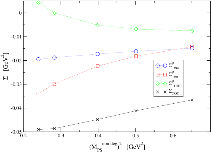
Figure 5.2: The self-energy contributions (see Eqs. 5.3, 5.4 & 5.5) versus $M_{PS}^{non-deg}$ data for the ensemble $(\beta,\kappa_{\rm sea})=(2.10,0.1382)$.

In section 5.4.3 we perform a highly constrained fit to the complete degenerate dataset. We use this method to determine an estimate of the correct value of the $\Lambda$ parameter.

5.2.1 Double Hairpin Diagrams

In eq. 5.5, $\Sigma^{\rho}_{DHP}$, the double hairpin contribution to the vector meson masses self-energy is defined. This section sketches the derivation of this term [28, 32].

The $\eta^{\prime}$ can occur as an intermediate state in the vector meson’s self-energy. However, because of the special nature of the $\eta^{\prime}$, care must be taken in order to correctly account for its propagator. In figure 5.3 the $\eta^{\prime}$ intermediate state in the vector meson’s self-energy diagram is represented. These diagrams are known as the “double hairpin (DHP) diagrams”. The left-hand diagram has no sea-quark loop insertions in the $\eta^{\prime}$ propagator, whereas the right-hand diagram has one such loop. In quenched QCD, only the left-hand diagram is present, and in full (unitary) QCD, both are present, together with diagrams including an arbitrary number of sea-quark loops. In the pseudo-quenched case, the same diagrams are allowed as in the full QCD case, except that the quarks in the loops have a mass, $m^{q}_{sea}$, which is not equal to the valence quark mass, $m^{q}_{val}$.

Concentrating on the pseudo-quenched case, the $\eta^{\prime}$ contribution to the DHP can be written as

$$\frac{-1}{(k^{2}+(M_{PS}^{deg})^{2})^{2}}\;\;\mu_{0}^{2}\;\;\bigg{(}1-\frac{\mu_{0}^{2}}{k^{2}+(M_{PS}^{unit})^{2}}+\frac{\mu_{0}^{4}}{(k^{2}+(M_{PS}^{unit})^{2})^{2}}-\ldots\bigg{)}$$ (5.7)

where $k$ is the momentum carried by the $\eta^{\prime}$, and $\mu_{0}^{2}$ is the coupling of the quark bilinears to eachother via the gluons in the sea. Note that the first term in eq. 5.7 corresponds to the case of no sea quark loop insertion (i.e. the quenched case), the second term to one sea quark loop insertion, etc.

Resumming the series in eq. 5.7 and sending $\mu_{0}\rightarrow\infty$ (since it corresponds to a mass scale which is much larger than the pion mass) gives

$$-\frac{k^{2}+(M_{PS}^{unit})^{2}}{(k^{2}+(M_{PS}^{deg})^{2})^{2}}.$$ (5.8)

There is a second diagram where the $\eta^{\prime}$ enters which involves neither a single nor double hairpin. Its contribution is

$$\frac{1}{k^{2}+(M_{PS}^{non-deg})^{2}}.$$ (5.9)

Combining eqs. 5.8 & 5.9, and rearranging gives

$$\frac{(M_{PS}^{deg})^{2}-(M_{PS}^{non-deg})^{2}}{(k^{2}+(M_{PS}^{non-deg})^{2})(k^{2}+(M_{PS}^{deg})^{2})}+\frac{(M_{PS}^{deg})^{2}-(M_{PS}^{unit})^{2}}{(k^{2}+(M_{PS}^{deg})^{2})^{2}}$$ (5.10)

which leads to the DHP self-energy term in eq. 5.5. Written in this way it is trivial to see that in the full QCD case, where $M_{PS}^{deg}\equiv M_{PS}^{non-deg}\equiv M_{PS}^{sea}$, the DHP contribution gives zero as expected, i.e. it only gives a non-zero contribution for the pseudo-quenched case.

Figure 5.3: The first of these quark flow diagrams shows the double hairpin and the second shows the double hairpin with one sea quark loop insertions. In each case the $\eta^{\prime}$ is the meson propagating along the top of the diagram.

5.3 Overview of CP-PACS Data

In [22], the CP-PACS collaboration published meson spectrum data from dynamical simulations for mean-field improved Wilson fermions with improved gluons at four different $\beta$ values. For each different $\beta$ value there are four different $\kappa_{\rm sea}$ values giving 16 independent ensembles. We summarise the lattice parameters used in table 5.1.

In figure 5.4 we plot the unitary (i.e. $\kappa_{\rm val}^{1}\equiv\kappa_{\rm val}^{2}\equiv\kappa_{\rm sea}$) pseudoscalar mass against the lattice spacing, $a_{r_{0}}$ for the 16 ensembles in table 5.1 (Note that $(M_{PS}^{unit})^{2}$ is a direct measure of the sea quark mass as outlined in section 4.9.2). Also included (for reference) are the mass values of the physical pseudo-scalar mesons $\pi,K,``\eta_{s}"$. Note the large range of both $a$ and $m^{q}_{\rm sea}$ in the simulations, and that the lattice spacing, $a$, is primarily determined by the $\beta$ value rather than the $m^{q}_{\rm sea}$ value.

The physical volume of the lattice was held fixed at $La\approx 2.5$ fm for the $\beta=1.80,1.95$ and $2.10$, but the $\beta=2.20$ ensemble had a slightly smaller physical volume. A study of finite volume effects due to this is beyond the scope of this work, and we treat all 16 ensembles on an equal footing. The mass ratio $M_{PS}/M_{V}$ is related to the mass of the sea quarks used and varies from 0.55 to 0.8. The lattice spacing $a$ varies from around 0.09 to 0.28 fm. In our study we consider the two cases where the scale is set using $r_{0}$ [21] and the string tension $\sigma$.

For each of the 16 ensembles we consider five $\kappa_{\rm val}$ values. Hence a global treatment of the data set yields a total of 80 $(M_{V}^{deg},M_{PS}^{deg})$ data points in the analysis.

We generate 1000 bootstrap clusters for all $M_{PS}$ and $M_{V}$ data using a Gaussian distribution whose central value and FWHM are the same as the central values and errors published in the table XXI of [22].

Our errors are totally uncorrelated throughout - i.e. each $M_{V}(\beta,\kappa_{\rm sea};\kappa_{\rm val}^{1},\kappa_{\rm val}^{2})$ bootstrap cluster is uncorrelated with the corresponding $M_{PS}(\beta,\kappa_{\rm sea};\kappa_{\rm val}^{1},\kappa_{\rm val}^{2})$ bootstrap cluster. Also the $M(\beta,\kappa_{\rm sea};\kappa_{\rm val}^{1},\kappa_{\rm val}^{2})$ data is uncorrelated with the $M(\beta^{\prime},\kappa_{\rm sea}^{\prime};\kappa_{\rm val}^{1},\kappa_{\rm val}^{2})$ data, and, furthermore, $M(\beta,\kappa_{\rm sea};\kappa_{\rm val}^{1},\kappa_{\rm val}^{2})$ data is uncorrelated with the $M(\beta,\kappa_{\rm sea};\kappa_{\rm val}^{1^{\prime}},\kappa_{\rm val}^{2^{\prime}})$ data.

Hence we expect the statistical errors in our final results to be overestimates of the true error because we have not benefited from any cancellation of statistical errors which should occur when combining correlated data. It is possible to estimate the increase in our errors due to the fact that we do not maintain correlations as follows. The ratio $M_{PS}^{unit}/M_{V}^{unit}$ listed in table 5.1 is obtained from our bootstrap data. Comparing this with the $M_{PS}^{unit}/M_{V}^{unit}$ data in table XXI of [22] (which benefits from the cancellation of correlations), we can see that ignoring correlations increases the errors very roughly by 20%. It is reasonable to expect a similar increase in errors for other quantities we study.

The lattice spacings $a_{r_{0},\sigma}$ are found from table XII of [22] using $r_{0}=0.49$ fm and $\sqrt{\sigma}=440$ MeV. As in the case of the meson mass data we generated 1000 bootstrap clusters with a Gaussian distribution.

The action used in [22] is tree-level, rather than non-perturbatively improved and thus is presumed to have some residual lattice systematics of ${\cal O}(a)$. We fit the data assuming both ${\cal O}(a)$ and ${\cal O}(a^{2})$ effects in sections. 5.4.2 & 5.4.3, and are thus able to obtain continuum predictions.

	$\beta$	$\kappa_{sea}$	Volume	$M_{PS}^{unit}/M_{V}^{unit}$		$a_{r_{0}}$ [fm]	$a_{\sigma}$ [fm]
	1.80	0.1409	$12^{3}\times 24$		0.8067${\scriptstyle{}^{+{9}}_{-{9}}}$	0.286${\scriptstyle{}^{+{6}}_{-{6}}}$	0.288${\scriptstyle{}^{+{3}}_{-{3}}}$
	1.80	0.1430	$12^{3}\times 24$		0.7526${\scriptstyle{}^{+{16}}_{-{15}}}$	0.272${\scriptstyle{}^{+{2}}_{-{2}}}$	0.280${\scriptstyle{}^{+{4}}_{-{5}}}$
	1.80	0.1445	$12^{3}\times 24$		0.694${\scriptstyle{}^{+{2}}_{-{2}}}$	0.258${\scriptstyle{}^{+{4}}_{-{4}}}$	0.269${\scriptstyle{}^{+{2}}_{-{3}}}$
	1.80	0.1464	$12^{3}\times 24$		0.547${\scriptstyle{}^{+{4}}_{-{4}}}$	0.237${\scriptstyle{}^{+{4}}_{-{4}}}$	0.248${\scriptstyle{}^{+{2}}_{-{3}}}$
	1.95	0.1375	$16^{3}\times 32$		0.8045${\scriptstyle{}^{+{11}}_{-{11}}}$	0.196${\scriptstyle{}^{+{4}}_{-{4}}}$	0.2044${\scriptstyle{}^{+{10}}_{-{12}}}$
	1.95	0.1390	$16^{3}\times 32$		0.752${\scriptstyle{}^{+{2}}_{-{2}}}$	0.185${\scriptstyle{}^{+{3}}_{-{3}}}$	0.1934${\scriptstyle{}^{+{14}}_{-{15}}}$
	1.95	0.1400	$16^{3}\times 32$		0.690${\scriptstyle{}^{+{2}}_{-{2}}}$	0.174${\scriptstyle{}^{+{2}}_{-{2}}}$	0.1812${\scriptstyle{}^{+{12}}_{-{12}}}$
	1.95	0.1410	$16^{3}\times 32$		0.582${\scriptstyle{}^{+{3}}_{-{3}}}$	0.163${\scriptstyle{}^{+{2}}_{-{2}}}$	0.1699${\scriptstyle{}^{+{13}}_{-{15}}}$
	2.10	0.1357	$24^{3}\times 48$		0.806${\scriptstyle{}^{+{2}}_{-{2}}}$	0.1275${\scriptstyle{}^{+{5}}_{-{5}}}$	0.1342${\scriptstyle{}^{+{8}}_{-{8}}}$
	2.10	0.1367	$24^{3}\times 48$		0.755${\scriptstyle{}^{+{2}}_{-{2}}}$	0.1203${\scriptstyle{}^{+{4}}_{-{5}}}$	0.1254${\scriptstyle{}^{+{8}}_{-{8}}}$
	2.10	0.1374	$24^{3}\times 48$		0.691${\scriptstyle{}^{+{3}}_{-{3}}}$	0.1157${\scriptstyle{}^{+{4}}_{-{4}}}$	0.1203${\scriptstyle{}^{+{6}}_{-{6}}}$
	2.10	0.1382	$24^{3}\times 48$		0.576${\scriptstyle{}^{+{3}}_{-{4}}}$	0.1093${\scriptstyle{}^{+{3}}_{-{3}}}$	0.1129${\scriptstyle{}^{+{4}}_{-{5}}}$
	2.20	0.1351	$24^{3}\times 48$		0.799${\scriptstyle{}^{+{3}}_{-{3}}}$	0.0997${\scriptstyle{}^{+{4}}_{-{5}}}$	0.10503${\scriptstyle{}^{+{15}}_{-{15}}}$
	2.20	0.1358	$24^{3}\times 48$		0.753${\scriptstyle{}^{+{4}}_{-{4}}}$	0.0966${\scriptstyle{}^{+{4}}_{-{4}}}$	0.1013${\scriptstyle{}^{+{3}}_{-{2}}}$
	2.20	0.1363	$24^{3}\times 48$		0.705${\scriptstyle{}^{+{6}}_{-{6}}}$	0.0936${\scriptstyle{}^{+{4}}_{-{4}}}$	0.0978${\scriptstyle{}^{+{3}}_{-{3}}}$
	2.20	0.1368	$24^{3}\times 48$		0.632${\scriptstyle{}^{+{8}}_{-{8}}}$	0.0906${\scriptstyle{}^{+{4}}_{-{4}}}$	0.0949${\scriptstyle{}^{+{2}}_{-{2}}}$

Table 5.1: The lattice parameters of the CP-PACS simulation used in this data analysis taken from[22]. The superscript unit refers to the unitary data, i.e. where $\kappa_{\rm val}^{1}\equiv\kappa_{\rm val}^{2}\equiv\kappa_{\rm sea}$. Note that the errors reported in this table are obtained with our bootstrap ensembles (see sec.5.4.1).

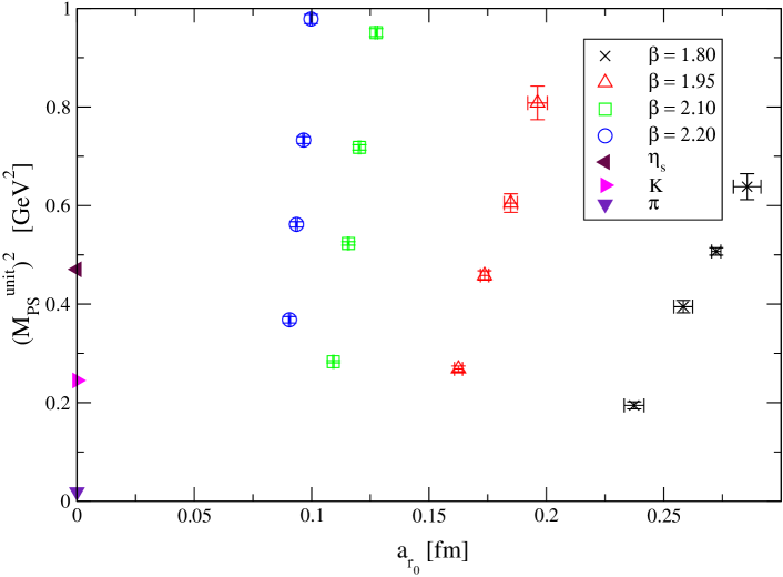
Figure 5.4: A plot showing the range of sea quark mass $(M_{PS}^{unit})^{2}$ and lattice spacing, $a_{r_{0}}$), covered by the CP-PACS data as displayed in Table 5.1. $(M_{PS}^{unit})^{2}$ is the pseudo-scalar meson mass squared at the unitary point, i.e. where $\kappa_{\rm val}\equiv\kappa_{\rm sea}$). The experimental points for the $\pi,K$ and “$\eta_{s}$” mesons are also shown for reference.

5.4 Fitting Analysis

5.4.1 Summary of Analysis Techniques

Our method is centred on converting all masses into physical units prior to performing any extrapolations. An alternative to this would be to extrapolate dimensionless masses (i.e. values in lattice units) as in [22]. We believe that our method has the following advantages:

• We can combine the data from different ensembles and treat it in a global manner. If we left the masses in dimensionless units, we could not combine data from different ensembles due to differing lattice spacings.

• Dimensionful mass predictions from lattice simulations are effectively mass ratios, and so we expect some of the systematic (and statistical) errors to cancel, e.g. $M^{dimful}=M^{\#}\times a^{-1}\equiv M^{\#}/M_{\Omega}^{\#}\times M_{\Omega}^{expt}$ where $\Omega$ is the quantity used to set the lattice spacing, $a$, the superscripts #, $expt$ refer to the dimensionless lattice mass estimate and experimental value respectively.

We consider two different methods for setting the scale. These are determining the lattice spacing from the string tension $(\sigma)$ and from the Sommer scale $(r_{0})$. We find one method is better than the other. This is outlined in section 5.4.3. Table 5.1 lists values for $a_{r_{0}}$ and $a_{\sigma}$. We also consider the effects of using other quantities to set the scale.

We compare the Adelaide method with a naive polynomial fit. Our fitting functions take the following form, for the Adelaide fits

$$\sqrt{(M_{V}^{deg})^{2}-\Sigma_{TOT}} = a_{0}+a_{2}(M_{PS}^{deg})^{2}+a_{4}(M_{PS}^{deg})^{4}+a_{6}(M_{PS}^{deg})^{6}$$ (5.11)

where $\Sigma_{TOT}$ is from Eq.(5.2), and for the naive polynomial fit

$$\hskip 42.67912ptM_{V}^{deg}=a_{0}+a_{2}(M_{PS}^{deg})^{2}+a_{4}(M_{PS}^{deg})^{4}+a_{6}(M_{PS}^{deg})^{6}$$ (5.12)

We divide these fits into two further subcategories. The first category includes the above fits and is referred to as “cubic” since they include cubic terms in the chiral expansion of $m^{q}_{\rm sea}\propto(M_{PS}^{deg})^{2}$. The second category is formed from fits with the coefficient $a_{6}$ set to zero in equations 5.11 & 5.12. We call this category “quadratic”.

We note that the dominant functional form of $M_{V}$ with $(M_{PS}^{deg})^{2}$ is linear for example see figure 5.5. This fact is exploited in the above fitting functions. This is why the Adelaide fit uses $\sqrt{(M_{V}^{deg})^{2}-\Sigma_{TOT}}$ on the left hand side rather than $(M_{V}^{deg})^{2}-\Sigma_{TOT}$ which would be an equally valid chiral expansion. It follows for the above argument that we can expect the $a_{n}$ coefficients to be small for $n>4$, and this is in fact what we find. In the following subsection we fit to equations 5.11 & 5.12 for the 16 ensembles in Table 5.1 separately. We then consider a holistic approach where we combine the data from all 16 ensembles and perform a single global fit.

5.4.2 Individual ensemble fits

We first consider an individual analysis of the meson spectrum. This is done by treating the 16 ensembles listed in table 5.1 separately. We perform fits to the five $(M_{V}^{deg},M_{PS}^{deg})$ data points available from each ensemble. The fitting functions used are the Adelaide (eq. 5.11) and the naive (eq. 5.12) fitting functions. We restrict our attention to quadratic ($a_{6}\equiv 0$) chiral fits because there are only five data points available for each analysis. We use $r_{0}$ to set the scale and the $\Lambda$ parameter for the Adelaide fits is set to $\Lambda=650$ [MeV] which is our preferred value (see Sec.5.4.3).

The results for the coefficients $a_{0,2,4}$ which are obtained by fitting $M_{V}$ against $M_{PS}$ using both the naive (eq. 5.12) and Adelaide (eq. 5.11) fitting functions are listed in table 5.2. The fact that the $a_{4}$ coefficients are small and in most cases poorly determined supports our decision to fit to the quadratic, rather than the cubic chiral extrapolation form.

Another important point to note is that there is a level of agreement between the naive and Adelaide $a_{0,2}$ coefficients, although their variation with $\kappa_{\rm sea}$ tends to be different.

	$\beta$	$\kappa_{sea}$	$a^{naive}_{0}$	$a^{adel}_{0}$	$a^{naive}_{2}$	$a^{adel}_{2}$	$a^{naive}_{4}$	$a^{adel}_{4}$
			[GeV]	[GeV]	[GeV-1]	[GeV-1]	[GeV-3]	[GeV-3]
	1.80	0.1409	0.701${\scriptstyle{}^{+{14}}_{-{22}}}$	0.70${\scriptstyle{}^{+{2}}_{-{2}}}$	0.46${\scriptstyle{}^{+{7}}_{-{3}}}$	0.54${\scriptstyle{}^{+{5}}_{-{5}}}$	-0.01${\scriptstyle{}^{+{3}}_{-{7}}}$	-0.09${\scriptstyle{}^{+{5}}_{-{5}}}$
	1.80	0.1430	0.712${\scriptstyle{}^{+{14}}_{-{13}}}$	0.724${\scriptstyle{}^{+{14}}_{-{13}}}$	0.48${\scriptstyle{}^{+{6}}_{-{6}}}$	0.51${\scriptstyle{}^{+{5}}_{-{6}}}$	-0.04${\scriptstyle{}^{+{6}}_{-{6}}}$	-0.08${\scriptstyle{}^{+{6}}_{-{6}}}$
	1.80	0.1445	0.73${\scriptstyle{}^{+{2}}_{-{2}}}$	0.756${\scriptstyle{}^{+{14}}_{-{15}}}$	0.43${\scriptstyle{}^{+{5}}_{-{5}}}$	0.44${\scriptstyle{}^{+{5}}_{-{5}}}$	0.01${\scriptstyle{}^{+{5}}_{-{5}}}$	-0.01${\scriptstyle{}^{+{5}}_{-{5}}}$
	1.80	0.1464	0.72${\scriptstyle{}^{+{2}}_{-{2}}}$	0.769${\scriptstyle{}^{+{13}}_{-{15}}}$	0.49${\scriptstyle{}^{+{5}}_{-{5}}}$	0.43${\scriptstyle{}^{+{5}}_{-{5}}}$	-0.02${\scriptstyle{}^{+{6}}_{-{6}}}$	0.007${\scriptstyle{}^{+{59}}_{-{58}}}$
	1.95	0.1375	0.76${\scriptstyle{}^{+{2}}_{-{2}}}$	0.75${\scriptstyle{}^{+{2}}_{-{2}}}$	0.49${\scriptstyle{}^{+{4}}_{-{4}}}$	0.53${\scriptstyle{}^{+{4}}_{-{4}}}$	-0.05${\scriptstyle{}^{+{4}}_{-{3}}}$	-0.08${\scriptstyle{}^{+{3}}_{-{3}}}$
	1.95	0.1390	0.76${\scriptstyle{}^{+{2}}_{-{2}}}$	0.772${\scriptstyle{}^{+{17}}_{-{15}}}$	0.47${\scriptstyle{}^{+{4}}_{-{4}}}$	0.49${\scriptstyle{}^{+{4}}_{-{4}}}$	-0.03${\scriptstyle{}^{+{4}}_{-{3}}}$	-0.05${\scriptstyle{}^{+{4}}_{-{4}}}$
	1.95	0.1400	0.785${\scriptstyle{}^{+{12}}_{-{12}}}$	0.803${\scriptstyle{}^{+{11}}_{-{11}}}$	0.43${\scriptstyle{}^{+{4}}_{-{4}}}$	0.44${\scriptstyle{}^{+{4}}_{-{4}}}$	-0.01${\scriptstyle{}^{+{3}}_{-{3}}}$	-0.02${\scriptstyle{}^{+{3}}_{-{3}}}$
	1.95	0.1410	0.766${\scriptstyle{}^{+{13}}_{-{15}}}$	0.799${\scriptstyle{}^{+{13}}_{-{14}}}$	0.48${\scriptstyle{}^{+{5}}_{-{4}}}$	0.45${\scriptstyle{}^{+{5}}_{-{4}}}$	-0.03${\scriptstyle{}^{+{4}}_{-{4}}}$	-0.03${\scriptstyle{}^{+{3}}_{-{4}}}$
	2.10	0.1357	0.829${\scriptstyle{}^{+{14}}_{-{14}}}$	0.820${\scriptstyle{}^{+{14}}_{-{14}}}$	0.42${\scriptstyle{}^{+{5}}_{-{4}}}$	0.46${\scriptstyle{}^{+{5}}_{-{4}}}$	-0.02${\scriptstyle{}^{+{3}}_{-{4}}}$	-0.05${\scriptstyle{}^{+{3}}_{-{4}}}$
	2.10	0.1367	0.794${\scriptstyle{}^{+{11}}_{-{10}}}$	0.797${\scriptstyle{}^{+{11}}_{-{10}}}$	0.50${\scriptstyle{}^{+{3}}_{-{3}}}$	0.53${\scriptstyle{}^{+{3}}_{-{3}}}$	-0.06${\scriptstyle{}^{+{3}}_{-{3}}}$	-0.08${\scriptstyle{}^{+{3}}_{-{2}}}$
	2.10	0.1374	0.807${\scriptstyle{}^{+{13}}_{-{14}}}$	0.822${\scriptstyle{}^{+{13}}_{-{14}}}$	0.48${\scriptstyle{}^{+{4}}_{-{4}}}$	0.49${\scriptstyle{}^{+{4}}_{-{4}}}$	-0.05${\scriptstyle{}^{+{3}}_{-{3}}}$	-0.06${\scriptstyle{}^{+{3}}_{-{3}}}$
	2.10	0.1382	0.781${\scriptstyle{}^{+{10}}_{-{9}}}$	0.814${\scriptstyle{}^{+{10}}_{-{9}}}$	0.53${\scriptstyle{}^{+{3}}_{-{3}}}$	0.50${\scriptstyle{}^{+{3}}_{-{3}}}$	-0.08${\scriptstyle{}^{+{2}}_{-{2}}}$	-0.07${\scriptstyle{}^{+{2}}_{-{2}}}$
	2.20	0.1351	0.84${\scriptstyle{}^{+{3}}_{-{3}}}$	0.84${\scriptstyle{}^{+{3}}_{-{3}}}$	0.43${\scriptstyle{}^{+{8}}_{-{8}}}$	0.46${\scriptstyle{}^{+{8}}_{-{8}}}$	-0.02${\scriptstyle{}^{+{6}}_{-{6}}}$	-0.04${\scriptstyle{}^{+{6}}_{-{6}}}$
	2.20	0.1358	0.83${\scriptstyle{}^{+{2}}_{-{2}}}$	0.84${\scriptstyle{}^{+{2}}_{-{2}}}$	0.44${\scriptstyle{}^{+{7}}_{-{7}}}$	0.46${\scriptstyle{}^{+{7}}_{-{7}}}$	-0.03${\scriptstyle{}^{+{5}}_{-{5}}}$	-0.05${\scriptstyle{}^{+{5}}_{-{5}}}$
	2.20	0.1363	0.80${\scriptstyle{}^{+{3}}_{-{3}}}$	0.81${\scriptstyle{}^{+{3}}_{-{3}}}$	0.51${\scriptstyle{}^{+{8}}_{-{8}}}$	0.52${\scriptstyle{}^{+{8}}_{-{8}}}$	-0.07${\scriptstyle{}^{+{6}}_{-{6}}}$	-0.08${\scriptstyle{}^{+{6}}_{-{6}}}$
	2.20	0.1368	0.78${\scriptstyle{}^{+{2}}_{-{2}}}$	0.80${\scriptstyle{}^{+{2}}_{-{2}}}$	0.52${\scriptstyle{}^{+{8}}_{-{8}}}$	0.51${\scriptstyle{}^{+{7}}_{-{8}}}$	-0.06${\scriptstyle{}^{+{6}}_{-{6}}}$	-0.06${\scriptstyle{}^{+{6}}_{-{6}}}$

Table 5.2: The coefficients obtained from fitting $M_{V}$ data against $M_{PS}^{2}$ using both the naive and Adelaide fits (i.e. eqs.(5.12 & 5.11)) for each of the 16 ensembles listed in Table 5.1. As discussed in the text we restrict these fits to quadratic rather than cubic chiral functions (i.e. $a_{6}\equiv 0$). The scale was set from $r_{0}$.

We give a representative example of these fits in figure 5.5 using the ensemble $(\beta,\kappa_{\rm sea})=(2.10,0.1382)$. This ensemble’s $(a,m^{q}_{\rm sea})$ coordinates are closest to the physical point $(a,m^{q}_{\rm sea})=(0,m_{u,d})$ for ensembles with $La\approx 2.5\,$[fm] (see fig.5.4).

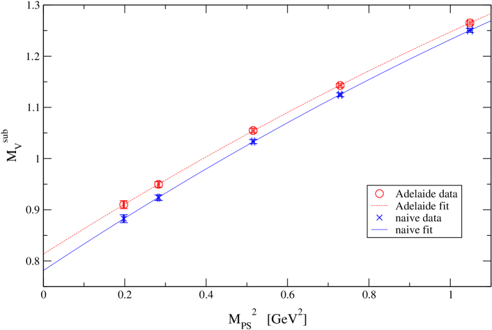
Figure 5.5: A plot of $M_{V}^{Sub}$ versus $M_{PS}$ data for the ensemble $(\beta,\kappa_{\rm sea})=(2.10,0.1382)$ together with the results of the quadratic Adelaide (Eq.5.11) and naive (Eq.5.12) fits. $M_{V}^{Sub}$ is defined as $M_{V}^{Sub}=\sqrt{(M_{V}^{deg})^{2}-\Sigma_{TOT}}$ for the Adelaide fit (i.e. the L.H.S. of Eq.5.11 - note $\Sigma_{TOT}$ is negative).

In figures 5.6 & 5.7 we investigate the correlation of the $(a_{0},a_{2})$ coefficients for both the Adelaide and naive fits. As expected, as $a_{0}$ increases, $a_{2}$ decreases. Both methods show this trend to some extent. The figures also indicate that there might be a systematic variation of $a_{0,2}$ with $a_{r_{0}}$. To investigate this further we plot $a_{0}$ and $a_{2}$ against $a_{r_{0}}$ (for both the linear and Adelaide fits) in figures 5.8 & 5.9. We use these figures to motivate a continuum extrapolation of the form

$$a_{0,2}=a_{0,2}^{cont}+X^{individual}_{0,2}\;a_{r_{0}}$$ (5.13)

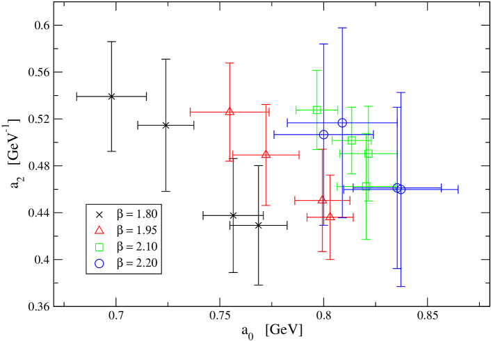
Figure 5.6: A scatter plot of $a_{2}$ against $a_{0}$ for the Adelaide fit showing their mutual correlation.

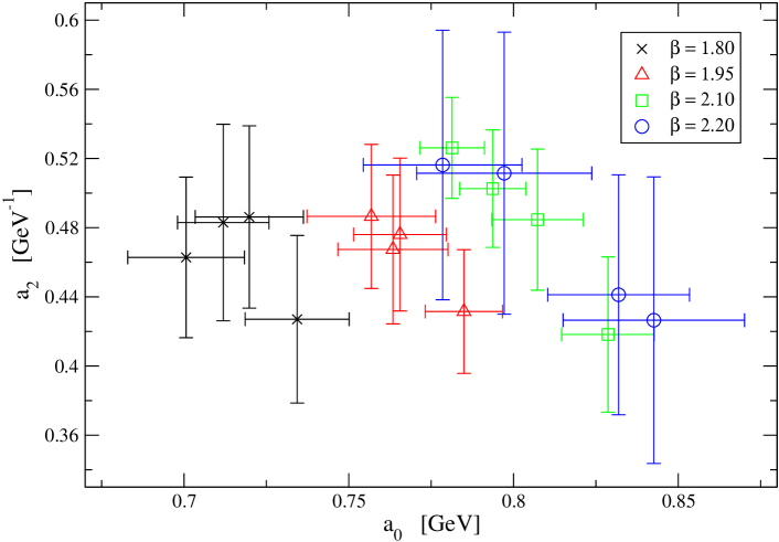
Figure 5.7: A scatter plot of $a_{2}$ against $a_{0}$ for the naive fit showing their mutual correlation.

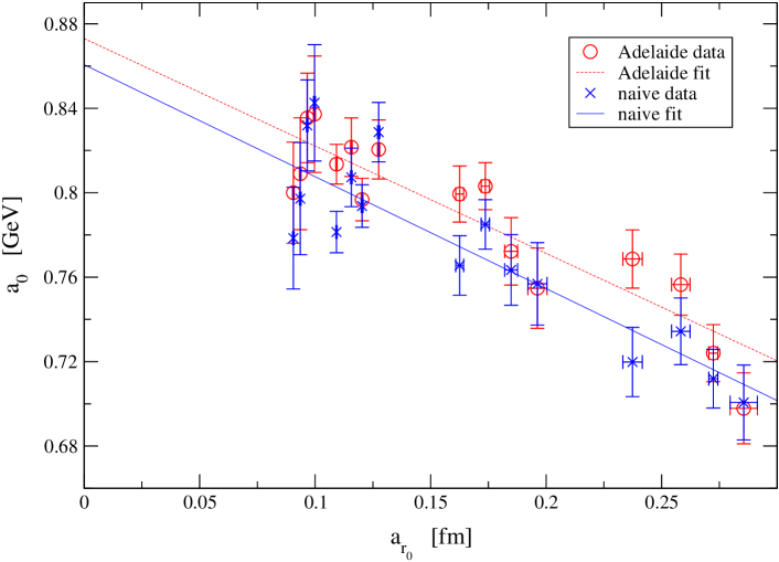
Figure 5.8: A continuum extrapolation of the $a_{0}$ coefficient obtained from both the Adelaide and naive fits Eq.(5.13).

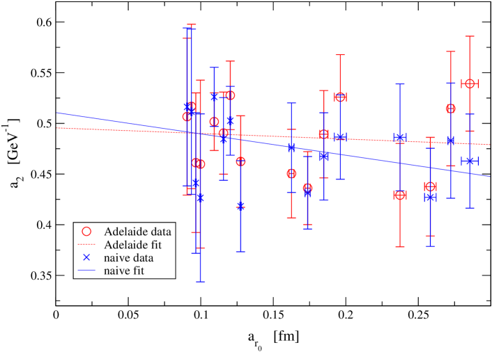
Figure 5.9: A continuum extrapolation of the $a_{2}$ coefficient obtained from both the Adelaide and naive fits Eq.(5.13).

We list the results of these fits in table 5.3.

The values of $X^{individual}_{0,2}$ in table 5.3 confirms a statistically significant ${\cal O}(a)$ effect in the $a_{0}$ coefficient but is absent from the $a_{2}$ coefficient. (Note we could have also performed a fit which involves for example a ${\cal O}(a^{2})$ term. We investigate these fitting forms in more detail in the following section.)

	$a_{0}^{cont.}$	$X^{individual}_{0}$	$\chi^{2}_{0}/d.o.f.$	$a_{2}^{cont.}$	$X^{individual}_{2}$	$\chi^{2}_{2}/d.o.f.$
	[GeV]	[GeV/fm]		[GeV-1]	[GeV-1/fm]
Naive-fit	0.861${\scriptstyle{}^{+{11}}_{-{9}}}$	-0.53${\scriptstyle{}^{+{5}}_{-{7}}}$	21 / 14	0.51${\scriptstyle{}^{+{3}}_{-{4}}}$	-0.21${\scriptstyle{}^{+{23}}_{-{15}}}$	8 / 14
Adelaide-fit	0.873${\scriptstyle{}^{+{10}}_{-{10}}}$	-0.51${\scriptstyle{}^{+{5}}_{-{6}}}$	16 / 14	0.50${\scriptstyle{}^{+{3}}_{-{3}}}$	-0.06${\scriptstyle{}^{+{19}}_{-{18}}}$	10 / 14

Table 5.3: The coefficients obtained from the continuum extrapolation of both the naive and Adelaide $a_{0,2}$ values from Table 5.2 using eq.(5.13).

We now investigate the possibility of the lattice meson spectrum having a sea quark dependency. This is done by plotting the coefficients $a_{0,2}-X^{individual}_{0,2}a_{r_{0}}$ against $(1/M_{PS}^{unit})^{2}$. The results of this are shown in figures 5.10 & 5.11. (Recall the superscript unit refers to the unitary data $\kappa_{\rm val}^{1}\equiv\kappa_{\rm val}^{2}\equiv\kappa_{\rm sea}$.) This is done because from the usual PCAC relation, $(M_{PS}^{unit})^{2}\propto m^{q}_{\rm sea}$. We chose to plot $(1/M_{PS}^{unit})^{2}$ as the $x-$coordinate rather than $(M_{PS}^{unit})^{2}$ because this allows us to plot the quenched point at $(1/M_{PS}^{unit})^{2}\equiv 0$ rather than at infinity. It should be pointed out that the physical point corresponds to $(1/M_{PS}^{unit})^{2}\sim 50$, consequently it is some way from our data. We subtract $X^{individual}_{0,2}a_{r_{0}}$ in the $y-$coordinate of figures 5.10 & 5.11 in a hope that we will be left with the residual $m^{q}_{\rm sea}$ effects. This is done because, as we have seen, variations in lattice spacing dominate those in $m^{q}_{\rm sea}$.

Figures 5.10 & 5.11 show that there are little if any significant $m^{q}_{\rm sea}$ dependencies in $a_{0,2}$. Moreover linear fits to $(1/M_{PS}^{unit})^{2}$ produces a gradient which is almost zero within errors for the $a_{2}$ term. We conclude this subsection by noting that we have not observed any evidence of unquenching effects in the the data.

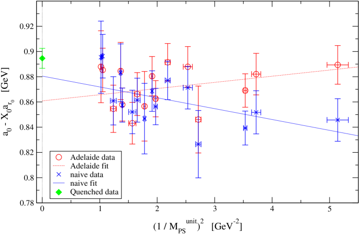
Figure 5.10: A chiral extrapolation of the $a_{0}-X^{individual}_{0}a$ coefficient obtained from both the linear and Adelaide fits. Also plotted is the quenched data point, see sec. 5.4.4. The scale was taken from $r_{0}$.

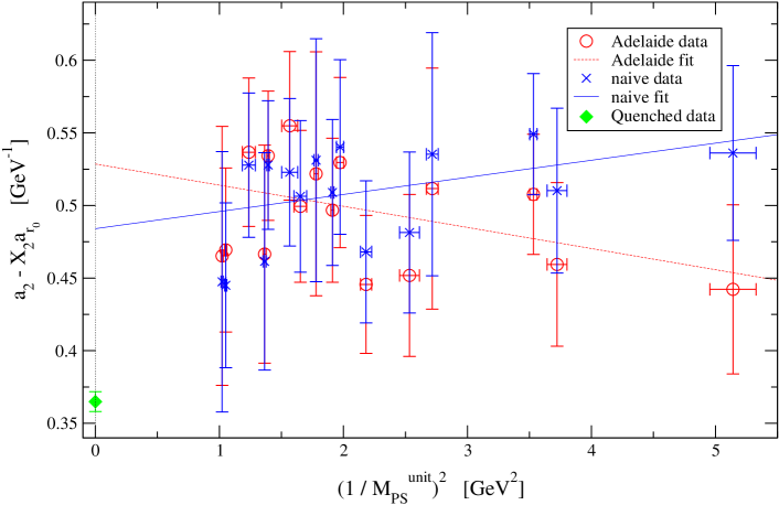
Figure 5.11: A chiral extrapolation of the $a_{2}-X^{individual}_{2}a$ coefficient obtained from both the linear and Adelaide fits. Also plotted is the quenched data point, see sec. 5.4.4. The scale was taken from $r_{0}$.

5.4.3 Global fits

In this section we treat the degenerate data from the 16 different ensembles as a whole data set. Doing this produces a data set containing 80 points (16 ensembles with five $(M_{V}^{deg},M_{PS}^{deg})$ values in each). Our hope is that this larger data set will constrain the fits allowing us to fit to more complicated functional forms and also produce a highly constrained set of fit parameters $a_{0,2,\ldots}$. Figure 5.12 is a graphical representation of the $80$ degenerate CP-PACS data points where we have set the scale from $r_{0}$.

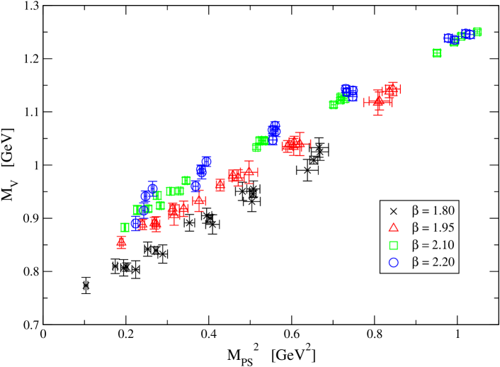
Figure 5.12: A plot of the degenerate CP-PACS data set. We have set the scale using a${}_{r_{0}}$.

If we are to treat the data as a whole data set it is very important to model the lattice artefacts correctly. Table 5.2 along with the discussion in the previous section indicates a variation amongst the $a_{0}$ values with lattice spacing, but the $a_{2}$ coefficient is approximately constant with lattice spacing. Also recall that the $a_{4}$ coefficient was undetermined. Hence we believe that allowing for variation in the $a_{0}$ coefficient due to the lattice spacing will be sufficient to correct any significant lattice artifacts.

We use the above to motivate the following fitting functions. We define a modified version of the Adelaide and naive fitting function based on equations 5.11 & 5.12.

$$\sqrt{(M_{V}^{deg})^{2}-\Sigma_{TOT}} = (a_{0}^{cont}+X_{1}a+X_{2}a^{2})+a_{2}(M_{PS}^{deg})^{2}$$ (5.14)

$$+a_{4}(M_{PS}^{deg})^{4}+a_{6}(M_{PS}^{deg})^{6}$$

$$M_{V}^{deg} = (a_{0}^{cont}+X_{1}a+X_{2}a^{2})+a_{2}(M_{PS}^{deg})^{2}$$ (5.15)

$$+a_{4}(M_{PS}^{deg})^{4}+a_{6}(M_{PS}^{deg})^{6}$$

As in the individual analysis (sec 5.4.2) we refer to the above fits as “cubic”, since they include the $a_{6}$ term $\propto m_{q}^{3}$. As above we also perform fits with $a_{6}$ set to zero, referring to these as “quadratic”.

We include corrections for ${\cal O}(a)$ and ${\cal O}(a^{2})$ lattice spacing effects in the fitting functions 5.14 & 5.15. This is because the lattice action used is tree-level improved, and so we expect it to contain ${\cal O}(a^{2})$ errors, but as shown in section 5.4.2 there is also some residual ${\cal O}(a)$ errors.

We have studied fitting functions that include ${\cal O}(a,a^{2})$ terms in the $a_{2}$ (and even $a_{4}$) coefficients to try to uncover lattice spacing effects in the higher order coefficients but we have found that these fits are unstable. This confirms the findings of our individual analysis reinforcing our belief that the discernible lattice spacing effects are contained in the $a_{0}$ coefficient.

In this section we study two different methods for setting the scale. We use both the Sommer scale $(r_{0})$ and the string tension, $(\sigma)$. We summarise these different fits in table 5.4. In total we study $2^{4}$ fitting procedures, any one of these fitting procedures can be built by moving from left to right across table 5.4 and making a choice from the available options in each column.

Approach	Chiral Extrapolation	Treatment of Lattice	Lattice Spacing
		Spacing Artefact’s in $a_{0}$	set from
Adelaide	Cubic	$a_{0}$ term has	$r_{0}$
i.e. eq.5.14	i.e. ${\cal O}(M_{PS}^{6})$ included	${\cal O}(a+a^{2})$ corrections
Naive	Quadratic	$a_{0}$ term has	$\sigma$
i.e. eq.5.15	i.e. no ${\cal O}(M_{PS}^{6})$ term	only ${\cal O}(a^{2})$ corrections

Table 5.4: The different fit types used in the global analysis. Fits for each of the $2^{4}$ choices depicted above were performed.

We expect these fits to be highly constrained since they are performed using a data set containing 80 data points and the largest number of free parameters studied is six ($a_{0},X_{1},X_{2},a_{2},a_{4}$ and $a_{6}$).

When performing the Adelaide fits we must determine the correct value of the $\Lambda$ parameter (sec 5.2). This parameter is introduced in the Adelaide approach to model the size of the quasi-particle under consideration. It is this length scale that controls the chiral physics. Although it is not possible to allow $\Lambda$ to be a free parameter in our fits we can derive the best value for $\Lambda$ as follows. We manually vary the value of $\Lambda$ and then plot the $\chi^{2}/d.o.f.$ as a function of $\Lambda$. Figure 5.13 is a graphical representation of this. When the scale is set from $r_{0}$ the $\chi^{2}$ value as a function of $\Lambda$ exhibits the same functional form for all fits and they share a distinct minimum at $\Lambda\approx 650$ [MeV]. Explicitly this means that the $\Lambda$ parameter has no dependence on the order of the chiral expansion of our fits (i.e. expanding to ${\cal O}(M_{PS}^{4})$ or ${\cal O}(M_{PS}^{6})$ has no effect on the correct value of $\Lambda$) also there is no dependence on our modelling of the lattice systematics in the $a_{0}$ coefficient (i.e. we can choose to use either ${\cal O}(a+a^{2})$ or ${\cal O}(a^{2})$).

When the scale is set using the string tension $(\sigma)$ figure 5.13 again shows that the $\chi^{2}$ all exhibit the same functional form. Now though we see that all fits share a distinct minimum at $\Lambda\approx 550$ [MeV]. The discrepancy in the correct value of $\Lambda$ which arises when using different methods to set the scale will be addressed in section 5.5.1. However we see that now the ${\cal O}(a+a^{2})$ fits give a far better $\chi^{2}$ that the ${\cal O}(a^{2})$ fits. To investigate this further we have fitted the data using a fitting function with only ${\cal O}(a)$ correction in the $a_{0}$ coefficient (i.e. eq. 5.14 with $X_{2}=0$). The results showed near identical $\chi^{2}$ values as for the ${\cal O}(a+a^{2})$ fits. This is indicative of a dominant ${\cal O}(a)$ lattice-spacing systematic in the cases where the string tension is used to set the scale. We offer no explanation why this should be the case.

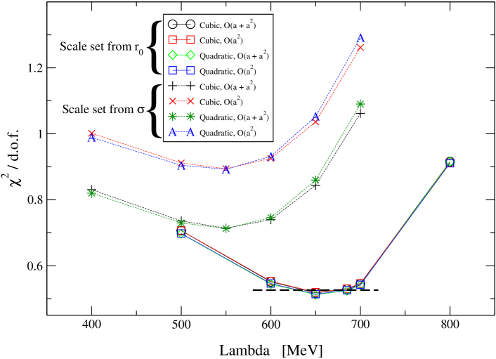
Figure 5.13: A plot of $\chi^{2}/d.o.f$ against $\Lambda$. The dashed horizontal line represents increasing $\chi^{2}$ from its minimum value by unity for the $r_{0}$ data (i.e. it represents one standard deviation), see sec. 5.5. The intercept of this dashed line with the $\chi^{2}$ curves (at $\Lambda=$630 and 690 MeV) is used to derive upper and lower bounds for the preferred $\Lambda$ value.

These preferred values of $\Lambda$ (550 [MeV] & 650 [MeV] for the a_σ and a${}_{r_{0}}$ cases respectively) are used to perform the 16 global fits that are outlined in table 5.4. We list the results of these different fits along with the $\chi^{2}/d.o.f.$ in table 5.5.

Fit	Scale	$a_{0}^{cont}$	$X_{1}$	$X_{2}$	$a_{2}$	$a_{4}$	$a_{6}$	$\chi^{2}/d.o.f.$
Approach	from	[GeV]	[GeVfm-1]	[GeVfm-2]	[GeV-1]	[GeV-3]	[GeV-5]
Cubic chiral extrapolation        $a_{0}$ contains ${\cal O}(a+a^{2})$
Adelaide	$r_{0}$	0.844${\scriptstyle{}^{+{13}}_{-{16}}}$	-0.11${\scriptstyle{}^{+{15}}_{-{13}}}$	-1.1${\scriptstyle{}^{+{3}}_{-{4}}}$	0.47${\scriptstyle{}^{+{5}}_{-{4}}}$	-0.02${\scriptstyle{}^{+{8}}_{-{10}}}$	-0.02${\scriptstyle{}^{+{5}}_{-{4}}}$	38 / 74
Adelaide	$\sigma$	0.836${\scriptstyle{}^{+{9}}_{-{11}}}$	-0.37${\scriptstyle{}^{+{10}}_{-{9}}}$	-0.2${\scriptstyle{}^{+{2}}_{-{3}}}$	0.44${\scriptstyle{}^{+{5}}_{-{4}}}$	0.04${\scriptstyle{}^{+{7}}_{-{9}}}$	-0.06${\scriptstyle{}^{+{5}}_{-{4}}}$	53 / 74
Naive	$r_{0}$	0.819${\scriptstyle{}^{+{13}}_{-{17}}}$	-0.15${\scriptstyle{}^{+{15}}_{-{13}}}$	-1.1${\scriptstyle{}^{+{3}}_{-{4}}}$	0.56${\scriptstyle{}^{+{6}}_{-{5}}}$	-0.16${\scriptstyle{}^{+{8}}_{-{10}}}$	0.05${\scriptstyle{}^{+{5}}_{-{4}}}$	77 / 74
Naive	$\sigma$	0.805${\scriptstyle{}^{+{10}}_{-{12}}}$	-0.38${\scriptstyle{}^{+{11}}_{-{9}}}$	-0.3${\scriptstyle{}^{+{2}}_{-{3}}}$	0.57${\scriptstyle{}^{+{5}}_{-{4}}}$	-0.18${\scriptstyle{}^{+{8}}_{-{10}}}$	0.06${\scriptstyle{}^{+{6}}_{-{5}}}$	73 / 74
Cubic chiral extrapolation        $a_{0}$ contains ${\cal O}(a^{2})$ only
Adelaide	$r_{0}$	0.835${\scriptstyle{}^{+{8}}_{-{9}}}$	-	-1.40${\scriptstyle{}^{+{3}}_{-{4}}}$	0.48${\scriptstyle{}^{+{5}}_{-{4}}}$	-0.03${\scriptstyle{}^{+{8}}_{-{10}}}$	-0.02${\scriptstyle{}^{+{5}}_{-{4}}}$	39 / 75
Adelaide	$\sigma$	0.807${\scriptstyle{}^{+{6}}_{-{8}}}$	-	-1.24${\scriptstyle{}^{+{3}}_{-{3}}}$	0.43${\scriptstyle{}^{+{5}}_{-{4}}}$	0.06${\scriptstyle{}^{+{8}}_{-{9}}}$	-0.06${\scriptstyle{}^{+{5}}_{-{4}}}$	67 / 75
Naive	$r_{0}$	0.806${\scriptstyle{}^{+{8}}_{-{10}}}$	-	-1.49${\scriptstyle{}^{+{4}}_{-{4}}}$	0.56${\scriptstyle{}^{+{6}}_{-{5}}}$	-0.17${\scriptstyle{}^{+{8}}_{-{10}}}$	0.06${\scriptstyle{}^{+{5}}_{-{4}}}$	78 / 75
Naive	$\sigma$	0.775${\scriptstyle{}^{+{7}}_{-{8}}}$	-	-1.31${\scriptstyle{}^{+{4}}_{-{4}}}$	0.56${\scriptstyle{}^{+{5}}_{-{4}}}$	-0.16${\scriptstyle{}^{+{8}}_{-{10}}}$	0.05${\scriptstyle{}^{+{5}}_{-{5}}}$	87 / 75
Quadratic chiral extrapolation        $a_{0}$ contains ${\cal O}(a+a^{2})$
Adelaide	$r_{0}$	0.840${\scriptstyle{}^{+{10}}_{-{12}}}$	-0.11${\scriptstyle{}^{+{14}}_{-{13}}}$	-1.1${\scriptstyle{}^{+{3}}_{-{4}}}$	0.493${\scriptstyle{}^{+{12}}_{-{11}}}$	-0.061${\scriptstyle{}^{+{8}}_{-{9}}}$	-	38 / 75
Adelaide	$\sigma$	0.829${\scriptstyle{}^{+{8}}_{-{9}}}$	-0.37${\scriptstyle{}^{+{10}}_{-{9}}}$	-0.2${\scriptstyle{}^{+{2}}_{-{3}}}$	0.490${\scriptstyle{}^{+{13}}_{-{11}}}$	-0.052${\scriptstyle{}^{+{10}}_{-{11}}}$	-	54 / 75
Naive	$r_{0}$	0.828${\scriptstyle{}^{+{11}}_{-{13}}}$	-0.16${\scriptstyle{}^{+{15}}_{-{13}}}$	-1.1${\scriptstyle{}^{+{3}}_{-{4}}}$	0.505${\scriptstyle{}^{+{13}}_{-{11}}}$	-0.068${\scriptstyle{}^{+{9}}_{-{10}}}$	-	78 / 75
Naive	$\sigma$	0.812${\scriptstyle{}^{+{8}}_{-{9}}}$	-0.37${\scriptstyle{}^{+{11}}_{-{9}}}$	-0.3${\scriptstyle{}^{+{2}}_{-{3}}}$	0.523${\scriptstyle{}^{+{13}}_{-{12}}}$	-0.075${\scriptstyle{}^{+{11}}_{-{11}}}$	-	74 / 75
Quadratic chiral extrapolation        $a_{0}$ contains ${\cal O}(a^{2})$ only
Adelaide	$r_{0}$	0.832${\scriptstyle{}^{+{4}}_{-{4}}}$	-	-1.40${\scriptstyle{}^{+{3}}_{-{4}}}$	0.494${\scriptstyle{}^{+{12}}_{-{11}}}$	-0.061${\scriptstyle{}^{+{8}}_{-{9}}}$	-	39 / 76
Adelaide	$\sigma$	0.799${\scriptstyle{}^{+{3}}_{-{4}}}$	-	-1.23${\scriptstyle{}^{+{3}}_{-{3}}}$	0.486${\scriptstyle{}^{+{13}}_{-{11}}}$	-0.046${\scriptstyle{}^{+{10}}_{-{11}}}$	-	68 / 76
Naive	$r_{0}$	0.815${\scriptstyle{}^{+{4}}_{-{4}}}$	-	-1.49${\scriptstyle{}^{+{4}}_{-{4}}}$	0.506${\scriptstyle{}^{+{12}}_{-{11}}}$	-0.068${\scriptstyle{}^{+{8}}_{-{10}}}$	-	79 / 76
Naive	$\sigma$	0.781${\scriptstyle{}^{+{3}}_{-{4}}}$	-	-1.31${\scriptstyle{}^{+{3}}_{-{4}}}$	0.520${\scriptstyle{}^{+{13}}_{-{12}}}$	-0.069${\scriptstyle{}^{+{11}}_{-{11}}}$	-	88 / 76

Table 5.5: The results of the global fit analysis. Fits for all $2^{4}$ fit combinations depicted in table 5.4 are shown.

We now summarise the results of these of these fits (tb 5.5 and fig 5.13).

• Fit approach
  The smallest $\chi^{2}/d.o.f.$ (and hence the best fit) is given by the Adelaide method. Moreover we see consistently smaller $\chi^{2}$ for a given fit using the Adelaide method compared to the corresponding fit derived from our naive approach. This confirms that the Adelaide approach is the preferred chiral extrapolation procedure.

• Chiral extrapolation
  In all cases the cubic chiral extrapolation (i.e. including a ${\cal O}(M_{PS}^{6})$ term) leads to a undetermined $a_{6}$ coefficient. We also observe the $a_{4}$ coefficient in the cubic fits becomes poorly determined compared to its quadratic chiral extrapolation counterpart.

• Treatment of the lattice spacing systematics
  Studying the coefficients $a_{0}$ and $a_{2}$ in table 5.5, we see that in the case where $r_{0}$ is used to set the scale, the coefficients have little dependence on the type of lattice spacing correction used (i.e whether ${\cal O}(a+a^{2})$ or ${\cal O}(a^{2})$ is used in the $a_{0}$ coefficient). We do see a reduction in the error of the $a_{0}$ coefficient when only a ${\cal O}(a^{2})$ correction is used, this is most likely due to reducing the number of degrees of freedom. When the scale is set using $\sigma$, we see that this is no longer true and that the coefficients $a_{0}$ and $a_{2}$ do depend on the treatment of the lattice spacing systematics. This supports the conjecture that setting the scale using the string tension leads to ${\cal O}(a)$ systematics.

• Setting the scale
  We see that in the Adelaide approach the $\chi^{2}$ is drastically reduced compared to when $\sigma$ is used to set the scale (fig 5.13). This along with the discussion regarding probable ${\cal O}(a)$ systematics in the $\sigma$ data, give us reason to favour setting the scale using $r_{0}$. In the case of the naive fits there is no clear preference between setting the scale from either $r_{0}$ or $\sigma$.

Using the above to guide our choice we select the quadratic chiral extrapolation method with ${\cal O}(a^{2})$ corrections in the $a_{0}$ coefficient where the scale is set from $r_{0}$ to define the central value of both the Adelaide and naive fitting procedure. The spread from the other fitting types is used to define the error. We make predictions for physical meson masses in section 5.5 for these fitting types.

5.4.4 Quenched data.

Along with the dynamical case, we have studied quenched data from [22]. This data was produced from simulations that use the same (gauge) lattice action as the dynamical case. We use values listed in table XIII of [22] for the string tension and $r_{0}$ to determine the lattice spacing where we take $r_{0}=0.49$ [fm] and $\sqrt{\sigma}=440$ [MeV].

As in our dynamical analysis we represent the quenched data in [22] by a Gaussian distribution of 1000 bootstrap samples. We ensure the distribution has its mean equal to central value of the original data and its FWHM is equal to the error of the original data in [22]. Table 5.6 gives an overview of the parameters of these simulations.

	$\beta$	Volume	$a_{r_{0}}$	$a_{0}^{r_{0}}$	$a_{2}^{r_{0}}$	$a_{\sigma}$	$a_{0}^{\sigma}$	$a_{2}^{\sigma}$
			[fm]	[GeV]	[GeV-1]	[fm]	[GeV]	[GeV-1]
	2.187	$16^{3}$ $\times$ 32	0.196${\scriptstyle{}^{+{3}}_{-{3}}}$	0.777${\scriptstyle{}^{+{12}}_{-{14}}}$	0.421${\scriptstyle{}^{+{10}}_{-{10}}}$	0.2083${\scriptstyle{}^{+{15}}_{-{15}}}$	0.733${\scriptstyle{}^{+{8}}_{-{10}}}$	0.446${\scriptstyle{}^{+{9}}_{-{9}}}$
	2.214	$16^{3}$ $\times$ 32	0.187${\scriptstyle{}^{+{3}}_{-{3}}}$	0.776${\scriptstyle{}^{+{14}}_{-{17}}}$	0.423${\scriptstyle{}^{+{12}}_{-{11}}}$	0.1980${\scriptstyle{}^{+{12}}_{-{13}}}$	0.732${\scriptstyle{}^{+{8}}_{-{9}}}$	0.448${\scriptstyle{}^{+{10}}_{-{10}}}$
	2.247	$16^{3}$ $\times$ 32	0.175${\scriptstyle{}^{+{2}}_{-{2}}}$	0.787${\scriptstyle{}^{+{12}}_{-{12}}}$	0.426${\scriptstyle{}^{+{10}}_{-{12}}}$	0.1856${\scriptstyle{}^{+{9}}_{-{10}}}$	0.742${\scriptstyle{}^{+{8}}_{-{9}}}$	0.452${\scriptstyle{}^{+{10}}_{-{11}}}$
	2.281	$16^{3}$ $\times$ 32	0.163${\scriptstyle{}^{+{2}}_{-{2}}}$	0.824${\scriptstyle{}^{+{14}}_{-{13}}}$	0.391${\scriptstyle{}^{+{11}}_{-{11}}}$	0.1729${\scriptstyle{}^{+{10}}_{-{9}}}$	0.778${\scriptstyle{}^{+{10}}_{-{10}}}$	0.415${\scriptstyle{}^{+{11}}_{-{11}}}$
	2.334	$16^{3}$ $\times$ 32	0.1490${\scriptstyle{}^{+{9}}_{-{10}}}$	0.835${\scriptstyle{}^{+{10}}_{-{10}}}$	0.387${\scriptstyle{}^{+{9}}_{-{9}}}$	0.1580${\scriptstyle{}^{+{9}}_{-{9}}}$	0.787${\scriptstyle{}^{+{9}}_{-{9}}}$	0.411${\scriptstyle{}^{+{9}}_{-{9}}}$
	2.416	$24^{3}$ $\times$ 48	0.1281${\scriptstyle{}^{+{5}}_{-{4}}}$	0.860${\scriptstyle{}^{+{10}}_{-{12}}}$	0.371${\scriptstyle{}^{+{11}}_{-{10}}}$	0.1361${\scriptstyle{}^{+{8}}_{-{7}}}$	0.810${\scriptstyle{}^{+{10}}_{-{11}}}$	0.394${\scriptstyle{}^{+{12}}_{-{11}}}$
	2.456	$24^{3}$ $\times$ 48	0.1201${\scriptstyle{}^{+{5}}_{-{5}}}$	0.843${\scriptstyle{}^{+{8}}_{-{8}}}$	0.394${\scriptstyle{}^{+{8}}_{-{8}}}$	0.1268${\scriptstyle{}^{+{13}}_{-{13}}}$	0.798${\scriptstyle{}^{+{11}}_{-{10}}}$	0.416${\scriptstyle{}^{+{9}}_{-{9}}}$
	2.487	$24^{3}$ $\times$ 48	0.1143${\scriptstyle{}^{+{4}}_{-{4}}}$	0.855${\scriptstyle{}^{+{10}}_{-{9}}}$	0.384${\scriptstyle{}^{+{10}}_{-{9}}}$	0.1208${\scriptstyle{}^{+{9}}_{-{9}}}$	0.810${\scriptstyle{}^{+{11}}_{-{10}}}$	0.405${\scriptstyle{}^{+{11}}_{-{10}}}$
	2.528	$24^{3}$ $\times$ 48	0.1072${\scriptstyle{}^{+{4}}_{-{5}}}$	0.857${\scriptstyle{}^{+{10}}_{-{10}}}$	0.385${\scriptstyle{}^{+{8}}_{-{9}}}$	0.1132${\scriptstyle{}^{+{9}}_{-{11}}}$	0.812${\scriptstyle{}^{+{11}}_{-{10}}}$	0.406${\scriptstyle{}^{+{9}}_{-{10}}}$
	2.575	$24^{3}$ $\times$ 48	0.1003${\scriptstyle{}^{+{3}}_{-{3}}}$	0.859${\scriptstyle{}^{+{9}}_{-{9}}}$	0.385${\scriptstyle{}^{+{8}}_{-{8}}}$	0.106${\scriptstyle{}^{+{6}}_{-{7}}}$	0.81${\scriptstyle{}^{+{6}}_{-{5}}}$	0.41${\scriptstyle{}^{+{3}}_{-{3}}}$

Table 5.6: The lattice parameters of the quenched CP-PACS simulation used in this data analysis [22] together with the results of a linear chiral extrapolation. Note that the errors reported in this table are obtained with our bootstrap ensembles (see sec.5.4.1).

In [22] the quenched data was fitted with a linear fitting function of the following form (see eq.(59) and table XIV of [22])

$$aM_{V}=A^{V}+B^{V}(aM_{PS})^{2}.$$ (5.16)

This linear chiral fit is a simplified version of our naive fitting functions. It contains no $a_{4}$ or $a_{6}$ coefficients (hence is linear in $m_{q}^{sea}$). To analyse this data we use the values of the coefficients $A^{V}$ and $B^{V}$ (table XIV of [22]) of the fits performed in [22]. We do this because no individual masses for the quenched data are published. We convert these coefficients into dimensionful values via $a_{0}=A^{V}/a$ and $a_{2}=B^{V}a$. We study both cases where the scale is set using $r_{0}$ and the string tension. Table 5.6 lists the resulting dimensionful $a_{0,2}$ coefficients.

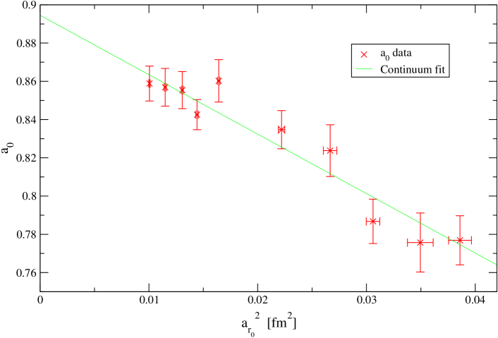
Figure 5.14: An ${\cal O}(a^{2})$ continuum extrapolation of the quenched $a_{0}$ coefficients (i.e. using eq.(5.17) with $X^{(0)}_{1}=0$). $r_{0}$ was used to set the scale.

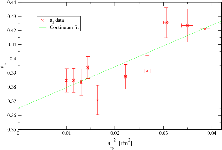
Figure 5.15: An ${\cal O}(a^{2})$ continuum extrapolation of the quenched $a_{2}$ coefficients (i.e. using eq.(5.17) with $X^{(2)}_{1}=0$). $r_{0}$ was used to set the scale.

We investigate the dependency of these coefficients on lattice spacing by plotting the coefficients $a_{0}$ and $a_{2}$ against lattice spacing $a$. Figures 5.14 and 5.15 represent the case where the scale is set from $r_{0}$. We see a clear lattice spacing dependency for the $a_{0}$ coefficient; the $a_{2}$ coefficient also appears to exhibit a dependency on the lattice spacing. We model the lattice spacing artefacts by assuming the same two $a-$dependencies in $a_{0,2}$ as in sec. 5.4.3

$$a_{(0,2)}=a_{(0,2)}^{cont}+X^{(0,2)}_{1}a+X^{(0,2)}_{2}a^{2}.$$ (5.17)

We perform the above ${\cal O}(a+a^{2})$ continuum extrapolation, along with an ${\cal O}(a^{2})$ extrapolation (i.e. we set $X^{(0,2)}_{1}=0$ in eq 5.17). We choose an ${\cal O}(a^{2})$ extrapolation rather than ${\cal O}(a)$ because we expect the action to be dominated by ${\cal O}(a^{2})$ lattice spacing artifacts. Hence a linear extrapolation in the lattice spacing (achieved by setting $X^{(0,2)}_{2}=0$ in eq 5.17) would not be appropriate. Our results from these fits show that the ${\cal O}(a+a^{2})$ fit leads to poorly determined coefficients $X^{(0,2)}_{1,2}$. A point of inflection can also be seen in the fit which is located between the data and the continuum point $(a=0)$.

We list our results for the values of $a_{0,2}^{cont}$ and $X^{(0,2)}_{2}$ from the ${\cal O}(a^{2})$ extrapolations in table 5.7. Graphically these fits are depicted in figures 5.14 and 5.15. The fact that the $X^{(0,2)}_{2}$ coefficients are significantly different from zero provide clear evidence for lattice spacing effects in the $a_{0,2}$ coefficients for the quenched case. The continuum values, $a_{0,2}^{cont}$, are plotted in figs. 5.10 & 5.11 and are surprisingly consistent with the dynamical data.

In the following section we produce continuum estimates for the masses of the vector meson spectrum. We use these quenched values of $a_{0,2}^{cont}$ to include estimates of continuum quenched values of the vector meson spectrum

	$a_{0}^{cont.}$	$X^{(0)}_{2}$	$\chi^{2}_{0}/d.o.f$	$a_{2}^{cont.}$	$X^{(2)}_{2}$	$\chi^{2}_{2}/d.o.f$
	[GeV]	[GeV/fm]		[GeV-1]	[GeV-1/fm]
From $a_{r_{0}}$	0.895${\scriptstyle{}^{+{8}}_{-{7}}}$	-3.1${\scriptstyle{}^{+{3}}_{-{4}}}$	6.7 / 8	0.365${\scriptstyle{}^{+{6}}_{-{7}}}$	1.5${\scriptstyle{}^{+{3}}_{-{3}}}$	9.9 / 8
From $a_{\sigma}$	0.853${\scriptstyle{}^{+{9}}_{-{8}}}$	-2.9${\scriptstyle{}^{+{3}}_{-{3}}}$	6.6 / 8	0.381${\scriptstyle{}^{+{8}}_{-{9}}}$	1.6${\scriptstyle{}^{+{3}}_{-{3}}}$	9.3 / 8

Table 5.7: The coefficients obtained from performing a continuum extrapolation (eq. 5.17) to the $a_{0,2}$ quenched coefficients. (Note we have set $X^{(0,2)}_{1}\equiv 0$ – see text.)

5.5 Physical Predictions

In this section we make physical predictions for the continuum masses of the $\rho,~{}K^{\ast}~{}\&~{}\phi$ $(M_{\rho},M_{K^{\ast}}$ & $M_{\phi})$. We do this for both the Adelaide and naive methods (eqs 5.11 & 5.12) that have previously been explored (sec 5.4.3).

All mass predictions in this section are produced using our global fitting method rather than the individual analysis introduced in section 5.4.2. We choose the global method because we expect the coefficients produced to be more accurate than those from section 5.4.2 since the global fits are highly constrained.

In this section we also study the $M_{\rho}$ prediction as a function of $\Lambda$. We choose to study the variation of the $\rho$-mass because it will be more sensitive to a changing value of $\Lambda$ because $\Sigma_{TOT}$ is largest for smallest meson mass.

The mass predictions for $M_{\rho},M_{K^{\ast}}$ & $M_{\phi}$ are obtained by setting $M_{PS}^{non-deg}$, $M_{PS}^{deg}~{}\&~{}M_{PS}^{unit}$ in equations 5.11 & 5.12 to the values outlined in table 5.8.

Vector Meson	$M_{PS}^{deg}$	$M_{PS}^{non-deg}$	$M_{PS}^{unit}$
$\rho$	$\mu_{\pi}$	$\mu_{\pi}$	$\mu_{\pi}$
$K^{\ast}$	$\mu_{K}$	$\mu_{K}/\sqrt{2}$	$\mu_{\pi}$
$\phi$	$\mu_{\eta_{s}}$	$\mu_{K}$	$\mu_{\pi}$

Table 5.8: Values for $M_{PS}^{deg},M_{PS}^{non-deg}$ and $M_{PS}^{unit}$ used in equations 5.2 - 5.5, 5.11, 5.12 to calculate estimates of M_ρ, M${}_{K^{\ast}}$ and M_ϕ. The symbol $\mu$ is used to represent the physical masses of the mesons. Note that the values for $M_{PS}^{non-deg}$ are obtained by recalling that the non-degenerate meson contains one “valence” and one sea quark and that $M_{PS}^{2}\propto m_{q}$.

We assume an $SU(3)$ flavour symmetry and so we expect the $K$ and $K^{\ast}$ mesons to have valence quarks with a mass equal to half that of the strange quark. To calculate the self energy terms in the continuum a fourth order Runge-Kutta method is employed to calculate the integrals. We set $M_{PS}^{unit}$ to $M_{\pi}$ throughout (because a unitary meson will comprise two sea quarks) and we assume that $\Delta M_{\omega\rho}=0$. Physical predictions are made using all of the $2^{4}$ fitting types that were discussed in section 5.4.3 (table 5.4). To do this the coefficients, $a_{0}^{cont}\&a_{2,4,6}$, from these fits (i.e. those in table 5.5), are used. We also make a prediction for the quenched vector meson spectrum as discussed in the previous section. Here we use the coefficients from section 5.4.4 listed in table 5.6. For all of the above cases we study both methods of setting the scale, using $r_{0}$ and the string tension.

We list results for all of our mass predictions in table 5.9. We have used our preferred values of $\Lambda$, $\Lambda=650(550)$ [MeV] (for the cases when the scale is set from $r_{0}(\sigma)$ respectively).

Figure 5.16 graphically represents our investigations into how the $M_{\rho}$ prediction varies with the value of $\Lambda$ for each of the eight Adelaide fits. To estimate an acceptable range for the $\Lambda$ parameter we use the $\chi^{2}$ plot of section 5.4.3 (figure 5.13). Using this plot we can estimate the range of acceptable $\Lambda$ values defined by increasing $\chi^{2}$ by unity from its minimum, this represents one standard deviation.

The horizontal dashed line in figure 5.13 lies along $\chi^{2}$ values which are increased by one standard deviation (for our preferred method of setting the scale i.e the $r_{0}$ case). Hence we find that an acceptable range of values for $\Lambda$ lies between 630 [MeV] $\leq\Lambda\leq$ 690 [MeV].

We represent this range in figure 5.16 by plotting two vertical dashed lines at the acceptable maximum and minimum values of $\Lambda$.

Source	Fit	Scale	Mρ	MK∗	Mϕ	Jdiscrete
	Procedure	from	[GeV]	[GeV]	[GeV]
Experiment			0.770	0.892	1.0194	0.487
Quenched	Naive	$r_{0}$	0.902${\scriptstyle{}^{+{8}}_{-{7}}}$	0.984${\scriptstyle{}^{+{8}}_{-{7}}}$	1.066${\scriptstyle{}^{+{8}}_{-{7}}}$	0.359${\scriptstyle{}^{+{7}}_{-{8}}}$
”	Naive	$\sigma$	0.861${\scriptstyle{}^{+{9}}_{-{8}}}$	0.947${\scriptstyle{}^{+{9}}_{-{8}}}$	1.033${\scriptstyle{}^{+{9}}_{-{8}}}$	0.361${\scriptstyle{}^{+{9}}_{-{9}}}$
	Cubic chiral extrapolation        $a_{0}$ contains ${\cal O}(a+a^{2})$
Dynamical	Adelaide	$r_{0}$	0.792${\scriptstyle{}^{+{12}}_{-{16}}}$	0.889${\scriptstyle{}^{+{11}}_{-{13}}}$	1.029${\scriptstyle{}^{+{11}}_{-{12}}}$	0.38${\scriptstyle{}^{+{3}}_{-{3}}}$
”	Adelaide	$\sigma$	0.810${\scriptstyle{}^{+{9}}_{-{11}}}$	0.886${\scriptstyle{}^{+{8}}_{-{9}}}$	1.026${\scriptstyle{}^{+{8}}_{-{9}}}$	0.29${\scriptstyle{}^{+{3}}_{-{2}}}$
”	Naive	$r_{0}$	0.829${\scriptstyle{}^{+{12}}_{-{16}}}$	0.947${\scriptstyle{}^{+{11}}_{-{12}}}$	1.051${\scriptstyle{}^{+{10}}_{-{12}}}$	0.49${\scriptstyle{}^{+{3}}_{-{3}}}$
”	Naive	$\sigma$	0.815${\scriptstyle{}^{+{9}}_{-{12}}}$	0.936${\scriptstyle{}^{+{8}}_{-{9}}}$	1.042${\scriptstyle{}^{+{8}}_{-{9}}}$	0.50${\scriptstyle{}^{+{3}}_{-{2}}}$
	Cubic chiral extrapolation        $a_{0}$ contains ${\cal O}(a^{2})$ only
Dynamical	Adelaide	$r_{0}$	0.782${\scriptstyle{}^{+{7}}_{-{9}}}$	0.879${\scriptstyle{}^{+{2}}_{-{2}}}$	1.0198${\scriptstyle{}^{+{18}}_{-{15}}}$	0.38${\scriptstyle{}^{+{3}}_{-{2}}}$
”	Adelaide	$\sigma$	0.781${\scriptstyle{}^{+{6}}_{-{7}}}$	0.853${\scriptstyle{}^{+{2}}_{-{2}}}$	0.9946${\scriptstyle{}^{+{18}}_{-{14}}}$	0.27${\scriptstyle{}^{+{3}}_{-{2}}}$
”	Naive	$r_{0}$	0.817${\scriptstyle{}^{+{7}}_{-{9}}}$	0.935${\scriptstyle{}^{+{2}}_{-{2}}}$	1.039${\scriptstyle{}^{+{2}}_{-{2}}}$	0.49${\scriptstyle{}^{+{3}}_{-{3}}}$
”	Naive	$\sigma$	0.786${\scriptstyle{}^{+{6}}_{-{7}}}$	0.905${\scriptstyle{}^{+{2}}_{-{2}}}$	1.0109${\scriptstyle{}^{+{18}}_{-{15}}}$	0.48${\scriptstyle{}^{+{3}}_{-{2}}}$
	Quadratic chiral extrapolation        $a_{0}$ contains ${\cal O}(a+a^{2})$
Dynamical	Adelaide	$r_{0}$	0.789${\scriptstyle{}^{+{11}}_{-{13}}}$	0.889${\scriptstyle{}^{+{11}}_{-{13}}}$	1.029${\scriptstyle{}^{+{11}}_{-{12}}}$	0.392${\scriptstyle{}^{+{10}}_{-{9}}}$
”	Adelaide	$\sigma$	0.805${\scriptstyle{}^{+{8}}_{-{9}}}$	0.886${\scriptstyle{}^{+{8}}_{-{9}}}$	1.026${\scriptstyle{}^{+{8}}_{-{9}}}$	0.316${\scriptstyle{}^{+{10}}_{-{9}}}$
”	Naive	$r_{0}$	0.837${\scriptstyle{}^{+{11}}_{-{13}}}$	0.948${\scriptstyle{}^{+{10}}_{-{13}}}$	1.051${\scriptstyle{}^{+{10}}_{-{12}}}$	0.462${\scriptstyle{}^{+{11}}_{-{10}}}$
”	Naive	$\sigma$	0.822${\scriptstyle{}^{+{8}}_{-{9}}}$	0.935${\scriptstyle{}^{+{8}}_{-{9}}}$	1.041${\scriptstyle{}^{+{8}}_{-{9}}}$	0.471${\scriptstyle{}^{+{10}}_{-{10}}}$
	Quadratic chiral extrapolation        $a_{0}$ contains ${\cal O}(a^{2})$ only
Dynamical	Adelaide	$r_{0}$	0.779${\scriptstyle{}^{+{4}}_{-{4}}}$	0.879${\scriptstyle{}^{+{2}}_{-{2}}}$	1.0200${\scriptstyle{}^{+{16}}_{-{14}}}$	0.389${\scriptstyle{}^{+{9}}_{-{8}}}$
”	Adelaide	$\sigma$	0.774${\scriptstyle{}^{+{3}}_{-{3}}}$	0.853${\scriptstyle{}^{+{2}}_{-{2}}}$	0.9950${\scriptstyle{}^{+{16}}_{-{14}}}$	0.299${\scriptstyle{}^{+{8}}_{-{7}}}$
”	Naive	$r_{0}$	0.825${\scriptstyle{}^{+{4}}_{-{4}}}$	0.935${\scriptstyle{}^{+{2}}_{-{2}}}$	1.0381${\scriptstyle{}^{+{16}}_{-{14}}}$	0.456${\scriptstyle{}^{+{9}}_{-{8}}}$
”	Naive	$\sigma$	0.791${\scriptstyle{}^{+{3}}_{-{3}}}$	0.905${\scriptstyle{}^{+{2}}_{-{2}}}$	1.0106${\scriptstyle{}^{+{17}}_{-{14}}}$	0.453${\scriptstyle{}^{+{9}}_{-{8}}}$

Table 5.9: Estimates of M_ρ, M${}_{K^{\ast}}$, M_ϕ and J obtained from the global fits.

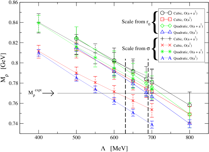
Figure 5.16: A plot of $M_{\rho}$ as a function of $\Lambda$ from the Adelaide approach. Recall that the best $\Lambda$ value when the scale is set from $r_{0}(\sigma)$ is $\Lambda=650(550)$ MeV. The two vertical dashed lines define the range of acceptable $\Lambda$ values (630 MeV $\leq\Lambda\leq$ 690 MeV) obtained by increasing $\chi^{2}$ by unity in fig. 5.13.

We summarise the information in table 5.9 and figure 5.16 below.

• The statistical errors in the mass estimates are typically about 1%.

• We see disagreement in the Adelaide fits when we choose to set the scale using different methods. The Adelaide procedure is very stable when we set the scale using $r_{0}$. But when setting the scale using the string tension, we see that the four Adelaide fits do not agree and so appear to be unstable. We believe that this is most likely due to there being residual ${\cal O}(a)$ errors when the scale is set using the string tension (sec 5.4.3).

• The results obtained from the Adelaide fitting procedure are very accurate. At most they are twice the statistical standard error from the experimental value. For the Adelaide method to reproduce exactly the experimental $M_{\rho}$ value, a re-adjustment of only around 1-2% in $r_{0}$, and around 2-6% in $\sqrt{\sigma}$ would be required.

• Notice (fig 5.16) that the variation of $M_{\rho}$ with $\Lambda$ is very small, it is about the same order as the other uncertainties.

• The Adelaide method has central values that are far closer to the experimental values than the naive method has. Furthermore the naive fitting method has larger spread of values than the Adelaide procedure.

• The quenched results significantly overestimate $M_{\rho}$. The quenched value of the $J$-parameter is also significantly underestimated. (These two facts mean that the $M_{\phi}$ quenched prediction is more accurate than the $M_{\rho}$ value.)

All of these points are in favour of the Adelaide method. Consequently we believe that the Adelaide method should be the favoured method when performing chiral extrapolations and we note that Adelaide method is a significant improvement over the naive approach.

To give a final value for $M_{\rho}$ for both the Adelaide method and the naive method, we use our preferred fitting function (the quadratic fit with ${\cal O}(a^{2})$ corrections in the $a_{0}$ coefficient) and our preferred method for setting the scale (from $r_{0}$). Our error for the different fitting methods is obtained from the spread in the mass predictions (for the $r_{0}$ case). We also include an estimate of the error associated with the $\Lambda$ parameter. We determine this by varying $\chi^{2}$ by unity (as described above). We can then simply read off this error from the vertical dashed lines in figure 5.16.

Hence Our final estimates are:

$$M_{\rho}^{Adelaide} = 779(4){\scriptstyle{}^{+{13}}_{-{0}}}{\scriptstyle{}^{+{5}}_{-{10}}}\textrm{[MeV]}$$ (5.18)

$$M_{\rho}^{Naive} = 825(4){\scriptstyle{}^{+{12}}_{-{8}}}\textrm{[MeV]}$$ (5.19)

where the first error is statistical and the second is from the fit procedure. In the Adelaide case the third error is that associated with $\Lambda$. We do not make explicit any error that is associated with the determination of $r_{0}$.

We finally include a study of the $J$–parameter. This is normally defined as [21]

$$J=M_{V}\frac{dM_{V}}{dM_{PS}^{2}}\bigg{\arrowvert}_{K,K^{\ast}}$$ (5.21)

Here though we study the “discrete” version of this which we define as

$$J^{discrete}=M_{K*}\left(\frac{M_{K*}-M_{\rho}}{M_{K}^{2}-M_{\pi}^{2}}\right)$$ (5.22)

We use this discrete version of $J$ $(J^{discrete})$ because it can be easily determined from experimental data, but $J$ itself cannot. These two definitions coincide if $M_{V}$ is a strict linear function of $M_{PS}^{2}$.

Table 5.9 lists values for $J^{discrete}$. We see that the value of $J^{discrete}$ is a severe underestimate of the experimental value. This is a well known phenomena and is no surprise. We also note that the estimates of $J^{discrete}$ for the dynamical cases do increase toward the experimental value.

5.5.1 Setting the lattice spacing

In this section we investigate the differences in our results that occur when setting the scale using different methods. As previously mentioned we have studied two methods used for setting the scale. These are from the Sommer scale $(r_{0})$ and from the string tension $(\sigma)$. We investigate the ratio of these scales by plotting $a_{\sigma}/a_{r_{0}}$ against $r_{0}$ for each of the 16 ensembles in table 5.1. We see that this ratio is almost constant for the 16 ensembles and that there is almost no evidence of ${\cal O}(a)$ or $m_{q}$ dependencies. The ratio is always greater than one and a rough estimate of its value would be around $5\%$ above unity. We believe that this can be explained if the product $\sqrt{\sigma}r_{0}=440$ MeV $\times~{}0.49$ [fm] is approximately 5 % below its real value. It is this that presumably explains why, when setting the scale using $r_{0}$, the estimates of the vector meson mass are larger than those found from using the string tension. Since the Adelaide method has a highly non-linear relationship between the lattice scale $(a^{-1})$, and estimates of the vector meson mass $(M_{V})$ due to the self energy $(\Sigma_{TOT})$ there is no corresponding simple relationship for the estimates of the vector meson mass made using different methods to set the scale.

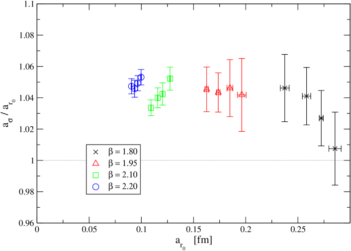
Figure 5.17: A plot showing the ratio $a_{\sigma}/a_{r_{0}}$ against $a_{r_{0}}$ for the ensembles in table 5.1.

This non-unit ratio must be responsible for the difference in the predicted best value of $\Lambda$ that can be observed when using different methods to set the scale (fig. 5.17). It follows therefore if $a_{\sigma}/a_{r_{0}}$ were unity, then we would see identical Adelaide predictions when using $r_{0}$ and $\sigma$ to set the scale.

We also investigate one final method for setting the scale. This is the method of [25]. This method fixes the lattice spacing (and the strange quark mass) from the $(K,K^{\ast})$ mass point, i.e. using the $J$-parameter. The results of this method are graphically represented in figure 5.18. As in our global analysis we plot the full degenerate CP-PACS data set (80 degenerate points from [22]). Figure 5.18 also includes the unitary UKQCD points from [26]. It is quite remarkable that when this method is used, our data lies on an almost universal straight line. Compare this with the case where $r_{0}$ is used to set the scale (fig. 5.12) and note that this is exactly the same data set.

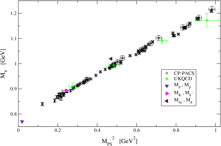
Figure 5.18: The vector meson masses, $M_{V}$ versus $M_{PS}^{2}$ from the CP-PACS collaboration [22]. The scale is set from the $(K,K^{\ast})$ point using the method in [25]. Also shown are the unitary UKQCD points from [26].

The method of [25] seems to be an ideal way of setting the scale since the data would be well modelled by a simple linear fit. This is because the data is forced to go through the $(M_{K},M_{K^{\ast}})$ point, leaving the gradient as the only free parameter. But in doing this we are normalising away the expected non-linear behaviour as the chiral limit is approached, and it is exactly this behaviour that we try to describe using the self-energy term $\Sigma_{TOT}$ in eq. . It is for this reason that we believe, despite the universal behaviour of the data when the scale is set using the $J$-parameter (fig. 5.12), it would be incorrect to use this method to set the scale in this work.

5.6 Conclusions

We conclude this chapter by listing the results of our study.

• We have shown that the Adelaide method is a valid chiral extrapolation procedure and we have generalised the Adelaide chiral ansatz to “pseudo-quenched” case (i.e. when $\kappa_{\rm sea}\neq\kappa_{\rm val}$).

• We have quantified the residual ${\cal O}(a)$ effects in the CP-PACS data. (See e.g. figs.5.8 & 5.9.)

• We have studied different fitting methods and found our global procedure to be the better method.

• We have demonstrated that the Adelaide method can predict a preferred value for the $\Lambda$ parameter.

• We have indicated that small errors in the values of $r_{0}$ and $\sigma$ might be the cause of the slight inaccuracy in the central values of our mass estimates.

• We have obtained estimates of the $\rho$, $K^{*}$ & $\phi$ masses with tiny (statistical) error bars. (See table 5.9.)

• We have estimated systematic errors in the $\rho$ mass from the fitting procedure (both chiral and continuum fitting procedure).

Note that we have not modelled finite-size effects - see Sec. 5.3. This is because we do not have enough different volumes to undertake such a study. Finite volume effects are considered by the Adelaide method (eq 5.6) since the momentum integral is replaced by the appropriate kinetic sum.

Chapter 6 An analysis of the Nucleon mass from lattice QCD

.

6.1 Introduction

In this chapter we again use the chiral extrapolation technique developed by the Adelaide group to estimate the mass of the nucleon from lattice QCD. We will employ a dipole form factor as we did in chapter 5 and we will also study a Gaussian form factor in an attempt to prove that the Adelaide method is not dependent on the finite-range regulator that is employed. In the next section we list the finite-range regulator form for the self-energy of the nucleon in the pseudo-quenched case. We again use the data generated by the CP-PACS group in [22]. We provided a comprehensive review of this data in 5.3 for the $\rho$ case and also, for the nucleon data, in 6.3. In section 6.4 we outline the various fitting methods that we employ. Section 6.4.4 investigates the differences between the Gaussian and dipole finite-range regulators. The section following this contains our physical predictions for the nucleon mass. We then discuss the different methods of setting the scale. Finally in section 6.7 we draw our conclusions.

6.2 The partially quenched ansatz

In this analysis we restrict our attention to the case where the valence quarks are degenerate ($\kappa_{\rm val}^{1}=\kappa_{\rm val}^{2}=\kappa_{\rm val}^{3}=\kappa_{\rm val}$).

We begin by defining the following shorthand notation

$$\begin{array}[]{rcl}M_{B}^{non\_deg}&=&M_{PS}(\beta,\kappa_{\rm sea};\kappa_{\rm sea},\kappa_{\rm val},\kappa_{\rm val})\\ M_{B}^{deg}&=&M_{PS}(\beta,\kappa_{\rm sea};\kappa_{\rm val},\kappa_{\rm val},\kappa_{\rm val})\\ M_{PS}^{non\_deg}&=&M_{PS}(\beta,\kappa_{\rm sea};\kappa_{\rm sea},\kappa_{\rm val})\\ M_{PS}^{deg}&=&M_{PS}(\beta,\kappa_{\rm sea};\kappa_{\rm val},\kappa_{\rm val})\\ M_{PS}^{unit}&=&M_{PS}(\beta,\kappa_{\rm sea};\kappa_{\rm sea},\kappa_{\rm sea})\end{array}$$ (6.6)

where $M_{B(PS)}$ is the Baryon(pseudo-scalar) mass with $B=N~{}\&~{}\Delta$. The first two arguments of $M_{B(PS)}$ refer to the sea structure (i.e. the gauge coupling and sea quark hopping parameter) and the last three(two) arguments refer to the valence quark hopping parameters.

We also define the following integrals

$$I(M_{PS},\delta M) = \frac{2}{\pi}\int_{0}^{\infty}\frac{k^{4}u^{2}(k)dk}{\omega(\omega+\delta M)}$$

$$I_{2}(M_{PS}) = \frac{2}{\pi}\int_{0}^{\infty}\frac{k^{4}u^{2}(k)dk}{\omega^{4}}$$ (6.7)

Where we have used:

$$\omega(k) = \sqrt{k^{2}+M^{2}_{PS}}$$ (6.8)

Here $M_{PS}$ can be $M^{deg}_{PS}$ or $M^{non-deg}_{PS}$. We define this along with values for $\delta M$ explicitly in the individual self energy terms below.

We use a standard dipole form factor, which takes the form

$$u(k) = \frac{\Lambda^{4}}{(\Lambda^{2}+k^{2})^{2}}$$ (6.9)

We also study a Gaussian form factor

$$u(k) = \exp\Biggl{(}{-\frac{\Lambda^{2}}{k^{2}}}\Biggr{)}$$ (6.10)

The self energy ($\Sigma_{N}$) is the total contribution from those pion loops which give rise to the LNA and NLNA terms in the self energy of the baryon, and also the contributions that arise from the $\eta^{\prime}$ diagrams. Explicitly we write the processes as $N\rightarrow N\pi\rightarrow N$, $N\rightarrow\Delta\pi\rightarrow N$, $N\rightarrow N\eta^{\prime}\rightarrow N$ and $N\rightarrow\Delta\eta^{\prime}\rightarrow N$ (figure 6.1).

Figure 6.1: The four diagrams that give rise to the leading and next-to-leading non-analytic contributions to the nucleon mass along with the DHP contributions from the $\eta^{\prime}$. This diagrams give rise to equations 6.2.

In the limit of full QCD these $\eta^{\prime}$ contributions vanish. For partially QQCD in the heavy baryon limit this may be expressed as [28]:

$$\Sigma_{N} = \sigma_{NN}^{\pi}+\sigma_{NN}^{\eta^{\prime}}+\sigma_{N\Delta}^{\pi}+\sigma_{N\Delta}^{\eta^{\prime}}$$ (6.11)

Explicitly we have:

$$\sigma_{NN}^{\pi} = -\frac{3(F+D)^{2}}{32\pi f_{\pi}^{2}}\biggl{(}I(M_{PS}^{deg},0)$$

$$\hskip 71.13188pt+\alpha\bigl{(}I(M_{PS}^{non-deg},M_{N}^{non-deg}-M_{N}^{deg})-I(M_{PS}^{deg},0)\bigr{)}\biggr{)}$$

$$\sigma_{NN}^{\eta^{\prime}} = -\frac{(3F-D)^{2}}{32\pi f_{\pi}^{2}}\biggl{(}\bigl{(}(M_{PS}^{deg})^{2}-(M_{PS}^{unit})^{2}\bigr{)}I_{2}(M_{PS}^{deg})$$

$$\qquad\qquad\qquad+\beta\bigl{(}I(M_{PS}^{non-deg},M_{N}^{non-deg}-M_{N}^{deg})-I(M_{PS}^{deg},0)\bigr{)}\biggr{)}$$

$$\sigma_{N\Delta}^{\pi} = -\frac{1}{32\pi f_{\pi}^{2}}\frac{8}{3}\gamma^{2}\biggl{(}\frac{5}{8}I(M_{PS}^{deg},M_{\Delta}^{deg}-M_{N}^{deg})$$

$$\hskip 71.13188pt+\frac{3}{8}I(M_{PS}^{non-deg},M_{\Delta}^{non-deg}-M_{N}^{deg})\biggr{)}$$

$$\sigma_{N\Delta}^{\eta^{\prime}} = -\frac{1}{32\pi f_{\pi}^{2}}\frac{1}{3}\gamma^{2}\biggl{(}I(M_{PS}^{non-deg},M_{\Delta}^{non-deg}$$ (6.12)

$$\hskip 71.13188pt-M_{N}^{deg})-I(M_{PS}^{deg},M_{\Delta}^{deg}-M_{N}^{deg})\biggr{)}$$

The parameters $\alpha,~{}\beta~{}\&~{}\gamma$ are derived from the standard $SU(6)$ couplings [29] explicitly we take

$$\alpha = \frac{loops}{2(F+D)^{2}}$$

$$\beta = \frac{loops}{2(3F-D)^{2}}$$

$$\gamma = -2D$$

$$loops = \frac{1}{3}(3F+D)^{2}+3(D-F)^{2}$$ (6.13)

We use the constants $F=0.51$ and $D=0.76$ which are determined from fitting semi-leptonic decays at tree level e.g. [14].

Our fitting function takes the following form

$$M_{N}^{deg} = a_{0}+a_{2}(M^{deg}_{PS})^{2}+a_{4}(M^{deg}_{PS})^{4}+a_{6}(M^{deg}_{PS})^{6}+\Sigma_{N}$$ (6.14)

This equation is based on the chiral expansion in [29] and previous work in [30]. It also enjoyed considerable success in [32].

The self energy integrals are discretized using the same method outlined in section 5.2 of chapter 5.

A value for the $\Lambda$ parameter is determined by varying $\Lambda$ and looking for a mimima in the $\chi^{2}/d.o.f$.

Figure 6.2 graphically represents the different contributions to the nucleon self-energy, along with the physical continuum values for pion processes. We note that there are no continuum values for the $\eta^{\prime}$ since these processes disappear for physical values of the parameters (as required).

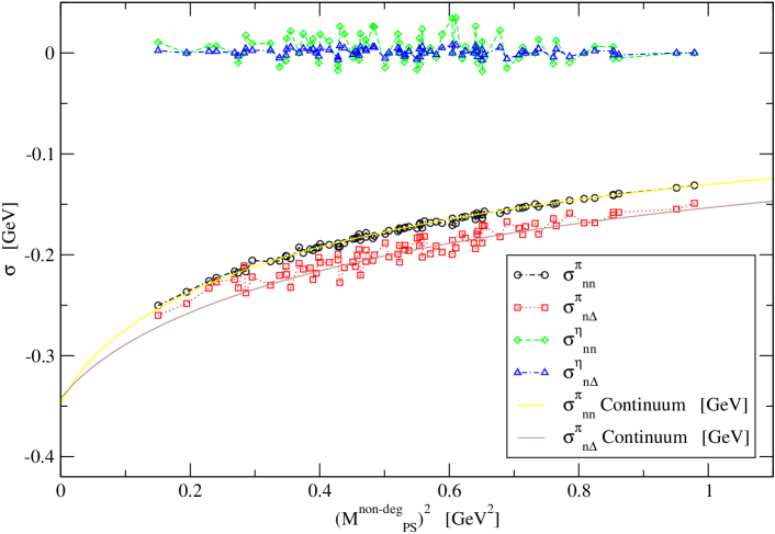
Figure 6.2: Here we plot the self-energy contributions (Eqs. 6.2) versus $(M_{PS}^{non-deg})^{2}$ for the entire degenerate data set (dashed lines are a guide for the eye only). We use the dipole form factor and choose an arbitrary value for the Lambda parameter, $\Lambda=1$ [GeV]. We also include continuum data (the straight lines) for the pion processes (the eta case vanishes in the physical limit) which is obtained by solving the self energy equations using a fourth order Runge-Kutta algorithm.

6.3 The CP-PACS Nucleon data

In this chapter we again use data published in [22]. Here we use the baryon data though. As before this data comes from dynamical simulations for mean-field improved Wilson fermions with improved gluons. We again study four different $\beta$ values which each have four different $\kappa_{\rm sea}$ values, giving 16 independent ensembles. The lattice parameters used have been summarised in table 5.1. Figure 5.4 is a graphical representation of the unitary pseudo-scalar masses plotted against the lattice spacing $a_{r_{0}}$ and we again recall that $(M_{PS}^{unit})^{2}$ is a direct measure of the sea quark mass (sec. 4.9.2). In this chapter we consider the same two methods of setting the scale as in chapter 5, namely from the string tension $(\sigma)$, and from the Sommer scale $(r_{0})$. The degenerate data set contains 80 data points (five $\kappa_{\rm val}$ values for each $(\beta,\kappa_{\rm sea})$ point), and as before we generate a 1000 bootstrap clusters for all $M_{PS}$ and $M_{N}$ data. The data has a Gaussian distribution with a central value equal the $M_{PS}$($M_{N}$) value published in table XXI(XXII - for the degenerate nucleon, XXIII - for the non-degenerate nucleon) of [22] and has a FWHM equal to the published error. As before (sec. 5.3) we use totally uncorrelated data throughout, hence we expect our statistical errors to be overestimates of the true error in our results. As before the lattice spacings $a_{\sigma}$ and $a_{r_{0}}$ are taken from table XII of [22]. We generate 1000 bootstrap clusters with the correct Gaussian and FWHM distribution. The values $r_{0}=0.49$ and $\sqrt{\sigma}=440$ MeV are used. Again we assume that the data has both ${\cal O}(a)$ and ${\cal O}(a^{2})$ lattice systematics which we investigate in section 6.4.

6.4 Fitting analysis

6.4.1 Summary of analysis techniques

The philosophy behind our fitting method remains the same as for our investigation of the meson spectrum (chap. 5), i.e. we work in physical units when performing our extrapolations. We do this because it allows us to combine data from different ensembles; this cannot be done for the dimensionless data because of differing lattice spacings. Also we expect that we will benefit from some cancellation of the systematic (and statistical) errors. This is because dimensionful mass predictions from lattice simulations are effectively mass ratios (sec. 5.4.1).

As mentioned previously we study two methods for setting the scale, using the string tension $(\sigma)$ and the Sommer scale $(r_{0})$. As with the meson analysis (chap. 5) we find a preferred method for setting the scale which we discuss in section 6.4.3.

We compare the Adelaide fitting procedure to the corresponding naive fitting function. After trying many different ways of fitting the data and allowing the error in the coefficients and the $\chi^{2}$ for these fits to guide us, we find that the data is best fitted by the following

$$M_{N}-\Sigma_{N} = a_{0}+a_{2}(M_{PS}^{deg})^{2}+a_{4}(M_{PS}^{deg})^{4}+a_{6}(M_{PS}^{deg})^{6}$$ (6.15)

The corresponding naive fitting function is

$$M_{N} = a_{0}+a_{2}(M_{PS}^{deg})^{2}+a_{4}(M_{PS}^{deg})^{4}+a_{6}(M_{PS}^{deg})^{6}$$ (6.16)

Again we divide these fits into two categories. These are referred to as “cubic” and “quadratic”. We remind the reader that this is because “cubic” fits include cubic terms in the chiral expansion of $m^{q}_{\rm sea}\propto(M_{PS}^{deg})^{2}$. The “quadratic” fits have the $a_{6}$ term set to zero and so have terms that are quadratic in $m^{q}_{\rm sea}$. We choose to use a subtracted fit for convenience. A fit that has the self-energy added to the RHS of equation 6.16 would be equally valid. In figure 6.3 we plot the dimensionful nucleon data and also the subtracted nucleon data. We see that the original data for the nucleon has some curvature but this is mostly corrected by subtracting the self-energy from it. So for high values of $\lambda$ we expect the higher order coefficients in the cubic fits to be poorly determined or approximately zero for the Adelaide case. Although this is the case, we will see that the data is better fitted by a moderate value of $\Lambda$.

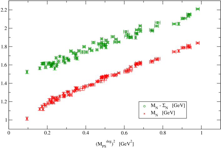
Figure 6.3: The nucleon mass and the subtracted nucleon mass versus $(M_{PS}^{deg})^{2}$ for the entire degenerate data set. Again we use the dipole form factor and we use the same arbitrary value for the Lambda parameter, $\Lambda=1$ [GeV]. The scale is set using the string tension $(\sigma)$.

In the next subsection we fit to equations 6.15 and 6.16 for the sixteen individual ensembles (table 5.1). Following this we fit to 6.15 and 6.16 for the entire degenerate data set (as in sec 5.4.3).

6.4.2 Individual ensemble fits

In this section we treat the sixteen ensembles separately. We do this by fitting to the five degenerate data points $(M^{deg}_{N},M^{deg}_{PS})$ in each $\beta,~{}\kappa_{\rm sea}$ ensemble. We use our preferred form factor which is the dipole form factor (sec 6.4.3 & sec 6.4.4) and we only consider the case where $r_{0}$ is used to set the scale. For the dipole form factor we choose a preferred value for $\Lambda$ (when setting the scale from $r_{0}$) of 600 [MeV]. Section 6.4.3 shows that the preferred value of $\Lambda$ has a slight dependency on the modelling of the lattice systematics, but this is a very small variation of approximately 1%. The fits considered in this section are quadratic, i.e. we set $a_{6}=0$. This is done because cubic fits for the individual case all have 100% error in the $a_{4}$ and $a_{6}$ coefficients. Table 6.1 lists the coefficients for both the Adelaide fits and also the naive fits.

	$\beta$	$\kappa_{sea}$	$a^{naive}_{0}$	$a^{adel}_{0}$	$a^{naive}_{2}$	$a^{adel}_{2}$	$a^{naive}_{4}$	$a^{adel}_{4}$
			[GeV]	[GeV]	[GeV-1]	[GeV-1]	[GeV-3]	[GeV-3]
	1.80	0.1409	0.97${\scriptstyle{}^{+{4}}_{-{4}}}$	1.03${\scriptstyle{}^{+{4}}_{-{4}}}$	1.11${\scriptstyle{}^{+{12}}_{-{14}}}$	1.09${\scriptstyle{}^{+{13}}_{-{14}}}$	-0.30${\scriptstyle{}^{+{15}}_{-{13}}}$	-0.29${\scriptstyle{}^{+{15}}_{-{14}}}$
	1.80	0.1430	0.98${\scriptstyle{}^{+{3}}_{-{2}}}$	1.04${\scriptstyle{}^{+{3}}_{-{2}}}$	1.11${\scriptstyle{}^{+{11}}_{-{12}}}$	1.08${\scriptstyle{}^{+{11}}_{-{12}}}$	-0.29${\scriptstyle{}^{+{13}}_{-{12}}}$	-0.29${\scriptstyle{}^{+{13}}_{-{13}}}$
	1.80	0.1445	0.96${\scriptstyle{}^{+{3}}_{-{3}}}$	1.03${\scriptstyle{}^{+{3}}_{-{3}}}$	1.21${\scriptstyle{}^{+{12}}_{-{11}}}$	1.18${\scriptstyle{}^{+{13}}_{-{12}}}$	-0.37${\scriptstyle{}^{+{13}}_{-{14}}}$	-0.37${\scriptstyle{}^{+{13}}_{-{14}}}$
	1.80	0.1464	0.93${\scriptstyle{}^{+{3}}_{-{3}}}$	1.01${\scriptstyle{}^{+{3}}_{-{3}}}$	1.27${\scriptstyle{}^{+{12}}_{-{10}}}$	1.23${\scriptstyle{}^{+{12}}_{-{11}}}$	-0.42${\scriptstyle{}^{+{12}}_{-{14}}}$	-0.41${\scriptstyle{}^{+{12}}_{-{14}}}$
	1.95	0.1375	1.00${\scriptstyle{}^{+{4}}_{-{3}}}$	1.05${\scriptstyle{}^{+{4}}_{-{3}}}$	1.08${\scriptstyle{}^{+{10}}_{-{12}}}$	1.07${\scriptstyle{}^{+{11}}_{-{12}}}$	-0.25${\scriptstyle{}^{+{10}}_{-{8}}}$	-0.25${\scriptstyle{}^{+{10}}_{-{9}}}$
	1.95	0.1390	1.00${\scriptstyle{}^{+{3}}_{-{2}}}$	1.06${\scriptstyle{}^{+{3}}_{-{2}}}$	1.04${\scriptstyle{}^{+{8}}_{-{8}}}$	1.02${\scriptstyle{}^{+{8}}_{-{8}}}$	-0.21${\scriptstyle{}^{+{7}}_{-{7}}}$	-0.20${\scriptstyle{}^{+{7}}_{-{7}}}$
	1.95	0.1400	0.99${\scriptstyle{}^{+{2}}_{-{2}}}$	1.05${\scriptstyle{}^{+{2}}_{-{2}}}$	1.11${\scriptstyle{}^{+{7}}_{-{7}}}$	1.08${\scriptstyle{}^{+{7}}_{-{7}}}$	-0.26${\scriptstyle{}^{+{6}}_{-{6}}}$	-0.25${\scriptstyle{}^{+{6}}_{-{6}}}$
	1.95	0.1410	1.01${\scriptstyle{}^{+{2}}_{-{2}}}$	1.07${\scriptstyle{}^{+{2}}_{-{2}}}$	1.08${\scriptstyle{}^{+{7}}_{-{6}}}$	1.05${\scriptstyle{}^{+{7}}_{-{6}}}$	-0.24${\scriptstyle{}^{+{6}}_{-{6}}}$	-0.23${\scriptstyle{}^{+{6}}_{-{7}}}$
	2.10	0.1357	1.04${\scriptstyle{}^{+{2}}_{-{2}}}$	1.08${\scriptstyle{}^{+{2}}_{-{2}}}$	1.06${\scriptstyle{}^{+{7}}_{-{7}}}$	1.05${\scriptstyle{}^{+{7}}_{-{7}}}$	-0.23${\scriptstyle{}^{+{5}}_{-{5}}}$	-0.23${\scriptstyle{}^{+{5}}_{-{5}}}$
	2.10	0.1367	1.05${\scriptstyle{}^{+{2}}_{-{2}}}$	1.10${\scriptstyle{}^{+{2}}_{-{2}}}$	1.01${\scriptstyle{}^{+{7}}_{-{7}}}$	0.99${\scriptstyle{}^{+{7}}_{-{7}}}$	-0.19${\scriptstyle{}^{+{5}}_{-{5}}}$	-0.19${\scriptstyle{}^{+{5}}_{-{5}}}$
	2.10	0.1374	1.04${\scriptstyle{}^{+{2}}_{-{2}}}$	1.10${\scriptstyle{}^{+{2}}_{-{2}}}$	1.03${\scriptstyle{}^{+{7}}_{-{7}}}$	1.01${\scriptstyle{}^{+{7}}_{-{7}}}$	-0.19${\scriptstyle{}^{+{5}}_{-{5}}}$	-0.19${\scriptstyle{}^{+{5}}_{-{5}}}$
	2.10	0.1382	1.00${\scriptstyle{}^{+{2}}_{-{2}}}$	1.06${\scriptstyle{}^{+{2}}_{-{2}}}$	1.13${\scriptstyle{}^{+{6}}_{-{6}}}$	1.10${\scriptstyle{}^{+{6}}_{-{6}}}$	-0.25${\scriptstyle{}^{+{4}}_{-{4}}}$	-0.25${\scriptstyle{}^{+{4}}_{-{4}}}$
	2.20	0.1351	1.04${\scriptstyle{}^{+{5}}_{-{5}}}$	1.08${\scriptstyle{}^{+{5}}_{-{5}}}$	1.0${\scriptstyle{}^{+{2}}_{-{2}}}$	1.0${\scriptstyle{}^{+{2}}_{-{2}}}$	-0.21${\scriptstyle{}^{+{12}}_{-{15}}}$	-0.21${\scriptstyle{}^{+{13}}_{-{15}}}$
	2.20	0.1358	1.10${\scriptstyle{}^{+{4}}_{-{4}}}$	1.14${\scriptstyle{}^{+{4}}_{-{4}}}$	0.87${\scriptstyle{}^{+{12}}_{-{13}}}$	0.86${\scriptstyle{}^{+{12}}_{-{14}}}$	-0.09${\scriptstyle{}^{+{10}}_{-{9}}}$	-0.08${\scriptstyle{}^{+{10}}_{-{9}}}$
	2.20	0.1363	1.04${\scriptstyle{}^{+{4}}_{-{4}}}$	1.08${\scriptstyle{}^{+{4}}_{-{4}}}$	1.03${\scriptstyle{}^{+{13}}_{-{11}}}$	1.01${\scriptstyle{}^{+{13}}_{-{12}}}$	-0.20${\scriptstyle{}^{+{8}}_{-{9}}}$	-0.19${\scriptstyle{}^{+{8}}_{-{9}}}$
	2.20	0.1368	1.01${\scriptstyle{}^{+{4}}_{-{3}}}$	1.06${\scriptstyle{}^{+{4}}_{-{3}}}$	1.08${\scriptstyle{}^{+{11}}_{-{11}}}$	1.05${\scriptstyle{}^{+{11}}_{-{11}}}$	-0.23${\scriptstyle{}^{+{8}}_{-{8}}}$	-0.22${\scriptstyle{}^{+{8}}_{-{8}}}$

Table 6.1: The coefficients obtained from fitting $M_{N}$ data against $M_{PS}^{2}$. We list results for both the naive and Adelaide fits (eqs. 6.16 & 6.15 respectively) for each of the 16 ensembles listed in Table 5.1. A dipole form factor was employed for the Adelaide fits using $\Lambda=600$ [MeV] and the scale was set from $r_{0}$.

As expected the leading Adelaide coefficient is always greater than the corresponding coefficient from the naive fits $(a^{adel}_{0}>a^{naive}_{0})$. In nearly all cases the $a_{2}$ coefficient is smaller for the Adelaide fits $(a^{adel}_{2}<a^{naive}_{2})$. The $a_{4}$ coefficients are approximately the same for both fits $(a^{adel}_{4}\sim a^{naive}_{4})$, but the error in this coefficient is very large, typically 50%. We see only a few cases where the $a_{4}$ coefficient is zero within errors though, indicating its presence is needed. Importantly nearly all of these coefficients are equal within errors.

There appears to be no overall trend with the sea quark mass for any of the coefficients. This indicates that unquenching effects are minimal.

Figure 6.4 is representative of all fits. It comes from the $(\beta,\kappa_{\rm sea})=(2.10,0.1382)$ ensemble. This data set is one of the closest to the physical point (fig 5.4).

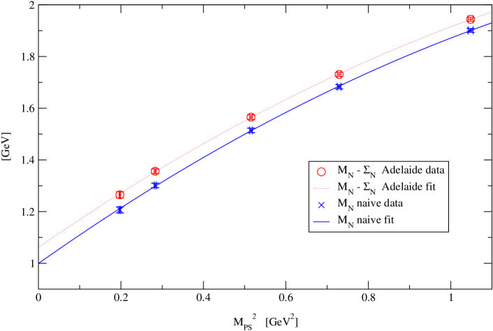
Figure 6.4: A plot of $M_{N}$ versus $M_{PS}^{2}$ for the ensemble $(\beta,\kappa_{\rm sea})=(2.10,0.1382)$. Included are the results of the quadratic naive (Eq. 6.16) and the quadratic Adelaide (Eq. 6.15) fits. The scale is set from $r_{0}$, we use a dipole form factor and our preferred value for $\Lambda$ ($\Lambda=600$ [MeV]).

We now go on to investigate the correlation between the coefficients $a_{0}$ and $a_{2}$. As can be observed in figures 6.5 and 6.6 there is a clear and well defined correlation between the $a_{0}$ and $a_{2}$ coefficients. As expected, when the value of $a_{0}$ increases, the value of $a_{2}$ decreases. The correlation here is far better than that observed in section 5.4.2 for the meson data.

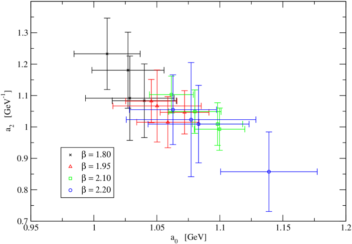
Figure 6.5: A scatter plot of $a_{2}$ against $a_{0}$ for the Adelaide fit investigating their mutual correlation.

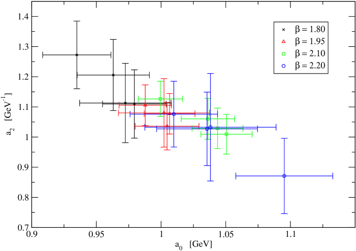
Figure 6.6: A scatter plot of $a_{2}$ against $a_{0}$ for the naive fit investigating their mutual correlation.

We now investigate the variation of the $a_{0,2}$ coefficients with the lattice spacing $a_{r_{0}}$. As in section 5.4.2 we plot $a_{0,2}$ against $a_{r_{0}}$ and use these plots (figs. 6.7 & 6.8) to motivate the following continuum extrapolation

$$a_{0,2}=a_{0,2}^{cont}+X^{individual}_{0,2}\;a_{r_{0}}$$ (6.17)

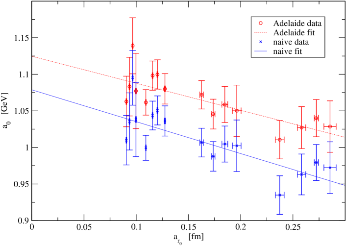
Figure 6.7: A continuum extrapolation of the $a_{0}$ coefficient obtained from both the Adelaide and naive fits Eq.(6.17).

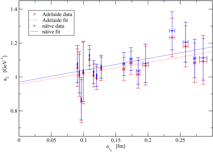
Figure 6.8: A continuum extrapolation of the $a_{2}$ coefficient obtained from both the Adelaide and naive fits Eq.(6.17).

Interestingly we investigated a continuum extrapolation of the form
$a_{0}=a_{0}^{cont}+X^{individual}_{0}\;a_{r_{0}}^{2}$ but found that the data was better fitted by equation 6.17. This is the case for both the Adelaide and naive data. It is at odds with section 6.4.3. The results of the fits corresponding to equation 6.17 are listed in table 6.2.

	$a_{0}^{cont.}$	$X^{individual}_{0}$	$\chi^{2}_{0}/d.o.f.$	$a_{2}^{cont.}$	$X^{individual}_{2}$	$\chi^{2}_{2}/d.o.f.$
	[GeV]	[GeV/fm]		[GeV-1]	[GeV-1/fm]
Naive-fit	1.08${\scriptstyle{}^{+{2}}_{-{2}}}$	-0.44${\scriptstyle{}^{+{10}}_{-{11}}}$	13 / 14	0.97${\scriptstyle{}^{+{7}}_{-{6}}}$	0.7${\scriptstyle{}^{+{4}}_{-{4}}}$	7 / 14
Adelaide-fit	1.12${\scriptstyle{}^{+{2}}_{-{2}}}$	-0.37${\scriptstyle{}^{+{10}}_{-{11}}}$	8 / 14	0.96${\scriptstyle{}^{+{7}}_{-{6}}}$	0.6${\scriptstyle{}^{+{4}}_{-{4}}}$	6 / 14

Table 6.2: The coefficients obtained from the continuum extrapolation of both the naive and Adelaide $a_{0,2}$ values from Table 6.1 using eq. 6.17.

We see that although errors are high for all values of $X^{individual}$ the better determined lattice spacing effect appears to be present in the leading coefficient $(a_{0})$. Because errors are so high in these coefficients we believe that this is a sign of there being minimal ${\cal O}(a)$ effects in the lattice data when the scale is set using $a_{r_{0}}$. We investigate this further in section 6.4.3.

To close this section we provide a brief investigation of the lattice nucleon data having a sea quark dependency. To do this we use the same method as in 5.4.2 i.e. we plot $a_{0,2}-X^{individual}_{0,2}a_{r_{0}}$ against $(M_{PS}^{unit})^{2}$. We remind the reader that we subtract $X^{individual}_{0,2}a_{r_{0}}$ in the $y-$coordinate in an attempt to leave the residual $m^{q}_{\rm sea}$ effects. The results of this can be seen in figures 6.9 & 6.10. We observe no discernible trend with the sea quark mass (from the PCAC relation, $(M_{PS}^{unit})^{2}\propto m^{q}_{\rm sea}$) for either of the coefficients. It can be seen however that as the mass of the pseudo-scalar decreases, the difference between the Adelaide and naive data points increases.

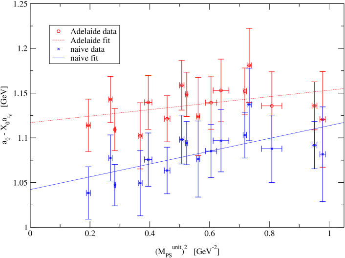
Figure 6.9: A chiral extrapolation of the $a_{0}-X^{individual}_{0}a$ coefficient obtained from both the linear and Adelaide fits. The scale was taken from $r_{0}$.

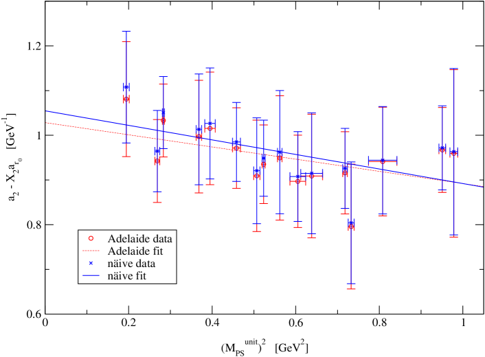
Figure 6.10: A chiral extrapolation of the $a_{2}-X^{individual}_{2}a$ coefficient obtained from both the linear and Adelaide fits. The scale was taken from $r_{0}$.

We conclude by noting that we have seen no strong evidence for unquenching effects in the data.

6.4.3 Global fits

We now analyse the complete degenerate data set by treating the 16 ensembles of section 6.4.2 in a global manner. This gives us 80 data points to work with. The larger data set should produce highly constrained fits (as seen in section 5.4.3). It is our hope that this larger data set will allow us to determine the higher order coefficients in our fitting functions (Eqs. 6.15 & 6.16). We give a graphical representation of the degenerate (80 data points) CP-PACS nucleon data in figures 6.11 and 6.12 where the scale has been set using the Sommer scale $(r_{0})$ and the string tension $(\sigma)$ respectively.

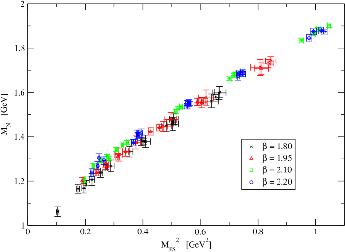
Figure 6.11: A plot of the degenerate CP-PACS nucleon data set. Here the scale is set using $r_{0}$.

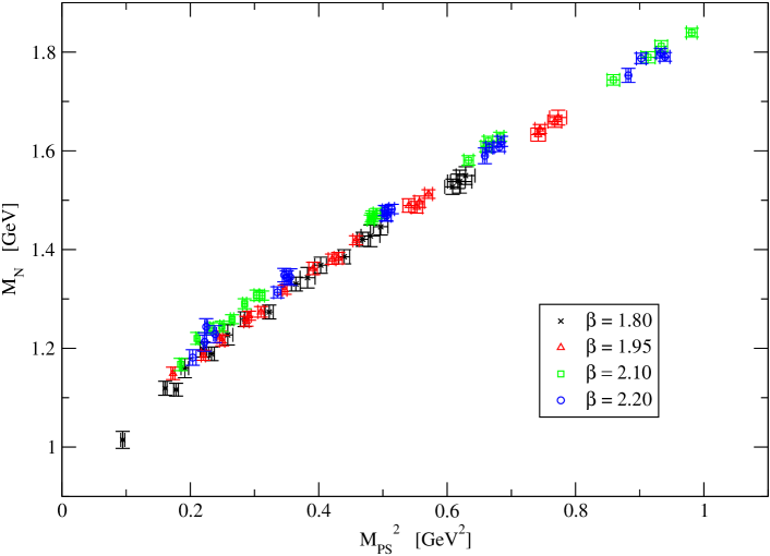
Figure 6.12: A plot of the degenerate CP-PACS nucleon data set. Here the scale is set using $\sigma$.

As can be seen the data in these plots has clear curvature, moreover the agreement between data from different $(\beta,\kappa_{\rm sea})$ values is quite remarkable when we consider that these plots are representative of the degenerate data set and have had nothing done to them to correct for lattice artefacts. When treating the data in a global manner it is very important to ensure that the lattice spacing artefacts are modelled correctly. To this end we use the investigations of the previous section and all we have learnt from the mesonic data (chap. 5) to guide us when trying to account for lattice spacing effects. We have studied many different fitting functions where we try fitting forms that include ${\cal O}(a,a^{2})$ terms in the $a_{2}$ and higher coefficients. We have found though that these fits are unstable. Hence we conclude that for the global method lattice spacing artifacts are dominant in the leading coefficient $(a_{0})$. Hence we believe that accounting for ${\cal O}(a)$ and ${\cal O}(a^{2})$ errors in the $a_{0}$ coefficient will be enough to correct for any significant lattice spacing effects present in the data. We choose ${\cal O}(a)$ and ${\cal O}(a^{2})$ corrections because the lattice action is tree-level improved and so should contain ${\cal O}(a^{2})$ errors together with a small amount of ${\cal O}(a)$ errors but as seen in chapter 5, when the scale is set using the string tension, ${\cal O}(a)$ errors seem to dominate. Therefore our preferred fits, which are modified versions of equations 6.15 and 6.16, are

$$M_{N}-\Sigma_{N} = (a_{0}+X_{n}a^{n})+a_{2}(M_{PS}^{deg})^{2}+a_{4}(M_{PS}^{deg})^{4}+a_{6}(M_{PS}^{deg})^{6}$$ (6.18)

and the corresponding naive fitting function for the global case is

$$M_{N} = (a_{0}+X_{n}a^{n})+a_{2}(M_{PS}^{deg})^{2}+a_{4}(M_{PS}^{deg})^{4}+a_{6}(M_{PS}^{deg})^{6}$$ (6.19)

As discussed in the summery of our fitting analysis (sec 6.4.1) we divide these fits into two categories. These are referred to as “cubic” and “quadratic”. As before this is because “cubic” fits include cubic terms in the chiral expansion of $m^{q}_{\rm sea}\propto(M_{PS}^{deg})^{2}$. The “quadratic” fits have the $a_{6}$ term set to zero and so have terms that are at most quadratic in $m^{q}_{\rm sea}$. These two categories are divided into two further sub-categories. The first sub-category contains the fitting functions that have corrections for ${\cal O}(a)$ lattice spacing effects in the $a_{0}$ coefficient, i.e. we have $n=1$ in equations 6.18 and 6.19. The second sub-category contains the fitting functions that have ${\cal O}(a^{2})$ corrections for lattice spacing effects in the $a_{0}$ coefficient, i.e. we have $n=2$ in equations 6.18 and 6.19. Hence for the global fit analysis the maximum number of fit parameters in any one fitting function is five. Our data set contains 80 points so we hope that this method will provide highly constrained fit parameters compared to those from the individual fitting method (sec 6.4.2). This is because for the individual fitting method the number of fit parameters was three, but the number of data points in each $(\beta,\kappa_{\rm sea})$ ensemble was only five.

In this subsection we study two different methods for setting the scale. We remind the reader the previous section only studied one method of setting the scale. Here we set the scale using the Sommer scale $(r_{0})$, and from the string tension, $(\sigma)$. Finally for the Adelaide method we have two different form factors to study (as outlined in sections 6.1 & 6.2). These are the dipole and Gaussian form factors given by equations 6.9 and 6.10 respectively. Hence for the naive fitting method we have $2^{3}$ different fitting procedures, and for the Adelaide method we have $2^{4}$ different fitting methods. These fitting methods are summarised in table 6.3. As in section 5.4.3, any one of these fits can be built by moving from left to right in table 6.3 and making a choice in each column.

Approach	Form Factor	Chiral Extrapolation	Treatment of Lattice	Lattice Spacing
			Spacing Artifacts in $a_{0}$	set from
Adelaide	dipole	Cubic	$a_{0}$ term has	$r_{0}$
i.e. eq.5.14	Gaussian	i.e. ${\cal O}(M_{PS}^{6})$ included	${\cal O}(a)$ corrections
Naive	-	Quadratic	$a_{0}$ term has	$\sigma$
i.e. eq.5.15		i.e. no ${\cal O}(M_{PS}^{6})$ term	${\cal O}(a^{2})$ corrections

Table 6.3: The different fit types used in the global analysis.

As demonstrated in section 5.4.3 of chapter 5, when performing the Adelaide fits we have to determine a best value for the $\Lambda$ parameter. We remind the reader that $\Lambda$ is a length scale and it is this parameter that models the size of the quasi-particle that we are studying. Hence it is this that controls the chiral physics. Again because we use a subtracted style of fit it is not possible to allow $\Lambda$ to be a free parameter in the fit. We have, in our early works, studied fitting functions that allow $\Lambda$ to be a free parameter in the fit but found that these fits were highly unstable. Instead we use the method outlined in section 5.4.3. This is where we manually vary the lambda parameter then plot the $\chi^{2}/d.o.f$ for each different fitting function against $\Lambda$. Figures 6.13 and 6.14 represent this for the dipole and Gaussian form factors respectively.

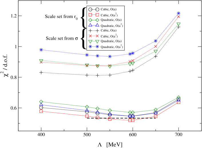
Figure 6.13: A plot of $\chi^{2}/d.o.f$ against $\Lambda$ for the dipole form factor. The dashed horizontal line represents increasing $\chi^{2}$ from its minimum value by unity for the $r_{0}$ data (i.e. it represents one standard deviation). The intercept of this dashed line with the $\chi^{2}$ curves (at $\Lambda=$535 and 626 MeV) is used to derive upper and lower bounds for the preferred $\Lambda$ value for the dipole case.

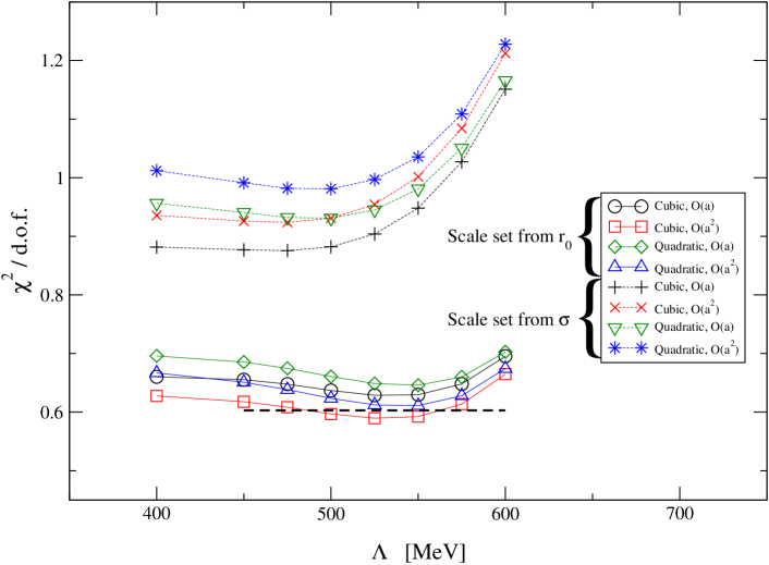
Figure 6.14: A plot of $\chi^{2}/d.o.f$ against $\Lambda$ for the Gaussian form factor. The dashed horizontal line represents increasing $\chi^{2}$ from its minimum value by unity for the $r_{0}$ data (i.e. it represents one standard deviation). The intercept of this dashed line with the $\chi^{2}$ curves (at $\Lambda=$486 and 562 MeV) is used to derive upper and lower bounds for the preferred $\Lambda$ value for the Gaussian case.

When the scale is set from $r_{0}$ we see that the $\chi^{2}/d.o.f$ as a function of $\Lambda$ has a similar functional form for all fitting functions. The plots also show that the preferred value of $\Lambda$ has a small dependency on the order of the chiral expansion. For the dipole case this is very small of the order of 1% and for the Gaussian case it is nearer 5%. Note though the change in $\chi^{2}/d.o.f$ as $\Lambda$ is varied is less for the Gaussian case. We observe no dependence of the preferred value of $\Lambda$ on the modelling of the lattice systematics. We also see that the better $\chi^{2}/d.o.f$ is given when the dipole form factor is used. As expected we see that the preferred value of $\Lambda$ is dependent on the type of form factor used. When setting the scale from $r_{0}$ our preferred values of $\Lambda$ are

Quadratic $$\Biggl{\{} \begin{array}[]{lcl}\Lambda^{dipole}_{r_{0}}&=&600\\ \Lambda^{Gaussian}_{r_{0}}&=&550\end{array}\hskip 28.45274pt\textrm{[MeV]}$$ (6.22)

Cubic $$\Biggl{\{} \begin{array}[]{lcl}\Lambda^{dipole}_{r_{0}}&=&594_{-59}^{+32}\\ \Lambda^{Gaussian}_{r_{0}}&=&525_{-39}^{+37}\end{array}\hskip 14.22636pt\textrm{[MeV]}$$ (6.25)

When the scale is set from $\sigma$ the plots again show a similar functional form for the $\chi^{2}/d.o.f$ for all fitting functions. We see that the preferred value of $\Lambda$ again has a dependence on the order of the chiral expansion which is about 5%. As in the case where the scale is set from $r_{0}$ the preferred value of $\Lambda$ has no dependence on the modelling of the lattice artifacts. When setting the scale from $\sigma$ our preferred values of $\Lambda$ are

Quadratic $$\Biggl{\{} \begin{array}[]{lcl}\Lambda^{dipole}_{\sigma}&=&550\\ \Lambda^{Gaussian}_{\sigma}&=&500\end{array}\hskip 28.45274pt\textrm{[MeV]}$$ (6.28)

Cubic $$\Biggl{\{} \begin{array}[]{lcl}\Lambda^{dipole}_{\sigma}&=&523\\ \Lambda^{Gaussian}_{\sigma}&=&475\end{array}\hskip 28.45274pt\textrm{[MeV]}$$ (6.31)

Figures 6.13 and 6.14 show that as expected the preferred value of $\Lambda$ is dependent on the form factor used, but it is also dependent on the method used to set the scale. This discrepancy was discussed in section 5.5.1 of chapter 5 in terms of the mesonic data. We will address the case for the nucleons in section 6.6.

We see that (as with the mesonic data in chapter 5), when the scale is set from $r_{0}$, ${\cal O}(a^{2})$ errors dominate. But when the scale is set from $\sigma$, ${\cal O}(a)$ errors dominate. This is further evidence supporting the idea that in cases where the scale is set using $\sigma$ the dominant lattice spacing systematics will be ${\cal O}(a)$ and in cases where the scale is set from $r_{0}$ the dominant lattice spacing systematics will be ${\cal O}(a^{2})$. As in chapter 5 we have no explanation as to why this should be the case.

We use these preferred values of $\Lambda$ to perform the 16 Adelaide fits outlined in table 6.3 and the 8 naive fits that are also listed in table 6.3. The results of these fits along with the $\chi^{2}/d.o.f$ for each fit are listed in tables 6.4 and 6.5 for the cases where the scale is set from $r_{0}$ and $\sigma$ respectively.

Fit	Form	$a_{0}^{cont}$	$X_{0}$	$X_{2}$	$a_{2}$	$a_{4}$	$a_{6}$	$\chi^{2}/d.o.f.$
Approach	Factor	[GeV]	[GeVfm-1]	[GeVfm-2]	[GeV-1]	[GeV-3]	[GeV-5]
Cubic chiral extrapolation        $a_{0}$ contains ${\cal O}(a)$
Adelaide	dipole	1.08${\scriptstyle{}^{+{2}}_{-{2}}}$	-0.23${\scriptstyle{}^{+{2}}_{-{3}}}$	-	1.20${\scriptstyle{}^{+{9}}_{-{9}}}$	-0.5${\scriptstyle{}^{+{2}}_{-{2}}}$	0.17${\scriptstyle{}^{+{9}}_{-{9}}}$	41 / 75
Adelaide	Gaussian	1.08${\scriptstyle{}^{+{2}}_{-{2}}}$	-0.22${\scriptstyle{}^{+{2}}_{-{3}}}$	-	1.19${\scriptstyle{}^{+{10}}_{-{9}}}$	-0.5${\scriptstyle{}^{+{2}}_{-{2}}}$	0.16${\scriptstyle{}^{+{9}}_{-{9}}}$	47 / 75
Naive	-	1.02${\scriptstyle{}^{+{2}}_{-{2}}}$	-0.27${\scriptstyle{}^{+{2}}_{-{3}}}$	-	1.29${\scriptstyle{}^{+{10}}_{-{9}}}$	-0.6${\scriptstyle{}^{+{2}}_{-{2}}}$	0.21${\scriptstyle{}^{+{9}}_{-{9}}}$	45 / 75
Cubic chiral extrapolation        $a_{0}$ contains ${\cal O}(a^{2})$
Adelaide	dipole	1.060${\scriptstyle{}^{+{14}}_{-{16}}}$	-	-0.62${\scriptstyle{}^{+{6}}_{-{8}}}$	1.21${\scriptstyle{}^{+{10}}_{-{8}}}$	-0.53${\scriptstyle{}^{+{15}}_{-{18}}}$	0.17${\scriptstyle{}^{+{9}}_{-{8}}}$	39 / 75
Adelaide	Gaussian	1.059${\scriptstyle{}^{+{14}}_{-{16}}}$	-	-0.60${\scriptstyle{}^{+{6}}_{-{8}}}$	1.19${\scriptstyle{}^{+{10}}_{-{8}}}$	-0.51${\scriptstyle{}^{+{15}}_{-{18}}}$	0.16${\scriptstyle{}^{+{9}}_{-{8}}}$	44 / 75
Naive	-	0.999${\scriptstyle{}^{+{13}}_{-{17}}}$	-	-0.74${\scriptstyle{}^{+{6}}_{-{8}}}$	1.30${\scriptstyle{}^{+{10}}_{-{8}}}$	-0.64${\scriptstyle{}^{+{15}}_{-{18}}}$	0.22${\scriptstyle{}^{+{9}}_{-{8}}}$	44 / 75
Quadratic chiral extrapolation        $a_{0}$ contains ${\cal O}(a)$
Adelaide	dipole	1.106${\scriptstyle{}^{+{7}}_{-{8}}}$	-0.23${\scriptstyle{}^{+{2}}_{-{3}}}$	-	1.03${\scriptstyle{}^{+{2}}_{-{2}}}$	-0.210${\scriptstyle{}^{+{15}}_{-{17}}}$	-	43 / 76
Adelaide	Gaussian	1.101${\scriptstyle{}^{+{7}}_{-{8}}}$	-0.22${\scriptstyle{}^{+{2}}_{-{3}}}$	-	1.03${\scriptstyle{}^{+{2}}_{-{2}}}$	-0.207${\scriptstyle{}^{+{15}}_{-{17}}}$	-	49 / 76
Naive	-	1.056${\scriptstyle{}^{+{7}}_{-{8}}}$	-0.28${\scriptstyle{}^{+{2}}_{-{3}}}$	-	1.07${\scriptstyle{}^{+{2}}_{-{2}}}$	-0.230${\scriptstyle{}^{+{15}}_{-{17}}}$	-	49 / 76
Quadratic chiral extrapolation        $a_{0}$ contains ${\cal O}(a^{2})$
Adelaide	dipole	1.088${\scriptstyle{}^{+{6}}_{-{7}}}$	-	-0.63${\scriptstyle{}^{+{6}}_{-{8}}}$	1.03${\scriptstyle{}^{+{2}}_{-{2}}}$	-0.209${\scriptstyle{}^{+{15}}_{-{17}}}$	-	42 / 76
Adelaide	Gaussian	1.084${\scriptstyle{}^{+{6}}_{-{7}}}$	-	-0.61${\scriptstyle{}^{+{6}}_{-{8}}}$	1.03${\scriptstyle{}^{+{2}}_{-{2}}}$	-0.206${\scriptstyle{}^{+{15}}_{-{17}}}$	-	47 / 76
Naive	-	1.034${\scriptstyle{}^{+{6}}_{-{7}}}$	-	-0.75${\scriptstyle{}^{+{6}}_{-{8}}}$	1.07${\scriptstyle{}^{+{2}}_{-{2}}}$	-0.230${\scriptstyle{}^{+{15}}_{-{17}}}$	-	48 / 76

Table 6.4: The results of the global fit analysis where the scale is set from $r_{0}$.

Fit	Form	$a_{0}^{cont}$	$X_{0}$	$X_{2}$	$a_{2}$	$a_{4}$	$a_{6}$	$\chi^{2}/d.o.f.$
Approach	Factor	[GeV]	[GeVfm-1]	[GeVfm-2]	[GeV-1]	[GeV-3]	[GeV-5]
Cubic chiral extrapolation        $a_{0}$ contains ${\cal O}(a)$
Adelaide	dipole	1.001${\scriptstyle{}^{+{15}}_{-{14}}}$	-0.18${\scriptstyle{}^{+{2}}_{-{2}}}$	-	1.32${\scriptstyle{}^{+{9}}_{-{9}}}$	-0.7${\scriptstyle{}^{+{2}}_{-{2}}}$	0.28${\scriptstyle{}^{+{10}}_{-{10}}}$	61 / 75
Adelaide	Gaussian	1.002${\scriptstyle{}^{+{14}}_{-{14}}}$	-0.17${\scriptstyle{}^{+{2}}_{-{2}}}$	-	1.30${\scriptstyle{}^{+{9}}_{-{8}}}$	-0.7${\scriptstyle{}^{+{2}}_{-{2}}}$	0.27${\scriptstyle{}^{+{10}}_{-{10}}}$	66 / 75
Naive	-	0.966${\scriptstyle{}^{+{15}}_{-{14}}}$	-0.21${\scriptstyle{}^{+{2}}_{-{2}}}$	-	1.39${\scriptstyle{}^{+{9}}_{-{9}}}$	-0.8${\scriptstyle{}^{+{2}}_{-{2}}}$	0.33${\scriptstyle{}^{+{10}}_{-{10}}}$	62 / 75
Cubic chiral extrapolation        $a_{0}$ contains ${\cal O}(a^{2})$
Adelaide	dipole	0.986${\scriptstyle{}^{+{12}}_{-{14}}}$	-	-0.48${\scriptstyle{}^{+{6}}_{-{6}}}$	1.32${\scriptstyle{}^{+{9}}_{-{8}}}$	-0.7${\scriptstyle{}^{+{2}}_{-{2}}}$	0.29${\scriptstyle{}^{+{10}}_{-{9}}}$	66 / 75
Adelaide	Gaussian	0.988${\scriptstyle{}^{+{12}}_{-{14}}}$	-	-0.44${\scriptstyle{}^{+{6}}_{-{6}}}$	1.30${\scriptstyle{}^{+{9}}_{-{8}}}$	-0.7${\scriptstyle{}^{+{2}}_{-{2}}}$	0.28${\scriptstyle{}^{+{10}}_{-{9}}}$	69 / 75
Naive	-	0.947${\scriptstyle{}^{+{13}}_{-{14}}}$	-	-0.56${\scriptstyle{}^{+{6}}_{-{6}}}$	1.39${\scriptstyle{}^{+{9}}_{-{8}}}$	-0.8${\scriptstyle{}^{+{2}}_{-{2}}}$	0.33${\scriptstyle{}^{+{10}}_{-{9}}}$	68 / 75
Quadratic chiral extrapolation        $a_{0}$ contains ${\cal O}(a)$
Adelaide	dipole	1.036${\scriptstyle{}^{+{7}}_{-{7}}}$	-0.19${\scriptstyle{}^{+{2}}_{-{2}}}$	-	1.08${\scriptstyle{}^{+{2}}_{-{2}}}$	-0.24${\scriptstyle{}^{+{2}}_{-{2}}}$	-	67 / 76
Adelaide	Gaussian	1.036${\scriptstyle{}^{+{7}}_{-{7}}}$	-0.17${\scriptstyle{}^{+{2}}_{-{2}}}$	-	1.08${\scriptstyle{}^{+{2}}_{-{2}}}$	-0.23${\scriptstyle{}^{+{2}}_{-{2}}}$	-	71 / 76
Naive	-	1.006${\scriptstyle{}^{+{6}}_{-{7}}}$	-0.22${\scriptstyle{}^{+{2}}_{-{2}}}$	-	1.11${\scriptstyle{}^{+{2}}_{-{2}}}$	-0.26${\scriptstyle{}^{+{2}}_{-{2}}}$	-	69 / 76
Quadratic chiral extrapolation        $a_{0}$ contains ${\cal O}(a^{2})$
Adelaide	dipole	1.020${\scriptstyle{}^{+{6}}_{-{6}}}$	-	-0.49${\scriptstyle{}^{+{6}}_{-{6}}}$	1.08${\scriptstyle{}^{+{2}}_{-{2}}}$	-0.23${\scriptstyle{}^{+{2}}_{-{2}}}$	-	71 / 76
Adelaide	Gaussian	1.021${\scriptstyle{}^{+{6}}_{-{6}}}$	-	-0.46${\scriptstyle{}^{+{6}}_{-{6}}}$	1.07${\scriptstyle{}^{+{2}}_{-{2}}}$	-0.23${\scriptstyle{}^{+{2}}_{-{2}}}$	-	75 / 76
Naive	-	0.987${\scriptstyle{}^{+{6}}_{-{6}}}$	-	-0.58${\scriptstyle{}^{+{6}}_{-{6}}}$	1.11${\scriptstyle{}^{+{2}}_{-{2}}}$	-0.25${\scriptstyle{}^{+{2}}_{-{2}}}$	-	75 / 76

Table 6.5: The results of the global fit analysis where the scale is set from $\sigma$.

As with our global study of the mesonic data (sec 5.4.3) we conclude this section by summarising the results of the global fitting analysis (tables 6.4 & 6.5 and figs 6.13 & 6.14).

• Fit approach
  We see that the best $\chi^{2}/d.o.f.$ (indicating the best fitting procedure) is given by the Adelaide method which uses a dipole form factor. This has the best $\chi^{2}/d.o.f.$ in every case. This is further supporting evidence for the Adelaide method being a valid chiral extrapolation procedure. This is true for both methods of setting the scale. When a Gaussian form factor is employed we see that the $\chi^{2}/d.o.f.$ for the Adelaide method is roughly equal to that of the naive fit when the scale is set from $r_{0}$. When the scale is set from $\sigma$ we see that the naive method performs slightly better than the Adelaide method when a Gaussian form factor is used. We believe that this indicates that the Gaussian form factor does not represent the continuum behaviour of the pions in the quasi-particle correctly.

• Chiral extrapolation
  Errors in the higher order coefficients are large for the cubic fits compared to their quadratic counterparts. This said, the cubic fits always produce a non-zero $a_{6}$ coefficient indicating the need for a cubic term in $m^{q}_{sea}$. (Note that the quadratic fits were preferred in the mesonic case.)

• Treatment of the lattice spacing systematics and the fit coefficients
  We note the remarkable agreement between the coefficients of the Adelaide dipole and Adelaide Gaussian fits for each fitting procedure. Moreover the coefficients of the Adelaide fits agree for the same order of the chiral expansion (cubic and quadratic fits). We see that the $X_{n}$ coefficients differ between the various fitting methods. We believe this is an indication that the lattice spacing error contained in the $a_{0}$ coefficient is more complicated that a simple ${\cal O}(a)$ or ${\cal O}(a^{2})$ error. Though we still believe that ${\cal O}(a)$ errors dominate when the scale is set from $\sigma$ and ${\cal O}(a^{2})$ errors are dominant when the scale is set from $r_{0}$.

• Setting the scale
  As seen in our study of the mesonic data (sec 5.4.3), the $\chi^{2}/d.o.f.$ is almost halved when the scale is set from $r_{0}$ compared to when the scale is set from $\sigma$ (figs 6.13 & 6.14). This, along with strong evidence for ${\cal O}(a)$ lattice systematics in the $\sigma$ data, gives us reason to favour setting the scale from $r_{0}$. We also note that in this study the naive method seems to prefer setting the scale from $r_{0}$, whereas in our study of the mesonic data (sec 5.4.3) the naive method seemed to have no preference.

Using our results from this section we select the cubic chiral extrapolation method with an ${\cal O}(a^{2})$ correction in the $a_{0}$ coefficient with the scale set from $r_{0}$ to define the central values of the Adelaide and naive methods. We favour a dipole form factor for the Adelaide method. The spread from the other fitting types is used to define the error. Section 6.5 contains physical predictions from the nucleon mass.

6.4.4 Analysis of the different form factors

In this subsection we include a brief study of the two form factors that are employed in this chapter (dipole eq 6.9 & Gaussian eq 6.10). We do this in an attempt to prove that the Adelaide method can employ different functional forms for the form factor $u(k)$ and still produce similar results (within errors). We note though that the results from the previous subsection (sec 6.4.3) indicate a preference for the dipole form factor. Figure 6.15 shows a 2D plot of the two form factors with $\Lambda$ set equal to the preferred values for each form factor (eqs 6.22 & 6.28).

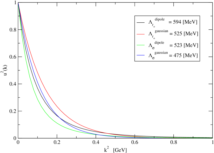
Figure 6.15: A plot of the dipole and Gaussian form factors. Calculated at the preferred values of $\Lambda$ for each form factor.

The plot shows for the preferred values of $\Lambda$ the functional forms of the dipole and Gaussian form factors are similar. It is clear though the dipole provides a sharper cut-off compared to the Gaussian. For a more intuitive view of how the form factors behave we include 3D plots for the dipole and Gaussian form factors (figs 6.16 & 6.17) showing how their functional form behaves as $\Lambda$ and $k^{2}$ change.

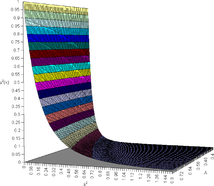
Figure 6.16: A 3D plot of the dipole form factor. The plot shows how the form factor behaves as $\Lambda$ and $k^{2}$ change.

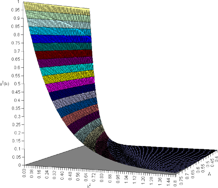
Figure 6.17: A 3D plot of the Gaussian form factor. The plot shows how the form factor behaves as $\Lambda$ and $k^{2}$ change.

We see that while the two plots show similar behaviour for smaller values of $\Lambda$, their behaviour changes as $\Lambda$ increases. For large values of $\Lambda$ the dipole provides a far sharper cut-off compared to the Gaussian form factor. It would be reasonable to assume that this is why the preferred values of $\Lambda$ are smaller in the Gaussian case compared to the dipole case. This provides evidence for the data selecting a form factor which has a functional form that most closely represents the continuum behaviour of the chiral physics. Since the data cannot alter the function which is used as the form factor it changes the $\Lambda$ parameter to suit. We offer further evidence for this in the form of figures 6.18 and 6.19. Here we see the behaviour of the self energy when the scale is set from $r_{0}$. Figure 6.18 represents the self energy data for a dipole form factor with the $\Lambda$ parameter set to our preferred value for this case which is 594 [MeV]. Figure 6.19 represents the self energy data for a Gaussian form factor with the $\Lambda$ parameter set to our preferred value for this case which is 525 [MeV].

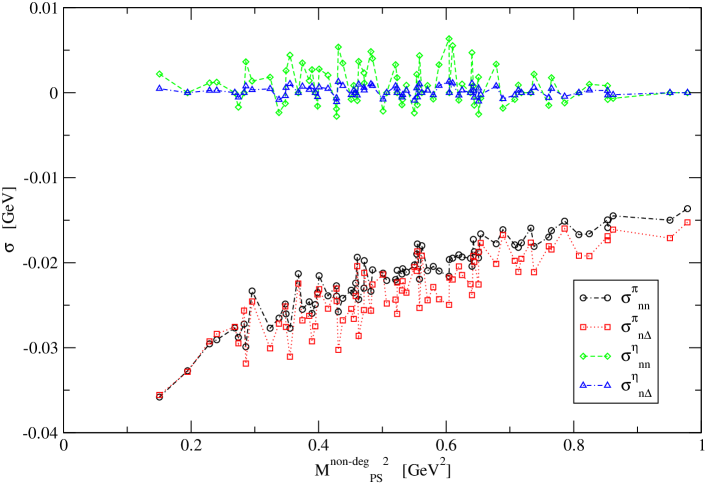
Figure 6.18: This plot shows how the self energy behaves when a dipole form factor is used and the scale is set from $r_{0}$. We use our preferred value of $\Lambda$ in this case which is 594 [MeV].

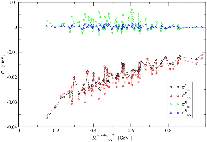
Figure 6.19: This plot shows how the self energy behaves when a Gaussian form factor is used and the scale is set from $r_{0}$. We use our preferred value of $\Lambda$ in this case which is 525 [MeV].

Although different form factors have been used, the resulting functional form of the self energy appears to be very similar. Importantly the energy scale that the self energy covers is almost identical. We see that the data for the dipole case has a smaller spread and this may contribute to the reduction in the $\chi^{2}/d.o.f$ in our fits.

We conclude this section by noting that the Adelaide method seems to prefer a value for the $\Lambda$ parameter that causes the form factor to represent the chiral physics in the continuum.

6.5 Physical predictions

In this section we make a physical prediction for the continuum nucleon mass $(M_{N})$. This is done for the Adelaide method (for both types of form factor) and also for the naive method (eqs 6.18 & 6.19). All of our predictions in this section will come from our global approach (studied in section 6.4.3) rather than the individual approach that was employed in section 6.4.2. We choose to use the global method because we expect the coefficients from this method to be more accurate than those from the individual approach since these fits should be highly constrained. Here we also include a study of the nucleon mass prediction $(M_{N})$ as a function of $\Lambda$. We obtain our continuum predictions by setting $M_{PS}^{deg}=M_{PS}^{non-deg}=M_{PS}^{unit}=\mu_{\pi}$ in equations 6.18, 6.19 and 6.2 with $\mu_{\pi}$ being the physical pion mass which we take to be $138$ [MeV]. We also set $M_{N}^{deg}=M_{N}^{non-deg}$ and $M_{\Delta}^{deg}=M_{\Delta}^{non-deg}$ in equation 6.2. In doing this we see that the $\eta^{\prime}$ contributions to the total self energy (eqs 6.11 & 6.2) disappear in the continuum as required. The only remaining term involving $M_{N}$ and $M_{\Delta}$ is the $\sigma^{\pi}_{N\Delta}$ self energy term. We set this equal to the physical mass splitting of the nucleon and $\Delta$ which we take to be $293$ [MeV] [33]. To calculate the self-energy terms in the continuum we use the same fourth order Runge-Kutta method that we employed in chapter 5. To make a physical prediction for each different fitting method (table 6.3) we use the coefficients $(a_{0}^{cont},~{}a_{2},~{}a_{4}~{}\&~{}a_{6})$ listed in tables 6.4 and 6.5 for the cases where $r_{0}$ and $\sigma$ are used to set the scale respectively. We list the results for our physical predictions in table 6.6. We use the relevant preferred value of $\Lambda$ for each Adelaide fit (taken from equations 6.22 & 6.28 for the scale set from $r_{0}$ and $\sigma$ respectively).

Estimate	Form	$M_{N}$ [GeV]	$M_{N}$ [GeV]
Approach	Factor	(Scale from $r_{0}$)	(Scale from $\sigma$)
Experimental	-	0.939	0.939
Cubic chiral extrapolation        $a_{0}$ contains ${\cal O}(a)$
Adelaide	dipole	0.984${\scriptstyle{}^{+{15}}_{-{15}}}$	0.950${\scriptstyle{}^{+{13}}_{-{13}}}$
Adelaide	Gaussian	0.973${\scriptstyle{}^{+{15}}_{-{15}}}$	0.938${\scriptstyle{}^{+{12}}_{-{13}}}$
Naive	-	1.046${\scriptstyle{}^{+{15}}_{-{15}}}$	0.992${\scriptstyle{}^{+{13}}_{-{13}}}$
Cubic chiral extrapolation        $a_{0}$ contains ${\cal O}(a^{2})$
Adelaide	dipole	0.965${\scriptstyle{}^{+{12}}_{-{15}}}$	0.934${\scriptstyle{}^{+{11}}_{-{12}}}$
Adelaide	Gaussian	0.956${\scriptstyle{}^{+{12}}_{-{15}}}$	0.923${\scriptstyle{}^{+{11}}_{-{12}}}$
Naive	-	1.023${\scriptstyle{}^{+{12}}_{-{15}}}$	0.974${\scriptstyle{}^{+{11}}_{-{12}}}$
Quadratic chiral extrapolation        $a_{0}$ contains ${\cal O}(a)$
Adelaide	dipole	1.006${\scriptstyle{}^{+{7}}_{-{8}}}$	0.974${\scriptstyle{}^{+{6}}_{-{6}}}$
Adelaide	Gaussian	0.986${\scriptstyle{}^{+{7}}_{-{8}}}$	0.959${\scriptstyle{}^{+{6}}_{-{6}}}$
Naive	-	1.076${\scriptstyle{}^{+{7}}_{-{8}}}$	1.027${\scriptstyle{}^{+{6}}_{-{6}}}$
Quadratic chiral extrapolation        $a_{0}$ contains ${\cal O}(a^{2})$
Adelaide	dipole	0.988${\scriptstyle{}^{+{6}}_{-{7}}}$	0.958${\scriptstyle{}^{+{5}}_{-{6}}}$
Adelaide	Gaussian	0.969${\scriptstyle{}^{+{6}}_{-{7}}}$	0.945${\scriptstyle{}^{+{5}}_{-{6}}}$
Naive	-	1.054${\scriptstyle{}^{+{6}}_{-{7}}}$	1.008${\scriptstyle{}^{+{5}}_{-{6}}}$

Table 6.6: Estimates of $M_{N}$ obtained from the global fits. Our experimental estimate comes from a simple average of the proton and neutron masses.

In figures 6.20 and 6.21 we present a graphical representation of our study into the variation of $M_{N}$ with the $\Lambda$ parameter for the dipole and Gaussian form factors respectively. Each figure contains eight data sets corresponding to the four different types of Adelaide fit and the two ways to set the scale. For each of these plots we include an acceptable range for the $\Lambda$ parameter which is represented by two vertical dashed lines. To find this range we use our plots of $\chi^{2}/d.o.f$ against $\Lambda$ (figs 6.13 & 6.14). We define the range of acceptable values of $\Lambda$ by increasing $\chi^{2}$ from its minimum by unity. This represents one standard deviation. For our preferred fitting method we recall from 6.22 the acceptable range for $\Lambda$

$$\Lambda^{dipole}_{r_{0}} = 594_{-59}^{+32}$$

$$\Lambda^{Gaussian}_{r_{0}} = 525_{-39}^{+37}$$ (6.32)

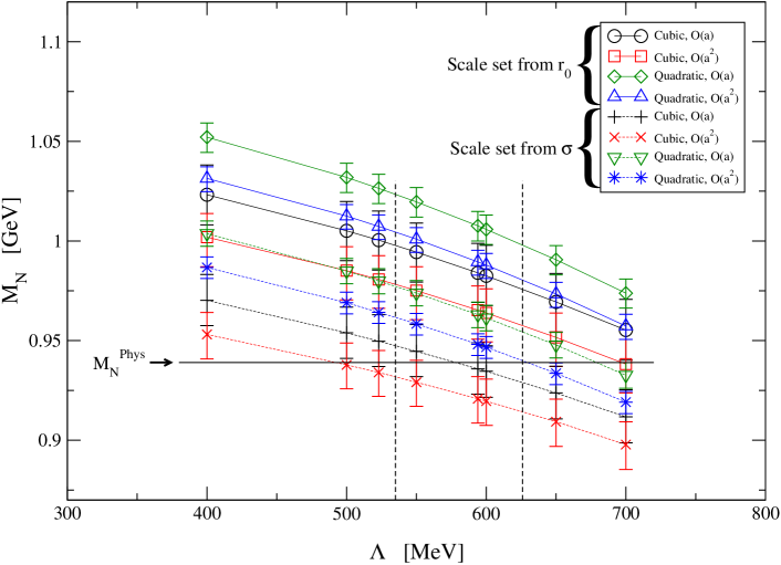
Figure 6.20: A plot of $M_{N}$ as a function of $\Lambda$ from the Adelaide approach using a dipole form factor. Recall that the best $\Lambda$ value when the scale is set from $r_{0}(\sigma)$ for the dipole form factor is $\Lambda=594(523)$ MeV. The two vertical dashed lines define the range of acceptable $\Lambda$ values (535 MeV $\leq\Lambda\leq$ 626 MeV) obtained by increasing $\chi^{2}$ by unity in fig. 6.13.

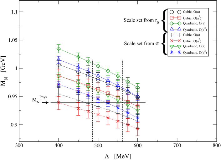
Figure 6.21: A plot of $M_{N}$ as a function of $\Lambda$ from the Adelaide approach using a Gaussian form factor. Recall that the best $\Lambda$ value when the scale is set from $r_{0}(\sigma)$ for the Gaussian form factor is $\Lambda=525(475)$ MeV. The two vertical dashed lines define the range of acceptable $\Lambda$ values (486 MeV $\leq\Lambda\leq$ 562 MeV) obtained by increasing $\chi^{2}$ by unity in fig. 6.14.

We summarise the results of this section which are outlined in table 6.6 and figures 6.20 and 6.21 below.

• The statistical errors in the mass estimates are typically less than 1% for the quadratic extrapolations and less than 2% for the cubic extrapolations.

• We see disagreement between all types of fit when different methods are used to set the scale. When the scale is set from $r_{0}$ the mass predictions are always higher than when the scale is set from $\sigma$. We observed a similar effect in the case of the of the mesons (5.9), although it is less pronounced.

• We also see that the mass predictions for a particular method (i.e. the Adelaide dipole, Adelaide Gaussian or naive method) have a variation in the results of between 3% and 5%, with the largest variation in the naive mass predictions. This disagreement suggests instability in the fits. We believe this is because the lattice systematics are more complicated than those we have uncovered.

• The Adelaide method always produces the mass prediction closest to the physical nucleon mass. For the cubic fits the Adelaide mass predictions are very accurate compared to their naive counterparts, they are typically within two statistical errors of the experimental mass. For the Adelaide method to reproduce the experimental mass prediction a rescaling of around 3% in $r_{0}$ and 1% in $\sqrt{\sigma}$ is needed.

• The variation of $M_{N}$ in the region of allowed values of $\Lambda$ is very small for each different fit. Typically of the order of the other uncertainties.

As with the results of the meson study (chap 5) we conclude by noting all of these points favour the Adelaide approach over the naive method. We believe that the Adelaide method should be the preferred method when performing chiral extrapolations and is a significant improvement over the naive method. To give the final value for $M_{N}$ for both the Adelaide method and the naive method, we use our preferred fitting function (the cubic with ${\cal O}(a^{2})$ corrections in $a_{0}$) and our preferred method for setting the scale (from $r_{0}$). For the Adelaide method we use our preferred form factor which is the dipole form factor. We quote an error that is based on the spread in the mass predictions (for the $r_{0}$ case only). We also (for the Adelaide method) include an estimate of the error associated with the $\Lambda$ parameter which is taken from the vertical dashed lines in figure 6.20.

Hence our final mass estimate for the nucleon is

$$M_{N}^{Adelaide} = 965(15){\scriptstyle{}^{+{41}}_{-{0}}}{\scriptstyle{}^{+{13}}_{-{8}}}\textrm{[MeV]}$$ (6.33)

$$M_{N}^{Naive} = 1023(15){\scriptstyle{}^{+{53}}_{-{0}}}\textrm{[MeV]}$$ (6.34)

where the first error is statistical and the second is taken from the fit procedure. The third error in the Adelaide case is that associated with the $\Lambda$ parameter. We have not considered any error that may be associated with the determination of $r_{0}$. We see that although the Adelaide prediction has a slightly wider error range, at its lower limit it comes within 3 [MeV] of the experimental value confirming the Adelaide method to be the better chiral extrapolation procedure.

6.6 Setting the scale

In this chapter we have studied two methods of setting the scale, from $r_{0}$ and from $\sigma$. We remind the reader of the results of section 5.5.1 where we investigated the ratio of these scales. When plotting $a_{\sigma}/a_{r_{0}}$ against $a_{r_{0}}$ we found that the plot had a roughly constant value of 5% above unity (fig 5.17). We suggested that an explanation for this could be if the ratio $\sqrt{\sigma}r_{0}=440$ [MeV] $\times~{}0.49$ [fm] is about 5% below its true value. This would explain why, when setting the scale from $r_{0}$, the estimates of the nucleon mass $(M_{N})$ are always larger than those where the scale if set from $\sigma$ (table 6.6) for the naive case. For the Adelaide method the relationship between the lattice scale $a^{-1}$ and $M_{N}$ is a highly non-linear one due to the functional form of $\Sigma_{TOT}$. So we cannot imfere a similar relationship between mass estimates from different methods used to set the scale as in the naive case. We also believe that this non-unit ratio is the cause of the difference in preferred values of $\Lambda$ that is observed when different methods are used to set the scale (figs 6.13 & 6.14).

6.7 Conclusions

We conclude by listing the results of our study.

• We have shown the Adelaide method to be a valid method for chiral extrapolations.

• We have applied the generalised Adelaide chiral ansatz for the nucleon to the “pseudo-quenched” case (i.e. when $\kappa_{\rm sea}\neq\kappa_{\rm val}$).

• We have tried to uncover unquenching effects in the data but found little evidence of this and have not managed to quantify them.

• We have tried to quantify the residual ${\cal O}(a)$ effects, but feel that we have not uncovered the full lattice spacing systematics.

• We have studied different fitting approaches (secs 6.4.2 & 6.4.3) and found that our global procedure to be the more robust method.

• We have demonstrated the Adelaide method can predict a preferred value of the $\Lambda$ parameter with resulting errors approximately equal to other statistical errors in the procedure.

• We have shown the Adelaide method can predict a preferred functional form. By altering the $\Lambda$ parameter the Adelaide method causes the form factor to describe continuum physics as best it can.

• We have listed 24 different predictions for the nucleon mass (sec 6.6). We find the Adelaide method with a dipole form factor using a cubic fit with ${\cal O}(a^{2})$ corrections in the $a_{0}$ coefficient to be the best fitting procedure.

• We have indicated that small errors in $r_{0}$ and $\sigma$ may cause incorrect central values for our mass estimates (sec 6.6).

• Finally we note that theoretically our fit procedure could be improved if $\Lambda$ and the physical mass splitting between the $\Delta$ and nucleon were allowed to be free parameters in our fit procedure. This would (in theory) give a accurate $\Lambda$ parameter and also allow the $\Delta$ mass to be determined. It may also be possible to use an iterative procedure whereby the results of a fit are used as the physical mass splitting in an attempt to produce a more accurate determination of the nucleon mass, this in turn would be used to produce a more accurate determination of the $\Delta$ mass, ad infinitum.

As in the mesonic case we haven’t modelled finite-size effects because we don’t have enough different volumes to do this. Also although we haven’t performed an infinite volume extrapolation finite volume effects are considered by the Adelaide method (eq 5.6) since the momentum integral is replaced by the appropriate kinetic sum.

Chapter 7 Conclusions

This thesis describes the results of investigations into chiral extrapolation procedures. Our research focused on two types of extrapolation procedure, namely the Adelaide method and a standard polynomial extrapolation procedure which we refer to as the naive method. These methods were used to produce physical mass predictions which were then compared to experimental results. In the mesonic case we also studied the $J$–parameter [21]

To do this we simulated data which was first produced by the CP-PACS collaboration [22]. In the case of the Adelaide method self energy values corresponding to the CP-PACS data set were calculated. Our research has been restricted to the “pseudo-quenched” case (i.e. when $\kappa_{\rm sea}\neq\kappa_{\rm val}$).

During our investigations we have

• quantified the residual ${\cal O}(a)$ effects in the CP-PACS data.

• introduced a global fitting method which allows us to treat data generated on lattices which have different lattice spacings as a single data set (for example sec 5.4.3).

• demonstrated how the Adelaide method can predict a preferred value for the $\Lambda$ parameter.

• indicated that small errors in the values of $r_{0}$ and $\sigma$ might be the cause of the slight inaccuracy in the central values of our mass estimates.

• studied different form factors and shown how the Adelaide method can pick a preferred function.

We now list our final results for studies of the $\rho$–mass, the nucleon mass and discuss the results for the $J$–parameter.

Our final result for the $\rho$–mass was obtained from the Adelaide method using our preferred fitting function (the quadratic fit with ${\cal O}(a^{2})$ corrections in the $a_{0}$ coefficient) and our preferred method for setting the scale (from $r_{0}$). We find

$$M_{\rho}^{Adelaide} = 779(4){\scriptstyle{}^{+{13}}_{-{0}}}{\scriptstyle{}^{+{5}}_{-{10}}}\textrm{[MeV]}$$ (7.1)

We remind the reader that the first error is a statistical error, the second is associated with the choice of fitting function and the third is that which is related to the determination of the $\Lambda$ parameter. The central value of our final estimate is just $9$ [MeV] away from the experimental value ($770$ [MeV]) and is equal to the experimental value within errors.

Our final result for the nucleon mass comes from the Adelaide method where we employ a dipole form factor, we use our preferred fitting function (for the nucleon this is the cubic with ${\cal O}(a^{2})$ corrections in $a_{0}$) and our preferred method for setting the scale (which is again from from $r_{0}$).

$$M_{N}^{Adelaide} = 965(15){\scriptstyle{}^{+{41}}_{-{0}}}{\scriptstyle{}^{+{13}}_{-{8}}}\textrm{[MeV]}$$ (7.2)

As with the $\rho$–mass prediction the first error is statistical, the second is taken from the fit procedure and the third error is that associated with the $\Lambda$ parameter. The nucleon mass prediction at its lower limit it comes within 3 [MeV] of the experimental value ($939$ [MeV])

In both cases we do not consider any error that may be associated with the determination of $r_{0}$.

For the $J$–parameter we study $J^{discrete}$. This is because $J^{discrete}$ can be easily be determined from experimental data, but $J$ itself cannot. We remind the reader that table 5.9 lists values for $J^{discrete}$. These values of $J^{discrete}$ are underestimates of the experimental value. This is a well known phenomena and is of no surprise.

We conclude this work by reiterating that the Adelaide method appears to be a valid chiral extrapolation procedure and should be favoured over standard polynomial fitting methods. We believe that for the foreseeable future the Adelaide method will prove to be a valuable tool for the extrapolation of lattice data. This is because it will be many years before high performance computers can run lattice simulations with quark masses near the chiral limit.

Bibliography

- [1] S. Sakata., 1956, Prog. Theor. Phys. 16, 686.
- [2] M. Ikeda, S. Ogawa, Y. Ohnuki., 1959, Prog. Theor. Phys. 22, 715.
- [3] M. Gell-Mann, Y. Ne’eman., 1964, The Eightfold Way. Reading: W. Benjamin.
- [4] K. Nishijima., 1955, Prog. Theor. Phys. 13, 285.
- [5] M. Gell-Mann., 1956, Nuovo. Cim. Supp. 4, 848.
- [6] M. Creutz., 1983, Quarks, gluons and lattices (Cambridge).
- [7] J. Smit., 2002, Introduction to Quantum Fields on a Lattice (Cambridge).
- [8] B. Efron., 1979, Bootstrap methods: another look at the jackknife, Ann. Stat. 29, 1-26.
- [9] M. Gell-Mann, M. Levy., 1960, Nuovo Cim. 16, 705.
- [10] J. Gasser, M. E. Sainio, A. Svarc., 1988, Nucl. Phys. B307, 779.
- [11] S. Weinberg., 1979, Physica 96A, 327.
- [12] R.D. Young, D.B. Leinweber, A.W. Thomas., 2003, Prog.Part.Nucl.Phys. 50 399-417. hep-lat/0212031
- [13] B. Holstein., Chiral Perturbation Theory: A Primer. hep-ph/9510344.
- [14] B. Borasoy., 1999, Phys.Rev. D59, 054021.
- [15] E. Jenkins & A. V. Manohar, Phys.Lett. B255, (1991) 558.
- [16] S. Scherer., Introduction to Chiral Perturbation Theory. hep-ph/0210398.
- [17] J. N. Labrenz & S. R. Sharpe., Phys.Rev. D54, (1996) 4595. hep-lat/9605034
- [18] C.K. Chow and S.J. Rey., 1998, Nucl.Phys. B528, 303. hep-ph/9708432.
- [19] V. Bernard, N. Kaiser, Ulf-G. Meißner., Chiral Dynamics in Nucleons and Nuclei. hep-ph/9501384.
- [20] Craig McNeile., Meson and Baryon Spectroscopy on a Lattice. hep-lat/0307027
- [21] R. Sommer., 1994, Nucl. Phys. B411, 839. hep-lat/9310022.
- [22] CP-PACS Collaboration, A.A. Khan et al., 2002, Phys.Rev. D65 054505. hep-lat/0105015.
- [23] CP-PACS Collaboration, S. Aoki et al., 1999, Phys.Rev. D60 114508. hep-lat/9902018.
- [24] D.B. Leinweber et al., 2001, Phys.Rev. D64 094502. hep-lat/0104013.
- [25] C.R.Allton, V.Gimenez, L.Giusti, F.Rapuano., 1997, Nucl.Phys. B489 427-452. hep-lat/9611021.
- [26] UKQCD Collaboration: C.R. Allton, et al., 2002, Phys.Rev. D65 054502. hep-lat/0107021.
- [27] UKQCD Collaboration, P. Lacock and C. Michael., 1995, Phys. Rev. D52 5213. hep-lat/9506009.
- [28] R. D. Young, D. B. Leinweber, A. W. Thomas., private communication.
- [29] R. D. Young, D. B. Leinweber, A. W. Thomas, S. V. Wright., 2002, Phys.Rev., D66 094507. hep-lat/0205017.
- [30] D. B. Leinweber, A. W. Thomas, K. Tsushima, S. V. Wright., 2000, Phys.Rev. D61 074502. hep-lat/9906027.
- [31] Malcolm Butler, Martin Savage, Roxanne Springer., 1993, Nucl.Phys. B399 69-88. hep-ph/9211247.
- [32] W. Armour, C. R. Allton, D. B. Leinweber, A. W. Thomas, R. D. Young., hep-lat/0510078
- [33] Particle Data Group., http://pdg.lbl.gov