Quantum fluctuations of k-strings: A case study.

Abstract:

K strings in Yang-Mills theory can be considered as bound states of $k$ elementary confining strings carrying one unit of colour flux. Current estimates of k-string tension $\sigma_{k}$ are very sensitive to the leading corrections due to quantum fluctuations of the string. In this study we address this problem by comparing Polyakov-Polyakov correlators in the fundamental representation ($k=1$) with the corresponding ones with $k=2$ in the confining phase of a ${\mathbb{Z}}_{4}$ gauge theory in three dimensions. Highly efficient simulation techniques are available in this case. Although the $k=1$ Polyakov-Polyakov correlator matches nicely with the expected bosonic string effects up to the Next-to-Leading-Order, the $k=2$ Polyakov-Polyakov correlators show large deviations. This is an important source of potential systematic errors in the current estimates of $\sigma_{k}$.

1 Introduction

Significant effort has been invested recently in studies of the flux tubes induced by color sources in higher representations of $SU(N)$, built up of $j$ copies of quarks in the fundamental representation. The long-distance properties of the flux tube should depend only on its $N-$ality $k\equiv j\,({\rm mod}\,N)$, since all representations with the same $k$ can be converted into each other by the emission of an appropriate number of soft gluons. As a consequence, the heavier strings of given $N$-ality $k$ are expected to decay into the string with smallest string tension. The corresponding string is usually referred to as a $k$-string. If its tension $\sigma_{k}$ for any allowed $k$ satisfies the inequality $\sigma_{k_{1}+k_{2}}<\sigma_{k_{1}}+\sigma_{k_{2}}$, the $k-$string is stable against decay into two strings of lower $N$-ality.

Stable $k$ strings are expected to belong to the antisymmetric representation with $k$ quarks. This fact can be simply understood in terms of Casimir scaling, i.e. the hypothesis that the string tension for a given representation is proportional to the quadratic Casimir operator [1, 2]: within the set of all representations of $N-$ality $k$ the antisymmetric one corresponds to the minimum of the Casimir eigenvalues, suggesting

$$\sigma_{k}^{(c)}=\sigma\frac{k(N-k)}{N-1}~{}.$$ (1)

Another competing hypothesis is the sine law:

$$\sigma_{k}^{(s)}=\sigma\frac{\sin(k\pi/N)}{\sin(\pi/N)}~{},$$ (2)

which has been derived in the large $N$ limit of ${\cal N}=2$ supersymmetric $SU(N)$ gauge theory softly broken to ${\cal N}=1$ [3], in the M theory description of ${\cal N}=1$ supersymmetric $SU(N)$ gauge theory [4] and, more recently, in the AdS/CFT correspondence [5]. In some cases this formula is expected to be exact, while in others the calculated values of $\sigma_{k}$ turn out to be slightly smaller than $\sigma_{k}^{(s)}$.

Lattice calculations in pure $SU(N)$ gauge models for $N=6$ [6] and $N=4,5,6,8$ [7, 8] in $D=3+1$ point to the $k-$string tensions lying partway between the Casimir scaling and the sine law, however there is no complete consensus and some dedicated studies favour the sine formula [9].

These calculations extract the string tensions $\sigma_{k}$ from Polyakov correlators at a finite temperature $T$ assuming the free string prediction [10]

$$\sigma_{k}(T)=\sigma_{k}-\frac{(D-2)\pi T^{2}}{6}+O(T^{4})~{},$$ (3)

There is good evidence that this is a very accurate approximation to $k=1$ strings in all confining gauge theories irrespective of the gauge group once $T$ is small enough [6, 11, 12], but there is no evidence that this can be also extended for $k>1$. Actually we show in this work that for $k>1$ Eq.(3) is not adequate and needs corrections.

Our starting point was the observation that the effective string description, at least in the case $k=1$, is believed to be universal, that is to hold for all confining gauge theories. On the other hand in order to check the validity of Eq.(3) it is important to do a much more accurate finite volume study than any currently available for $SU(N)$ $k-$strings. Hence we decided to study a three-dimensional ${\mathbb{Z}}_{4}$ gauge theory, which is the simplest model supporting a $k=2$ string. Using a duality transformation it is possible to map this model into the symmetric Ashkin-Teller (AT) model, where very high precision can be achieved on large lattices, through a non-local cluster algorithm. The outcome of this analysis is uncontroversial: though at low temperature the tension of the fundamental string fits nicely with Eq.(3) even at Next-to-Leading-Order (NLO), we find a clear mismatch for the 2-string in the same temperature range, suggesting the need of corrections to Eq.(3).

Theoretically, there is something one can say about the origin of these corrections. $k-$strings can be viewed as bound states of $k$ fundamental strings. Accordingly, we expect that besides the mechanical vibration modes whose quantum contributions yield exactly Eq.(3), there should be breathing modes related to the internal degrees of freedom of the $k$ constituent strings.

2 The effective string model

The infrared description of any confining gauge theory is well described by an effective string model. A particularly simple string action is the Nambu-Goto one, where the correlation function of two Polyakov loops at a temperature $T=1/L$ and at a distance $R$ can be calculated at the NLO [13, 14], yielding

$$\langle P(0)\,P^{\dagger}(R)\rangle\propto\frac{{\rm e}^{-cL-\sigma\,RL+\frac{(D-2)\pi^{2}L\,E(\tau)}{1152\sigma\,R^{3}}+O(1/R^{5})}}{\eta(\tau)^{D-2}}~{};~{}\tau\equiv\frac{iL}{2R}~{};~{}E=2E_{4}-E^{2}_{2}~{},$$ (4)

where $\eta$ is the Dedekind eta function and $E_{n}(\tau)$ are the Eisenstein functions (see e.g. [14] for detailed definitions). There is strong evidence that at this order this formula is universal, i.e. it holds in whatever confining gauge theory [15, 16, 17].

3 Algorithm

We work directly in the dual form of the $3d\,{\mathbb{Z}}_{4}$ gauge model, i.e. a symmetric Ashkin-Teller (AT) model. It is described in terms of two coupled, ferromagnetic, Ising systems through the two-parameter action

$$S=-\sum_{\langle xy\rangle}\beta\ (\sigma_{x}\sigma_{y}+\tau_{x}\tau_{y})+\alpha\ \sigma_{x}\sigma_{y}\tau_{x}\tau_{y},$$ (5)

where $\sigma_{x}$ and $\tau_{x}$ are the Ising variables ($\sigma_{x},\tau_{x}=\pm 1$). The global ${\mathbb{Z}}_{4}$ symmetry of the action is generated by the transformation $\sigma\rightarrow-\tau,\ \tau\rightarrow\sigma$. An independent ${\mathbb{Z}}_{2}$ symmetry is generated by the transformation $\sigma\leftrightarrow\tau$, which is related to the charge conjugation of the corresponding dual model.

The great advantage of studying the $3d$ AT model instead of the original $3d\,{\mathbb{Z}}_{4}$ gauge theory is that a non-local cluster updating algorithm [18] can be used. Of course, in the AT model we have two spin variables, so it is necessary to extend the original method. The idea is the following: we take the two site variables $\sigma$ and $\tau$ as if they belonged to two distinct lattices $R_{\sigma}$ and $R_{\tau}$; we freeze the lattice $R_{\sigma}$ and apply the Swendsen-Wang algorithm to the variables $\tau$ so obtaining a new lattice $R^{\prime}_{\tau}$. At this point we freeze the lattice $R^{\prime}_{\tau}$ and we update the variables $\sigma$, and so on.

It is possible to show that in this statistical system the expectation value of the Wilson loop of the gauge model $\langle W_{\gamma}\rangle_{gauge}$ is given by:

$$\langle W_{\gamma}\rangle_{gauge}=\frac{Z^{*}_{AT}}{Z_{AT}},$$

where $Z_{AT}$ is the partition function of the AT model and $Z^{*}_{AT}$ is that modified by a suitable twist of the couplings. In particular, in order to determine the $\langle W_{\gamma}\rangle_{gauge}$ in the fundamental representation $(k=1)$ it suffices to flip the couplings of $\sigma$ or $\tau$ just in the links orthogonal to an arbitrary surface $\Sigma$ encircled by $\gamma=\partial\,\Sigma$. Similarly, flipping the signs of both couplings of $\sigma$ and $\tau$ in the same surface, we get the Wilson loop in the $k=2$ representation.

Actually, since we have a model written in terms of Ising variables we can use a very powerful method to estimate the expectation value of the Wilson loop based only on the topological linking properties of the Fortuin-Kasteleyn (FK) clusters [19]. For each FK configuration one looks for paths in the clusters and then applies the following rule:

• $W_{\gamma}=1$ if there is no path linked with the loop $\gamma$ or if the winding number modulo 2 is zero,

• $W_{\gamma}=0$ otherwise.

Note that using such a definition, the value of $W_{\gamma}$ does not change if dangling ends or bridges between closed path are added or removed [20].

In the AT model we apply the above rules separately for the two variables $\sigma$ and $\tau$, therefore we have, for each configuration, a value $W^{\sigma}$ and a value $W^{\tau}$, each of them corresponds to the value of the Wilson loop in the fundamental representation; the product $W^{\sigma}W^{\tau}$ corresponds to the value of Wilson loop in the $k=2$ representation.

The same ideas do apply to measure the Polyakov-Polyakov correlator $\langle P(0)P^{\dagger}(R)\rangle$.

4 Numerical results

In this paper we discuss data obtained by simulating the AT model in one point of the parameter space $(\alpha=0.05,\beta=0.207)$, where our best estimate for string tensions are $\sigma_{1}=0.02084(5)$ and $\sigma_{2}=0.0323(5)$. In this case, the tension ratio is $\sigma_{2}/\sigma_{1}\simeq 1.55$, while the values predicted by the sine or Casimir scaling for $N=4$ and $k=2$ are $\sqrt{2}\simeq 1.41$ and $4/3$, respectively.

We performed $10^{6}$ measurements for both $\sigma_{1}$ and $\sigma_{2}$ on a lattice $64^{2}\times L$. The value of $L$ has been determined in such a way that $T\simeq T_{c}/2$ using the relation $T_{c}/\sqrt{\sigma}\simeq 1.1$.

In order to check whether the functional relation (4) is an accurate description of the Polyakov-Polyakov correlator two conditions are needed: the fitting parameters (in particular $\sigma_{k}$) should be stable at large $R$ and the estimated value of $\sigma_{k}$ should not depend on $T$ since Eq.(4) should account for the $T$ dependence.

In Fig. 1a it is possible to see the $\sigma_{f}$ value fitted by the Leading-Order (LO) approximation (i.e. neglecting the $E$ term in (4)) in a range $[R_{min},18]$ (where $R_{min}$ is the value that appears on the x-axes); albeit for large values of $R_{min}$ it seems to appear a plateau, there are three different values of $\sigma_{f}$, therefore the functional relation (FR) used is not sufficiently accurate to determine it.

Fig. 1b is similar to Fig. 1a, but in this case we have used the same FR to determine the value of $\sigma_{ff}$; also in this case we can apply the previous considerations and the FR is not correct.

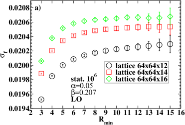
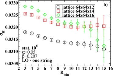
Figure 1: $\sigma_{f}$ and $\sigma_{ff}$ vs $R_{min}$ for three different $T$ at LO

Then, in Fig. 2, we fitted the value of $\sigma_{f}$ to two different FRs, one obtained by a LO approximation and the other one by NLO; the value of $\sigma_{f}$ increases significantly and the plateau appears for a smaller value of $R_{min}$.

In order to shed some light on the difficulty in determining a string tension that is free of systematic errors, in Fig. 3 we plot the values of $\chi^{2}/d.o.f.$ for fits which appear in Fig. 2; note that for $R_{min}\geq 11$ there is no difference in $\chi^{2}/d.o.f.$ between LO and NLO, even if the values of $\sigma_{f}$ in the same range (see Fig. 2) are different. It is interesting to note that in NLO case also the value of $\chi^{2}/d.o.f.$ shows a plateau for $R_{min}\geq 9$, therefore this FR better describes what happens at small values of $R$.

Fig. 4 is similar to Fig. 1a but now we use FRs obtained with a NLO approximation; now the FR is actually correct: the value of $\sigma_{f}$ is stable also for small values of $R_{min}$ and there is only one value of it for three different values of $L$ (i.e. different values of $T$).

Finally, in Fig. 5a and Fig. 5b we interpolate the value of $\sigma_{ff}$ with NLO approximation with two different hypotheses: in Fig. 5a the two strings are stuck together and fluctuate as a single string (we put D=3 in (4)); in Fig. 5b the two strings are assumed to fluctuate independently (this is equivalent to putting D=4 in (4)). It is clear that in this case the FR does not describe accurately $\sigma_{ff}$: in both cases a plateau does not appear for $\sigma_{ff}$ and there are different values for different values of $T$. This indicates that the current estimates of $\sigma_{k}$ are affected by systematic errors.

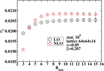
Figure 2: $\sigma_{f}$ vs $R_{min}$ for LO and NLO

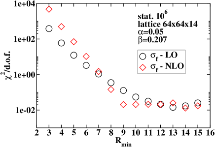
Figure 3: $\chi^{2}_{\sigma_{f}}/\mbox{d.o.f}$ vs $R_{min}$ for LO and NLO

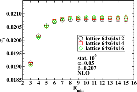
Figure 4: $\sigma_{f}$ vs $R_{min}$ for three different $T$ at NLO

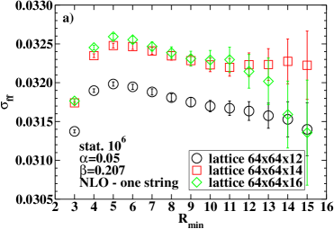
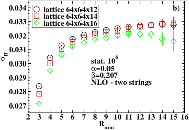
Figure 5: $\sigma_{ff}$ vs $R_{min}$ for three different $T$ at NLO: a) one string; b) two strings

5 Conclusions

The functional relations which are very accurate to fit data related to fundamental string tension are not adequate to describe 2-string tension.

An accurate estimate of the $k$-string tension is rather problematic: from a numerical point of view our analysis shows that a blind application of the usual formulas for the Polyakov-Polyakov correlators introduces strong systematic errors. From a theoretical point of view it is necessary to face the problem of determining the correct functional relation of Polyakov-Polyakov correlator for higher representations, which is presently unknown.

References

- [1] J. Ambjørn, P.Olesen and C. Peterson, Nucl. Phys. B 240 (1984) 186; Nucl. Phys. B 240 (1984) 533.
- [2] L. Del Debbio, M. Faber, J. Greensite and S. Olejnik, Phys. Rev. D 55 (1997) 2298 [hep-lat/9610005].
- [3] M.R. Douglas and S.H. Shenker, Nucl. Phys. B 481 (1995) 513 [hep-th/9503163].
- [4] A. Hanany, M.J. Strassler and A. Zaffaroni, Nucl. Phys. B 513 (1998) 87 [hep-th/9707244].
- [5] C.P. Herzog and I. R. Klebanov, Phys. Lett. B 526 (2002) 388 [hep-th/0111078].
- [6] L. Del Debbio, H. Panagopoulos, P. Rossi and E. Vicari, Phys. Rev. D 65 (2002) 021501 [hep-th/0106185].
- [7] B. Lucini and M. Teper, Phys. Rev. D 64 (2001) 105019 [hep-lat/0107007].
- [8] B. Lucini, M. Teper and U. Wengler, JHEP 0406 (2004) 012 [hep-lat/0404008].
- [9] L. Del Debbio, H. Panagopoulos, P. Rossi and E. Vicari, JHEP 01 (2002) 009 [hep-th/0111090]; hep-th/0409203.
- [10] M. Lüscher, K. Symanzik and P. Weisz, Nucl. Phys. B 173 (1980) 365.
- [11] M. Caselle, R. Fiore, F. Gliozzi, M. Hasenbusch and P. Provero, Nucl. Phys. B 486 (1997) 245 [hep-lat/9609041].
- [12] F. Gliozzi and P. Provero, Nucl. Phys. B 556 (1999) 76 [hep-lat/9903013].
- [13] K. Dietz and T. Filk, Phys. Rev. D 27 (1983) 2944.
- [14] M. Caselle, M. Hasenbusch and M. Panero, JHEP 0503 (2005) 026 [hep-lat/0501027].
- [15] M. Lüscher and P. Weisz, JHEP 0407 (2004) 014 [hep-th/0406205].
- [16] J. M. Drummond, hep-th/0411017.
- [17] N. D. H. Dass and P. Matlock, hep-th/0606265.
- [18] R. H. Swendsen and J. S. Wang, Phys. Rev. Lett. 58 (1987) 86.
- [19] F. Gliozzi and S. Vinti, Nucl. Phys. Proc. Suppl. 53 (1997) 593 [hep-lat/9609026].
- [20] F. Gliozzi, S. Lottini, M. Panero and A. Rago, Nucl. Phys. B 719 (2005) 255 [cond-mat/0502339].