HU–EP–06/27 The infrared behavior of lattice QCD Green’s functions
A numerical study of lattice QCD in Landau gauge
DISSERTATION
zur Erlangung des akademischen Grades
doctor rerum naturalium
(Dr. rer. nat.)
im Fach Physik
eingereicht an der
Mathematisch-Naturwissenschaftlichen Fakultät I
der Humboldt-Universität zu Berlin

Abstract

Within the framework of lattice QCD we investigate different aspects of QCD in Landau gauge using Monte Carlo simulations. In particular, we focus on the low momentum behavior of gluon and ghost propagators. The gauge group is that of QCD, namely $SU(3)$. For our study of the lattice gluodynamic, simulations were performed on several lattice sizes ranging from $12^{4}$ to $48^{4}$ at the three values of the inverse coupling constant $\beta=5.8$, 6.0 and 6.2.

Different systematic effects on the gluon and ghost propagators are studied. We demonstrate that the ghost dressing function systematically depends on the choice of Gribov copies at low momentum, while the influence on the gluon dressing function is not resolvable. Also the eigenvalue distribution of the Faddeev-Popov operator is sensitive to Gribov copies.

We show that the influence of dynamical Wilson fermions on the ghost propagator is negligible at the momenta available to us. For this we have used gauge configurations which were generated with two dynamical flavors of clover-improved Wilson fermions. On the contrary, fermions affect the gluon propagator at large and intermediate momenta, in particular where the gluon propagator exposes its characteristic enhancement compared to the free propagator.

We also analyze data for both propagators obtained on asymmetric lattices. By comparing these results with data obtained on symmetric lattices, we find that both the gluon and the ghost propagator suffer from systematic effects at the lowest on-axis momenta available on asymmetric lattices.

We compare our data with the infrared exponents predicted in studies of truncated systems of Dyson-Schwinger equations for the gluon and ghost propagators. We cannot confirm neither the values for both exponents nor the relation which is proposed to hold between them. In any case, we demonstrate that the infrared behavior of gluon and ghost propagators, as found in this thesis, is consistent with different criteria for confinement. In fact, we verify that our data of the ghost propagator and also of the Kugo-Ojima confinement parameter satisfy the Kugo-Ojima confinement criterion. The Gribov-Zwanziger horizon condition is satisfied by the ghost propagator. Also the gluon propagator seems to vanish in the zero-momentum limit. However, we cannot judge without doubt on the existence of an infrared vanishing gluon propagator. Furthermore, explicit violation of reflection positivity by the transverse gluon propagator is shown for the quenched and unquenched case of $SU(3)$ gauge theory.

The running coupling constant given as a renormalization-group-invariant combination of the gluon and ghost dressing functions does not expose a finite infrared fixed point. Rather the data are in favor of an infrared vanishing coupling constant. This behavior does not change if the Gribov ambiguity or unquenching effects are taken into account. We also report on a first nonperturbative computation of the $SU(3)$ ghost-gluon-vertex renormalization constant. We find that it deviates only weakly from being constant in the momentum subtraction scheme considered here.

We present results of an investigation of the spectral properties of the Faddeev-Popov operator at $\beta=5.8$ and 6.2 using the lattice sizes $12^{4}$, $16^{4}$ and $24^{4}$. For this we have calculated the low-lying eigenvalues and eigenmodes of the Faddeev-Popov operator. The larger the volume the more eigenvalues are found accumulated close to zero. Using the eigenmodes for a spectral representation of the ghost propagator it turns out that for our smallest lattice only 200 eigenvalues and eigenmodes are sufficient to saturate the ghost propagator at lowest momentum. We associate exceptionally large values occurring occasionally in the Monte Carlo history of the ghost propagator at larger $\beta$ to extraordinary contributions of the low-lying eigenmodes.

Keywords:
Gluon and ghost propagators, lattice QCD, Landau gauge, confinement

Abstract

Diese Arbeit untersucht im Rahmen der Gittereichtheorie verschiedene Aspekte der QCD in der Landau-Eichung, insbesondere solche, die mit den Gluon- und Geist-Propagatoren zusammenhängen. Die Eichgruppe ist die der QCD, $SU(3)$, und wir untersuchen die Propagatoren bei kleinen Impulsen. Für unsere Untersuchungen der reinen Gluodynamik haben wir zahlreiche Monte-Carlo Simulationen auf diversen Gittergrössen durchgeführt. Die Gittergrössen variieren im Bereich von $12^{4}$ bis $48^{4}$. Als inverse Kopplungskonstanten haben wir die Werte $\beta=5.8$, 6.0 und 6.2 gewählt.

Wir analysieren den Einfluss unterschiedlicher systematischer Effekte auf das Niedrigimpulsverhalten der Gluon- und Geist-Propagatoren. Wir zeigen, dass der Formfaktor des Geist-Propagators bei kleinen Impulsen systematisch von der Wahl der Eichkopien (Gribov-Kopien) abhängt. Hingegen können wir einen solchen Einfluss auf den Gluon-Propagator nicht feststellen. Ebenfalls wird die Verteilung der kleinsten Eigenwerte des Faddeev-Popov-Operators durch die Wahl der Gribov-Kopien beeinflusst.

Wir zeigen außerdem, dass der Einfluss dynamischer Wilson-Fermionen auf den Geist-Propagator für die untersuchten Impulse vernachlässigbar ist. Dazu haben wir Eichkonfigurationen betrachtet, die mit einer $N_{f}=2$ clover-verbesserten Wirkung erzeugt worden sind. Für den Gluon-Propagator können wir jedoch einen deutlichen Einfluss für große und mittlere Impulse feststellen, insbesondere in dem Impulsbereich, wo der Gluon-Propagator im Vergleich zum freien Fall seine charakteristische Erhöhung aufweist.

Zusätzlich wurden beide Propagatoren auf asymmetrischen Gittern gemessen. Der Vergleich dieser Daten mit denen, die auf symmetrischen Gittern gewonnen wurden, zeigt, dass die Asymmetrie deutliche systematische Effekte im Bereich kleiner Impulse verursacht. Besonders deutlich wird das für die Daten, die bei Impulsen in Richtung der elongierten Gitterlänge gemessen worden sind.

Weiterhin vergleichen wir unsere Daten mit den Infrarot-Exponenten, die in Studien von abgeschnittenen (truncated) Systemen von Dyson-Schwinger-Gleichungen für den Gluon- und Geist-Propagator vorhergesagt wurden. Im Rahmen unserer Messungen können wir weder die Werte der Exponenten noch die vorhergesagte Beziehung zwischen beiden bestätigen. In jedem Falle können wir aber zeigen, dass das in dieser Arbeit gefundene Niedrigimpulsverhalten im Einklang mit verschiedenen Kriterien für Confinement (Einschluss von Farbladungen) ist. Wir zeigen, dass unsere Daten sowohl für den Geist-Propagator als auch für den Kugo-Ojima-Confinement-Parameter das Kugo-Ojima-Confinement-Kriterium erfüllen. Außerdem ist die Gribov-Zwanziger-Horizontbedingung für den Geist-Propagator erfüllt. Der Gluon-Propagator scheint im Grenzfall verschwindender Impulse zu Null zu streben. Dennoch können wir nicht endgültig darüber urteilen, ob dies der Fall ist. Wir zeigen zusätzlich, dass der transversale Gluon-Propagator explizit die Reflektions-Positivität verletzt. Das gilt sowohl mit als auch ohne den Einfluss dynamischer Fermionen.

Wir berechnen die laufende (effektive) Kopplung, die sich als eine renormierungsgruppeninvariante Kombination der Gluon- und Geist-Formfaktoren ergibt. Unsere Ergebnisse zeigen deutlich, dass im Bereich kleiner Impulse die laufende Kopplung kleiner wird und so vermutlich kein endlicher Infrarot-Fixpunkt im Grenzfall Impuls Null angestrebt wird. Dieses Verhalten ist unabhängig vom Einfluss der Gribov-Kopien oder von der Hinzunahme dynamischer Fermionen. Wir präsentieren außerdem eine erste nichtstörungstheoretische Berechnung der Renormierungskonstante des $SU(3)$ Ghost-Gluon-Vertex. Wir zeigen, dass in dem untersuchten Renormierungsschema keine wesentliche Abweichung von einem konstanten Verhalten gefunden wird.

Wir berichten außerdem über Untersuchungen zu spektralen Eigenschaften des Faddeev-Popov-Operators bei $\beta=5.8$ and 6.2. Dazu haben wir eine Reihe der kleinsten Eigenwerte und Eigenvektoren dieses Operators auf den Gittergrößen $12^{4}$, $16^{4}$ und $24^{4}$ berechnet. Wir sehen, dass sich umso mehr Eigenwerte nahe Null konzentrieren, je größer das physikalische Volumen ist. Anhand einer spektralen Entwicklung des Geist-Propagators können wir zeigen, dass für unser kleinstes Gitter ca. 200 Eigenwerte und Eigenvektoren genügen, um den Wert des Geist-Propagators beim kleinsten Impuls zu reproduzieren.

Wir zeigen ferner, dass die selten auftretenden, exzeptionell großen Messwerte, die für den Geist-Propagator im Verlauf der Monte-Carlo Simulation bei größeren $\beta$ Werten gefunden werden, durch außerordentlich starke Beiträge der niedrigsten Eigenmoden zu den entsprechenden Fourierkomponenten hervorgerufen werden. Schlagwörter:
Gluon- und Geist-Propagatoren, Gitter-QCD, Landau-Eichung, Confinement

This Ph.D. thesis has been submitted to the Humboldt-University Berlin on May 3rd, 2006. It has been successfully defended on July 18th, 2006. The accepted official version is available online from the ’Dokumenten- und Publikationsserver’ (http://edoc.hu-berlin.de) of the Humboldt-University Berlin. Part of chapter 4 has been published in Ref. SIMPS05d and chapter 6 is based on Ref. SIMP [06]. All results presented in this thesis represent the research status of May 2006.

Contents

1. ‣ HU–EP–06/27 The infrared behavior of lattice QCD Green’s functions A numerical study of lattice QCD in Landau gauge DISSERTATION zur Erlangung des akademischen Grades doctor rerum naturalium (Dr. rer. nat.) im Fach Physik eingereicht an der Mathematisch-Naturwissenschaftlichen Fakultät I der Humboldt-Universität zu Berlin
3. 1 The various colors of QCD
   1. 1.1 Quantization of QCD
      1. 1.1.1 The classical QCD Lagrangian
      2. 1.1.2 Functional-integral quantization of QCD
      3. 1.1.3 The Faddeev-Popov method
      4. 1.1.4 An effective Lagrangian density in covariant gauge
      5. 1.1.5 The BRST formalism
   2. 1.2 Regularization and renormalization
      1. 1.2.1 Regularization
      2. 1.2.2 Renormalization
      3. 1.2.3 The MOM scheme
   3. 1.3 The renormalization group
      1. 1.3.1 The renormalization group equation
      2. 1.3.2 Perturbative expansion of the $\beta$–function
      3. 1.3.3 The running coupling constant
      4. 1.3.4 The anomalous dimension
4. 2 Infrared QCD and criteria for confinement
   1. 2.1 Nonperturbative approaches to QCD
      1. 2.1.1 Brief remarks on nonperturbative methods
      2. 2.1.2 The problem of Gribov copies
      3. 2.1.3 Nonperturbative quantization in Landau gauge
   2. 2.2 The Dyson Schwinger equations of QCD
      1. 2.2.1 Infrared behavior of ghost and gluon propagators in Landau gauge
      2. 2.2.2 A nonperturbative running coupling constant
      3. 2.2.3 The finiteness of the ghost-gluon vertex
   3. 2.3 Criteria for confinement in linear covariant gauges
      1. 2.3.1 The Kugo–Ojima confinement scenario
      2. 2.3.2 The Gribov–Zwanziger horizon condition
      3. 2.3.3 Violation of reflection positivity as a criterion for confinement
5. 3 QCD Green’s functions in lattice Landau gauge
   1. 3.1 Basics of lattice QCD
      1. 3.1.1 The lattice and its fields
      2. 3.1.2 The Wilson action with clover-improved fermions
      3. 3.1.3 Vacuum expectation values from MC simulations
   2. 3.2 The Landau gauge on the lattice
      1. 3.2.1 The gauge functional
      2. 3.2.2 The Faddeev-Popov operator
      3. 3.2.3 Defining $\Gamma$, $\Omega$ and $\Lambda$ on the lattice
   3. 3.3 Lattice definition of our observables
      1. 3.3.1 The (inverse) FP operator in momentum space
      2. 3.3.2 The gluon and ghost propagator
      3. 3.3.3 The Kugo-Ojima confinement parameter
      4. 3.3.4 Renormalization of propagators
      5. 3.3.5 The ghost-gluon-vertex renormalization constant
6. 4 Results for lattice QCD Green’s functions
   1. 4.1 General prerequisites
      1. 4.1.1 Specification of our lattice samples
      2. 4.1.2 Gauge–fixing
      3. 4.1.3 The fc-bc strategy
      4. 4.1.4 Selection of momenta
      5. 4.1.5 Mapping to physical units
   2. 4.2 Systematic effects on gluon and ghost propagators at low momentum
      1. 4.2.1 Finite volume and discretization effects
      2. 4.2.2 Asymmetric lattices cause strong systematic errors
      3. 4.2.3 Facing the problem of Gribov copies
   3. 4.3 The infrared behavior of gluon and ghost propagator in the quenched and unquenched case
      1. 4.3.1 The gluon propagator
      2. 4.3.2 The ghost propagator
   4. 4.4 The running coupling and the ghost-gluon vertex
      1. 4.4.1 Results for the running coupling constant
      2. 4.4.2 The vertex renormalization constant
7. 5 Confinement criteria under the lattice microscope
   1. 5.1 Is the Gribov-Zwanziger horizon condition satisfied?
   2. 5.2 The Kugo-Ojima confinement parameter
      1. 5.2.1 Expected infrared behavior
      2. 5.2.2 Explicit lattice data for the function $u(q^{2})$
   3. 5.3 The gluon propagator explicitly violates reflection positivity
8. 6 Spectral properties of the FP operator
   1. 6.1 Specification of lattice samples
   2. 6.2 The low-lying eigenvalue spectrum
      1. 6.2.1 The lowest and second lowest eigenvalues
      2. 6.2.2 An estimate for the density of low-lying eigenvalues
   3. 6.3 Eigenmode expansion of the ghost propagator
   4. 6.4 The problem of exceptional configurations
   5. 6.5 Localization properties of low-lying eigenvectors
9. ‣ HU–EP–06/27 The infrared behavior of lattice QCD Green’s functions A numerical study of lattice QCD in Landau gauge DISSERTATION zur Erlangung des akademischen Grades doctor rerum naturalium (Dr. rer. nat.) im Fach Physik eingereicht an der Mathematisch-Naturwissenschaftlichen Fakultät I der Humboldt-Universität zu Berlin
10. A Some details on algorithms and performance
    1. A.1 A note on the algorithms used
    2. A.2 Experience report on lattice Landau gauge fixing
       1. A.2.1 Over-relaxation versus Fourier–accelerated gauge-fixing
       2. A.2.2 A way to preselect best gauge copies
    3. A.3 Speeding up the inversion of the FP operator
11. Acknowledgments

[0,l,A,] t present we are reasonably confident that the physics of strong interaction, i.e. the rich field of hadron physics, is completely described by a quantized nonabelian gauge field theory which is based on the gauge group of $SU(3)$ color symmetry. This theory is called Quantum Chromodynamics (QCD). Its fundamental constituents are quarks and gluons. Quarks are spin 1/2 fermion fields carrying fractional electric charge and the gluons are nonabelian spin 1 gauge fields which interact with the quarks as well as among themselves. Due to its nonabelian nature the renormalization group tells us that QCD is asymptotically free at large Euclidean momentum. In this regime perturbative QCD is relevant and theoretical predictions have been successfully confronted with experiments. The experimental successes of QCD and the partial progress towards a full understanding of the theory form the basis for our present belief that QCD is the right theory describing all strong interaction physics.

Beyond perturbation theory, however, QCD is still not completely understood, even though — as far as we know — it is not in conflict with any existing phenomenology of the strong interaction. Note that in contrast to QED the elementary fields in QCD, the quarks and gluons, do not describe existing particles and thus a particle interpretation in QCD has to be completely divorced from its elementary degrees of freedom. According to QCD all strongly interacting particles, the hadrons, are colorless bound states of quarks. This phenomenon is called confinement, but the mechanism which confines quarks and gluons has to be established yet from first principles. Moreover, due to the complexity of QCD, a full description of hadronic states and processes directly in terms of QCD presents an exciting challenge since many years.

Many hadronic features have been investigated in the framework of phenomenological models (see e.g. VW [91]; Kle [92]; ERV [94]) which mimic the essential properties of QCD, namely asymptotic freedom at short distance and confinement at large distances. This approach represents a rather practical point of view and is sufficient if one is just interested in the effective theory of hadrons at low energies. But if QCD is the theory of strong interactions a coherent description directly based on the dynamics of confined quarks and gluons should be possible.

For such a description a complete picture for all propagators and vertex functions of QCD should be available. These Green’s functions may then serve as input into bound state calculations based on the Bethe-Salpeter equations for mesons or the Faddeev equations for baryons. But also from a purely theoretical point of view a consistent picture of all QCD Green’s functions is interesting. In particular, their infrared momentum behavior provides insight into the mechanism of quark and gluon confinement AvS [01]. To give just one example: The realization of the Kugo-Ojima confinement scenario KO [79]; Kug [95] in QCD in covariant gauges is encoded in the infrared behavior of the ghost 2-point function. Therefore, the investigation of QCD Green’s function at low momentum is important for a coherent description of hadronic states and processes and also for an understanding of confinement.

The infrared momentum region corresponds to strong coupling rather than weak coupling and hence perturbation theory is of no avail in studying QCD at low momentum. Genuinely nonperturbative approaches have to be used to explore QCD in this area. The Euclidean space, discretized, lattice gauge theory provides one possibility to study nonperturbative aspects of QCD by using Monte Carlo (MC) simulations. Another approach is given by solving truncated systems of the Dyson-Schwinger equations (DSEs) of QCD. The DSEs are infinite towers of coupled nonlinear integral equations relating different Green’s functions of QCD to each other. They are directly derived from a generating functional whose existence beyond perturbation theory still has to be assumed. In any case, studying DSEs involves the introduction of a gauge condition which is not necessary in the standard lattice approach to QCD.

DSE studies have been performed in recent years with growing intensity (see RW [94]; RS [00]; AvS [01]; MR [03] for an overview). In particular, for the case of Landau gauge it has been shown vSAH [97]; vSHA [98] that contributions of ghost fields are crucial for a consistent description of the infrared behavior of Landau gauge gluodynamics. In former studies Man [79]; ADJS [81]; AJS [82]; BP [89], ghost fields have always been neglected.

Different truncations have been employed since then to study the infrared behavior of gluon, ghost and quark propagators and the corresponding vertex functions. Truncations are essential to manage the infinite towers of DSEs. The solutions presented first in vSAH [97]; vSHA [98] and later in AB98a ; AB98b ; Blo [01, 02] and FAR [02]; FA [02]; Fis [03] all favor the picture of an infrared diverging ghost propagator being intimately connected with an infrared vanishing gluon propagator. In fact, both propagators are proposed to follow power laws at low momentum with intertwined infrared exponents LvS [02]; Zwa [02]. Such an infrared behavior is in agreement with the Gribov-Zwanziger horizon condition Gri [78]; Zwa [94, 02, 04] as well as with the Kugo-Ojima confinement criterion KO [79]; Kug [95]. Note that their satisfaction is crucial for the realization of confinement in QCD in Landau gauge. Unquenching effects on the infrared behavior are found to be small FA [03]. Moreover, dynamical chiral symmetry breaking and gluon confinement have been confirmed from solutions of truncated DSEs AvS [01]; FA [03]; ADFM [04].

Most of these DSE studies are done in Landau gauge. In this gauge, the ghost-gluon vertex was shown to not suffer from ultraviolet divergences at any order in perturbation theory Tay [71]; MP [78]. Assuming this to hold beyond perturbation theory, it allows for a definition of a nonperturbative running coupling constant that is solely given in terms of the gluon and ghost propagators and has a finite infrared fixed point, provided the mentioned infrared power laws hold vSAH [97]; vSHA [98]. In a recent DSE study AFLE [05] of vertex functions, the infrared fixed point has been confirmed, too. It has also been shown that this coupling constant enters directly the kernels of the DSEs for the gluon, ghost and quark propagators Blo [01, 02].

Even though Monte Carlo simulations of lattice QCD provide an alternative possibility to study QCD at a nonperturbative level, at present, they cannot compete with the DSE approach concerning the accessible region of low momenta. However, lattice QCD is a first principle approach to QCD that does not require us to “simplify” the theory. Unlike truncations of DSEs, the approximations involved in lattice QCD are systematically removable. This possibility of controlling the systematic errors makes this approach invaluable BHL⁺ [05]. Therefore, lattice simulations may provide an independent check whether the results obtained in the DSE approach are realized in lattice QCD, at least in the region of momenta available at present. Furthermore, lattice QCD enables us to study different models for confinement (see e.g. Gre [03]) by mutilating the theory such that confinement is explicitly lost. For example, removing vortices changes the infrared behavior of the lattice ghost propagator in Landau gauge such that it does not satisfy anymore aforementioned criteria for confinement GLR [04].

In recent years, different groups have investigated different aspects of lattice Landau gauge QCD. Some have studied the gauge group $SU(2)$, others $SU(3)$. In particular, the Adelaide Group has provided an impressive account on numerical data for the $SU(3)$ gluon LSWP [98, 99]; BBLW [00]; BBL⁺ [01] and quark propagators SW [01]; SLW [01]; BBL⁺ [02]; BHW [02]; ZBL⁺ [04]; Z⁺ [05]; B⁺05d ; P⁺ [06] and for the quark-gluon vertex SK [02]; SBK⁺ [03]. Their data are based on quenched and unquenched $SU(3)$ gauge configurations where the latter were generated with the AsqTad quark action by the MILC collaboration.

For the $SU(3)$ ghost propagator there were not so many data available until a few years ago, even though this propagator is expected to be related to the gluon propagator as mentioned above. The first lattice study of the $SU(2)$ and $SU(3)$ ghost propagators in Landau gauge was given in SS [96] and there were several studies in Landau gauge which have confirmed the anticipated behavior for the case of $SU(2)$ BCLM [04]; LRG [02]; GLR [04]; BCLM [03]. Similar investigations for the $SU(3)$ case at even lower momenta were not available at that time.

During the last three years, we have tried to bridge this gap by investigating the $SU(3)$ ghost and gluon propagators (and related objects) on quenched and unquenched $SU(3)$ gauge configurations. Our set of unquenched configurations were generated with clover-improved Wilson fermions by the QCDSF collaboration. We have found that for momenta lower than used in the $SU(2)$ studies (see above) qualitative differences to the anticipated infrared behavior of ghost and gluon propagators and of the running coupling constant appear.

At the same time other groups have performed similar investigations focussing on different interesting aspects. See, for example, FN04a ; FN04b ; FN05a ; FN06b ; FN06a for investigations of the gluon, ghost and quark propagators and of the running coupling constant using quenched and unquenched configurations (provided by the MILC collaboration). Studies of the $SU(3)$ gluon propagator at very low momentum can be found in OS05b ; SO05b ; OS05a ; SO05a . There the infrared exponent has been determined using lattices much elongated in time direction. A study of the $SU(3)$ ghost propagator at large momentum can be found in B⁺05c .

Furthermore, recent DSE studies FAR [02]; FA [02]; FGA [06]; FP [06] show that the infrared behavior of the gluon and ghost dressing functions and of the running coupling constant is changed on a torus. In particular, the running coupling decreases at low momenta. These findings agree with lattice data as shown in this thesis, but they contradict results obtained from DSE studies in the continuum. It is still unknown what is the reason for this disagreement. Note that a solution to this problem has been proposed in B⁺05b ; B⁺06a .

It is the intention of this thesis to give a summary of our results obtained within the last three years. Some were already published, others are just finished and being written up.

We have structured this thesis as follows: In the first chapter we introduce the path integral formulation of QCD and discuss the special problems related to the necessity of gauge fixing the action. A brief introduction to the BRST formalism is given and the renormalization program is recalled. In Chapt. 2 we discuss some aspects of nonperturbative QCD and introduce criteria for confinement which are available for QCD in Landau gauge. The lattice formulation of QCD in this gauge and a definition of all observables analyzed in this thesis is given in Chapt. 3. We present our results for the ghost and gluon propagators in Chapt. 4. Different systematic effects are analyzed and their influence on the infrared behavior of the gluon and ghost propagators is discussed. After this, we show that our data for both propagators satisfy necessary criteria for confinement. In Chapt. 6 spectral properties of the FP operator are analyzed. Finally, we draw our conclusions and give an outlook. The appendix contains some notes on algorithms and performance. In particular, we compare two popular gauge-fixing algorithms and show that the final ranking of gauge functional values is already visible at an intermediate iteration state. We also demonstrate how the inversion of the FP operator can be accelerated considerably.

Chapter 1 The various colors of QCD

[0,l,T,] his chapter briefly reviews the Euclidean formulation of QCD in the continuum, mainly in order to fix notations used subsequently. Starting with the classical Lagrangian density and its quantization, the problems encountered by fixing to covariant gauges are discussed. A short summary of the BRST formalism and renormalization is given.

1.1 Quantization of QCD

The success of quark-models in describing hadrons as bound states of quarks, but also of quark-parton models in deep-inelastic lepton-hadron scattering, to name but a few, suggests that the strong interaction should be described by a theory where the color symmetry of each quark flavor is a gauge symmetry and which is also asymptotically free at high energy-momentum transfers or short distances. Since asymptotic freedom is inherent in non-abelian gauge theories, and experiments like, for instances, the pion-decay $\pi^{0}\rightarrow 2\gamma$ suggest the gauge group to be $SU(3)$, we are reasonably confident at present that the strong interaction is completely described by a quantized non-Abelian gauge field theory based on the $SU(3)$ gauge group.

1.1.1 The classical QCD Lagrangian

A common way to setup a quantum field theory is to define first a Lagrangian density

$$\mathcal{L}\equiv\mathcal{L}[\Phi_{1}(x),\ldots,\Phi_{n}(x);\partial_{\mu}\Phi_{1}(x),\ldots,\partial_{\mu}\Phi_{n}(x)]$$ (1.1)

that is a functional of several fields $\Phi_{1}(x),\ldots,\Phi_{n}(x)$ and their derivatives necessary to host (in a consistent way) all the features and symmetries observed in experiments. This Lagrangian density or its space-time integral, the action

$$S[\Phi]\equiv\int d^{4}x\,\mathcal{L}\;,$$ (1.2)

is then used subsequently for a quantization of the theory choosing one of the well-known quantization methods, namely the Canonical operator formalism, the Stochastic formalism or the Functional-integral formalism Mut [98].

The most general form of the QCD Lagrangian density that not only accommodates all those mentioned properties of QCD, but also is renormalizable in any order of perturbation theory can be written (in Euclidean space) as

$$\mathcal{L}_{\textrm{inv}}=\frac{1}{4}F^{a}_{\mu\nu}F^{\mu\nu,a}-\bar{\psi}(\gamma_{\mu}D_{\mu}-m_{0})\psi\,.$$ (1.3)

Conceived in general terms, this Lagrangian density describes the interaction of the quark and antiquark fields, $\psi$ and $\bar{\psi}$, with the self-interacting gluon or gauge fields $A_{\mu}=A^{a}_{\mu}(x)T^{a}$. The latter are hidden in both the definition of the field-strength tensor

$$F^{a}_{\mu\nu}=\partial_{\mu}A^{a}_{\nu}-\partial_{\nu}A^{a}_{\mu}-\textsl{g}_{0}f^{abc}A^{b}_{\mu}A^{c}_{\nu}$$ (1.4)

(here in the adjoint representation, i.e. $a=1,\ldots,N_{c}^{2}-1$) and the covariant derivative

$$D^{kl}_{\mu}=\partial_{\mu}\delta^{kl}+i\textsl{g}_{0}A^{a}_{\mu}(T^{a})^{kl}$$ (1.5)

given in the fundamental representation (i.e. $k,l=1,\ldots,N_{c}$) of the Lie group $SU(N_{c}=3)$ with the eight hermitian generators $T^{a}$. Beside being hermitian, these generators satisfy $\operatorname{Tr}\big{(}T^{a}T^{b}\big{)}=\delta^{ab}/2$ and $[T^{a},T^{b}]=if^{abc}T^{c}$ where $f^{abc}$ are the structure constants of the Lie algebra $\mathfrak{su}(3)$. The bare coupling constant is labeled $\textsl{g}_{0}$. For the sake of completeness, we also remind on the covariant derivative in the adjoint representation:

$$D^{ab}_{\mu}=\partial_{\mu}\delta^{ab}+\textsl{g}_{0}f^{abc}A^{c}_{\mu}.$$ (1.6)

The quark fields

$$\psi\equiv\psi^{\alpha,l}_{f}(x)$$

and antiquark fields $\bar{\psi}\equiv\psi^{\dagger}\gamma_{0}$, of flavor $f=1,\ldots,N_{f}$ are anti-commuting spinor fields that transform under the fundamental representation of the $SU(N_{c}=3)$ color group, i.e. the color index runs over $l=1,\ldots,N_{c}$. The Dirac matrices $\gamma_{\mu}$ act upon the spinor indices $\alpha=1,\ldots,4$ of the quark fields. The bare mass $m_{0}$ is a free parameter (for each flavor) of the theory as is $\textsl{g}_{0}$.

By definition, the Lagrangian density in Eq. (1.3) is invariant under local $SU(3)$ gauge transformations

$$A_{\mu} \rightarrow \kern 1.00006pt\raise 4.30554pt\hbox{$\scriptstyle\omega$}\kern-1.99997ptA_{\mu}=g_{\omega}A_{\mu}g^{\dagger}_{\omega}+\frac{i}{\textsl{g}_{0}}\,g_{\omega}\partial_{\mu}g^{\dagger}_{\omega},$$ (1.7a)

$$\psi \rightarrow \;\kern 1.00006pt\raise 4.30554pt\hbox{$\scriptstyle\omega$}\kern-1.99997pt\psi=g_{\omega}\psi,$$ (1.7b)

$$\bar{\psi} \rightarrow \;\kern 1.00006pt\raise 4.30554pt\hbox{$\scriptstyle\omega$}\kern-1.99997pt\bar{\psi}=\bar{\psi}g^{\dagger}_{\omega}$$ (1.7c)

of gluon, quark and antiquark fields. Here $g_{\omega}$ is an element of the group $SU(3)$. It can be parameterized by a set of real-valued functions $\omega^{a}(x)$, i.e.

$$g_{\omega}\equiv g_{\omega}(x)=e^{-i\textsl{g}_{0}\cdot\omega^{a}(x)T^{a}}\quad\in SU(3).$$ (1.8)

In subsequent discussions we will frequently refer to the infinitesimal form of those local transformations. What is usually meant by that notion is the following. If the field $\Phi_{k}=\{\bar{\psi},\psi,A\}$ transforms under a local gauge transformation $\Phi_{k}\rightarrow\kern 1.00006pt\raise 4.30554pt\hbox{$\scriptstyle\omega$}\kern-1.99997pt\Phi_{k}$ as given in Eq. (1.7) then the corresponding infinitesimal transformation is defined by Col [84]:

$$\delta\Phi_{k}(x)\equiv\left.\omega^{b}\frac{\partial}{\partial\omega_{b}}\kern 1.00006pt\raise 4.30554pt\hbox{$\scriptstyle\omega$}\kern-1.99997pt\Phi_{k}\right|_{\omega=0}=\mathrel{\mathop{\mathchar 58\relax}}\omega^{b}\delta_{b}\Phi_{k}(x)\;.$$

Using Eq. (1.8) the infinitesimal local gauge transformations of the gluon and fermion fields take the form:

$$\delta_{\omega}A^{a}_{\mu} = \partial_{\mu}\omega^{a}+\textsl{g}_{0}f^{abc}\omega^{b}A^{c}_{\mu}\equiv D^{ab}_{\mu}\omega^{b}$$ (1.9a)

$$\delta_{\omega}\psi = -i\textsl{g}_{0}\omega^{a}T^{a}\psi$$ (1.9b)

$$\delta_{\omega}\bar{\psi} = +i\textsl{g}_{0}\omega^{a}\bar{\psi}T^{a}$$ (1.9c)

The invariance of the Lagrangian density $\mathcal{L}_{\textrm{inv}}$ under local gauge transformations, causes some extra difficulties for the quantization using either the functional-integral or the canonical formalism. For example, the definition of a functional-integral over gauge fields in the continuum requires a gauge condition to be introduced. As a consequence additional terms are added to $\mathcal{L}_{\textrm{inv}}$. In the resulting Lagrangian density, $\mathcal{L}_{\textrm{eff}}$, the gauge invariance is explicitly lost, but its particular form — it is BRST invariant (see below) — guarantees that expectation values of gauge-invariant observables are actually independent of the gauge condition used.

We note in passing that on the lattice such a gauge condition is superfluous, as long as gauge-invariant observables are studied. Therefore, the gauge-invariant action

$$S_{\textrm{inv}}=\int d^{4}x\;\mathcal{L}_{\textrm{inv}}$$ (1.10)

is sufficient for a lattice discretization. See Chapt. 3 for a particular lattice discretization as used in this study.

1.1.2 Functional-integral quantization of QCD

So far the theory is a classical field theory. To quantize it one chooses one of the well-known quantization methods, namely the Canonical operator formalism, the Stochastic formalism or the Functional-integral formalism. Indeed, all three methods should lead to the same physical predictions. However, the choice depends on the feasibility of the method for a particular topic.

A quantum field theory is completely characterized by the infinite hierarchy of $n$-point functions or Green’s functions. These are correlation functions of the fields $\Phi_{i}(x)$ and the three mentioned formalisms differ in how Green’s functions are calculated. For example, in the canonical approach the fields are regarded as operators for which canonical commutation relations hold. The Green’s functions are calculated as vacuum expectation values of time ordered products of those operators. The stochastic formalism introduced by Parisi and Wu PW [81] starts from the classical equation of motion. The fields are regarded as stochastic variables. See DH [87] for a comprehensive account on that subject.

The Functional-integral approach was introduced by Feynman Fey [48]. There the fields are taken to be c-numbers and the Lagrangian density takes its classical form. The Green’s functions are given by functional integrations of products of fields over all of their (weighted) possible functional forms. The present study focuses on the lattice regularization of QCD in Euclidean space. Since this approach relies on the functional integral formalism we demonstrate briefly the general concept.

Functional-integral formalism: Illustration of the general concept

The functional-integral formalism introduces generating functionals $Z$, $W$, and $\Gamma$ which generate, respectively, the full, connected and one-particle irreducible (1PI) Green’s functions. To get acquainted with the general concept let us assume that for the generic Lagrangian density (Eq. (1.1)) of $n$ different fields $\Phi_{i}$ the generating functional

$$Z[J]=\int[\mathcal{D}\Phi]\exp\left\{-\int d^{4}x\,\big{(}\mathcal{L}[\Phi(x)]+J^{a}_{i}(x)\Phi^{a}_{i}(x)\big{)}\right\}$$ (1.11)

for the full Green’s functions can be defined, i.e. there exist a well-defined measure $[\mathcal{D}\Phi]$. Then a full Green’s function $\langle\Phi^{a_{1}}_{1}(x_{1})\cdots\Phi^{a_{n}}_{n}(x_{n})\rangle$ is given by functional derivatives with respect to the sources $J^{a}_{i}(x)$, i.e.

$$\langle\Phi^{a_{1}}_{1}(x_{1})\cdots\Phi^{a_{n}}_{n}(x_{n})\rangle=\left.\frac{\delta^{n}Z[J]}{J^{a_{1}}_{1}(x_{1})\cdots J^{a_{n}}_{n}(x_{n})}\right|_{J^{a_{1}}_{1},\ldots,J^{a_{n}}_{n}=0}\;.$$

Together with Eq. (1.11) and the generic action $S[\Phi]$ (Eq. (1.2)) this yields

$$\langle\Phi^{a_{1}}_{1}(x_{1})\cdots\Phi^{a_{n}}_{n}(x_{n})\rangle=\frac{1}{Z[0]}\int[\mathcal{D}\Phi]\;\Phi^{a_{1}}_{1}(x_{1})\cdots\Phi^{a_{n}}_{n}(x_{n})\,e^{-S[\Phi]}\;.$$

Gauge orbits and gauge conditions

For a quantization of QCD within the functional formalism it is necessary to define the generating functional $Z[J]$ that generates all the Green’s functions of the theory. In particular, the definition of a path-integral over gluon fields needs special care, because it is ill-defined if done naively.

In fact, choosing a particular gauge field $\kern 1.00006pt\raise 4.30554pt\hbox{$\scriptstyle 0$}\kern-1.99997ptA_{\mu}(x)$ there are infinitely many others $\kern 1.00006pt\raise 4.30554pt\hbox{$\scriptstyle\omega$}\kern-1.99997ptA_{\mu}$ which are related to this by local gauge transformations as defined in Eq. (1.7a). The set of all those is usually referred to as the gauge orbit of $\kern 1.00006pt\raise 4.30554pt\hbox{$\scriptstyle 0$}\kern-1.99997ptA_{\mu}$, because each element $\kern 1.00006pt\raise 4.30554pt\hbox{$\scriptstyle\omega$}\kern-1.99997ptA_{\mu}$ in the orbit is obtained by acting upon $\kern 1.00006pt\raise 4.30554pt\hbox{$\scriptstyle 0$}\kern-1.99997ptA_{\mu}$ with a local gauge transformation $g_{\omega}(x)$. The Lagrangian $\mathcal{L}_{\textrm{inv}}$ is invariant under such a transformation by definition and so all (infinite) elements of one particular orbit give rise to the same value of $\mathcal{L}_{\textrm{inv}}$. This spoils a naive integration over all gluon fields, because an integral of kind

$$\int[DA]\;e^{-S_{\textrm{inv}}}=\int[D\kern 1.00006pt\raise 4.30554pt\hbox{$\scriptstyle 0$}\kern-1.99997ptA]\;e^{-S_{\textrm{inv}}}\int[D\omega]$$

is divergent. Here $S_{\textrm{inv}}$ denotes the action in Eq. (1.10), but for simplicity we have dropped fermionic fields. The integration over the gluon fields must be defined such that it restricts to gauge-inequivalent configurations, i.e. they must belong to different gauge orbits.

This can be achieved by choosing a gauge condition

$$\mathcal{F}[\kern 1.00006pt\raise 4.30554pt\hbox{$\scriptstyle\omega$}\kern-1.99997ptA;x]\Big{|}_{\omega=\bar{\omega}}=0$$ (1.12)

at each point $x$ in space-time. If this condition is satisfied for only one representative on each gauge orbit, i.e. the solution $\bar{\omega}$ is unique, then it is called an ideal gauge condition Wil [03]. The set of those representatives is called the fundamental modular region $\Lambda$. It is a hypersurface defined by Eq. (1.12) in the space of all gauge fields. If we can define an integration over this region, the integral

$$\int_{\Lambda}[DA]\;e^{-S_{\textrm{inv}}}$$

does not suffer from local gauge invariance, as does a naive integration.

If the gauge condition (Eq. (1.12)) is ambiguous, it is termed non-ideal and an integration beyond perturbation theory may become ill-defined. The different solutions to a non-ideal gauge condition belong to the same orbit and are called Gribov copies in honor of its discoverer Gri [78]. In the following, we assume the gauge condition to be ideal. Note that even popular non-ideal gauge conditions, like the Coulomb or Landau gauge, are sufficient within the framework of perturbation theory. This is because in perturbation theory only small fluctuations of $A^{a}_{\mu}(x)$ around zero are necessary and with respect to infinitesimal gauge transformations

$$g_{\omega}(x;\tau)=\mathbb{1}+i\tau\omega^{a}(x)T^{a}+O(\tau^{2})\qquad(\tau\ll 1).$$

even non-ideal gauge conditions are unique. The problems of Gribov copies and nonperturbative quantization will be discussed in Sec. 2.1.

1.1.3 The Faddeev-Popov method

From ordinary calculus of discrete $n$-dimensional vectors it is known that

$$1=\int\left[\prod^{n}_{i}df_{i}\right]\delta^{n}(\boldsymbol{f})=\int\left[\prod^{n}_{i}d\omega_{i}\right]\delta^{n}\left(\boldsymbol{f}(\boldsymbol{\omega})\right)\left|\det\frac{\partial f_{i}}{\partial\omega_{j}}\right|$$ (1.13)

where the determinant in the last expression is the Jacobian determinant that arise due to the substitution rule for integrals with multiple variables. If $f$ is invertible near $\omega$ then its Jacobian determinant at $\omega$ is non-zero (inverse function theorem).

If we assume in the following that Eq. (1.12) represents an ideal gauge condition, the identity Eq. (1.13) may be generalized to an identity for functional integrals

$$\mathbb{1}=\int[D\omega]\;\delta\left(\mathcal{F}[\kern 1.00006pt\raise 4.30554pt\hbox{$\scriptstyle\omega$}\kern-1.99997ptA]\right)\Delta_{\textrm{FP}}[A]$$ (1.14)

which was first proposed by Faddeev and Popov FP [67]. In this relation, the Jacobian determinant

$$\Delta_{\textrm{FP}}[A]\mathrel{\mathop{\mathchar 58\relax}}=\det M[A]$$ (1.15)

is known as the Faddeev-Popov (FP) determinant FP [67] of a matrix

$$M^{ab}_{xy}[A]\mathrel{\mathop{\mathchar 58\relax}}=\left.\frac{\delta\mathcal{F}[\kern 1.00006pt\raise 4.30554pt\hbox{$\scriptstyle\omega$}\kern-1.99997ptA^{a},x]}{\delta\omega^{b}(y)}\right|_{\omega=0}$$ (1.16)

that represents the change of $\mathcal{F}$ under local gauge transformation at $\omega=0$. Inserting the identity in Eq. (1.14) now in the naive integration over gluon fields we end up with

$$\int[DA]\;\Delta_{\textrm{FP}}[A]\;\delta(\mathcal{F}[A])\;e^{-S_{\textrm{inv}}[A]}.$$ (1.17)

This represents an integration over the fundamental modular region, but if and only if the gauge condition Eq. (1.12) is unique.

1.1.4 An effective Lagrangian density in covariant gauge

A popular gauge condition for practical calculations is given by the family of covariant gauges specified by the condition

$$\mathcal{F}^{a}[A]\mathrel{\mathop{\mathchar 58\relax}}=\partial_{\mu}A^{a}_{\mu}(x)-B^{a}(x)=0.$$ (1.18)

Here $B^{a}(x)$ is an arbitrary function. Since the work of Gribov Gri [78] it is well-known that local gauge conditions of this type are ambiguous with respect to finite gauge transformations (see also Sin [78]; Wil [03]), and so, in our notation, belongs to the class of non-ideal gauge conditions. With respect to infinitesimal gauge transformations, however, they are unique and may be treated as ideal ones.

The family of covariant gauges turns out to be useful in perturbative expansions in many applications. It also allows us to represent the delta function in the functional integral Eq. (1.17) as a (functional) integral over the fields $B$. Since these fields are arbitrary we can use a Gaussian weight of width $\xi_{0}$ to integrate over, i.e.

$$\int DB^{a}\;\exp\left\{-\frac{1}{2\xi_{0}}\int d^{4}x\;(B^{a})^{2}(x)\right\}\delta\left(\partial_{\mu}A^{a}_{\mu}(x)-B^{a}(x)\right)=\mathrel{\mathop{\mathchar 58\relax}}e^{-S_{\textrm{GF}}[A;\xi_{0}]}\;.$$

Here $S_{\textrm{GF}}[A;\xi_{0}]$ is defined as the (Euclidean) space-time integral of

$$\mathcal{L}_{\textrm{GF}}^{\xi}=\frac{1}{2\xi_{0}}\left[\partial_{\mu}A_{\mu}(x)\right]^{2}$$ (1.19)

$\mathcal{L}_{\textrm{GF}}^{\xi}$ is known as the gauge-fixing term which is added to the invariant Lagrangian density $\mathcal{L}_{\textrm{inv}}$. It serves as a substitute for the delta-function that specifies the hypersurface in the functional integral Eq. (1.17). The parameter $\xi_{0}$ is the gauge parameter that specifies the particular gauge condition in the family of covariant gauges. The special case of $\xi_{0}=0$ is known as the Landau or Lorentz gauge and $\xi_{0}=1$ as the Feynman gauge.

Never call a ghost stupid — A few good ghosts can help

Although the FP determinant (Eq. (1.15)) is not a local function of the gauge fields, the functional integration in Eq. (1.17) can be extended such that the FP determinant is expressed by an additional (local) term, $\mathcal{L}_{\textrm{FP}}$, added to $\mathcal{L}_{\textrm{inv}}$, too. This is done by the familiar device of integrating over ghost and anti-ghost fields $c$ and $\bar{c}$ which are independent Grassmann valued fields. With the definition of the FP matrix $M$ (Eq. (1.16)) we obtain in covariant gauge

$$M^{ab}_{xy}[A] = \left.\frac{\delta(\partial_{\mu}\kern 1.00006pt\raise 4.30554pt\hbox{$\scriptstyle\omega$}\kern-1.99997ptA^{a}_{\mu}(x)-B^{a}(x))}{\delta\omega^{b}(y)}\right|_{\omega=0}=\left.\partial^{x}_{\mu}\frac{\delta\kern 1.00006pt\raise 4.30554pt\hbox{$\scriptstyle\omega$}\kern-1.99997ptA^{a}_{\mu}(x)}{\delta\omega^{b}(y)}\right|_{\omega=0}$$ (1.20)

$$= -\partial^{x}_{\mu}D^{ab}_{x,\mu}[A]\delta^{4}(x-y)\;.$$

Here $D^{ab}_{x,\mu}$ denotes the covariant derivative in the adjoint representation. Using this, the term $\mathcal{L}_{\textrm{FP}}$, known as the ghost term, takes the form

$$\mathcal{L}_{\textrm{FP}}=-(\partial_{\mu}\bar{c}^{a})(\partial^{\mu}\delta^{ab}+\textsl{g}_{0}f^{abc}A^{c}_{\mu})c^{b}\;.$$ (1.21)

Generating functional for QCD in covariant gauge

In summary, we arrive at an effective Lagrangian density

$$\mathcal{L}_{\textrm{eff}}=\mathcal{L}_{\textrm{inv}}+\mathcal{L}_{\textrm{GF}}+\mathcal{L}_{\textrm{FP}}^{\xi}$$ (1.22)

where the individual terms $\mathcal{L}_{\textrm{inv}}$, $\mathcal{L}_{\textrm{GF}}$ and $\mathcal{L}_{\textrm{FP}}^{\xi}$ are defined in Eq. (1.3), (1.19) and (1.21), respectively. $\mathcal{L}_{\textrm{eff}}$ can be used to define the (Euclidean) generating functional (see e.g. AvS [01])

$$Z[j^{a},\bar{\eta},\eta, \sigma,\bar{\sigma}]=\int[\mathcal{D}A][\mathcal{D}\psi][\mathcal{D}\bar{\psi}][\mathcal{D}c][\mathcal{D}\bar{c}]$$

$$\cdot\exp\left\{-\int d^{4}x\;\left(\mathcal{L}_{\textrm{eff}}^{r}-A^{a}_{\mu}j^{a}_{\mu}-\bar{\eta}\psi-\bar{\psi}\eta-\bar{\sigma}c-\bar{c}\sigma\right)\right\}.$$ (1.23)

Here $\bar{\eta}$, $\eta$, $\sigma$ and $\bar{\sigma}$ refer to the Grassmannian sources, respectively, for the quark, anti-quark, ghost and anti-ghost fields as introduced above. In covariant perturbation theory this generating functional is used for the calculation of Euclidean Green’s functions as power series expansions of the interaction terms in $\mathcal{L}_{\textrm{eff}}$. Actually, for this the renormalized effective Lagrangian density $\mathcal{L}_{\textrm{eff}}^{r}$ given in Eq. (1.27) must be used instead. Otherwise perturbative expansions beyond tree level would be rendered meaningless by divergent mathematical expressions. We have indicate this already in Eq. (1.1.4) by giving the suffix $r$ to $\mathcal{L}_{\textrm{eff}}$. The explicit form of $\mathcal{L}_{\textrm{eff}}^{r}$ and the renormalization program is discussed in Sec. 1.2.

Note also that the existence of the generating functional beyond perturbation theory rather has the status of being postulated than confirmed. So far only the continuum limit of a lattice formulation of quantum field theory provides a safe definition of the measure in the Euclidean generating functional, and thus the Euclidean Green’s functions as its moments AvS [01].

Under the assumption of its existence, vacuum expectation values of observables are obtained from the generating functional as functional derivatives. For a general observable denoted as $\mathcal{O}$ this yields

$$\langle\mathcal{O}\rangle\propto\int[\mathcal{D}A][\mathcal{D}\bar{\psi}][\mathcal{D}\psi][\mathcal{D}\bar{c}][\mathcal{D}c]\;\mathcal{O}\;e^{-S_{\textrm{eff}}[A,\bar{\psi},\psi,\bar{c},c]}$$ (1.24)

where $S_{\textrm{eff}}$ denotes the effective action, i.e. the space-time integral of the effective Lagrangian density. Note that this density also depends on the gauge parameter $\xi_{0}$.

Gauge independence and gauge invariance

For gauge-invariant observables it can be shown (see e.g. Wei [96]) that functional integrals of type as given in Eq. (1.24) are independent (within broad limits) of the gauge-fixing functional $\mathcal{F}$, i.e. of the gauge condition. The different types only result in irrelevant constant factors which are normalized away in the ratio of functional integrals. On the contrary, vacuum expectation values for gauge-variant observables dependent on the gauge condition. We found it worth to quote in this context a note from Collins’s book Col [84]:

It is important to distinguish the concepts of gauge invariance and gauge independence. Gauge invariance is a property of a classical quantity and is invariance under gauge transformations. Gauge independence is a property of a quantum quantity when quantization is done by fixing the gauge. It is independence of the method of gauge fixing. Gauge invariance implies gauge independence, but only if the gauge fixing is done properly [Col, 84, p.31f].

1.1.5 The BRST formalism

In the last section we ended up with an effective Lagrangian density Eq. (1.22) that is no longer local gauge invariant. Local gauge invariance spoils a naive integration over gauge fields and thus a gauge has to be fixed before the functional-integral formalism is applicable for quantization. However, it is a fundamental physical requirement that gauge-fixing is done in such a way that matrix elements between physical states are independent of the actual choice of gauge condition. The class of effective Lagrangians $\mathcal{L}_{\textrm{eff}}^{\xi}$ generated by the FP formalism above, can be shown to fulfill this requirement. They all yield the same unitary $S$-matrix.

If phrased in a modern language of quantum field theory, namely the BRST formalism, the effective Lagrangian must be BRST invariant in order to have a renormalizable theory yielding a unitary $S$-matrix. This formalism takes BRST invariance as a first principle and can be even used as a substitute for the FP method, in particular there where the FP method fails.

The BRST formalism goes back to the discovery of Becchi, Rouet and Stora BRS [75, 76] who first noted (independent also Tyutin Tyu [75]; IT [76]), that even if $\mathcal{L}_{\textrm{eff}}$ is no longer locally gauge-invariant, it is invariant under a special type of global symmetry transformation. This symmetry is a supersymmetry that involves ghost fields $c^{a}(x)$ in an essential way. Remember, in the FP approach ghost fields are merely a technical device to express the FP determinant in terms of a path integral. In the BRST formalism, however, they serve as parameters $\omega^{a}(x)=\delta\lambda c^{a}(x)$ of infinitesimal local gauge transformations of gauge and fermion fields. Here $\delta\lambda$ is an (infinitesimal) $x$-independent Grassmann number. In fact, a BRST transformation is isomorphic to an infinitesimal gauge transformation (Eq. (1.9)). They are written in the form

$$\delta_{\textrm{B}}\Phi=\delta\lambda\operatorname{\mathsf{s}}\Phi\qquad\textrm{where}\quad\Phi=\{A^{a}_{\mu},\psi\}.$$

Here $\operatorname{\mathsf{s}}$ denotes the BRST operator that acts upon the gauge and fermion fields according to

$$\operatorname{\mathsf{s}}A^{a}_{\mu}(x) =D^{ab}_{\mu}c^{b}(x),$$ (1.25a)

$$\operatorname{\mathsf{s}}\psi(x) =-i\textsl{g}_{0}T^{a}c^{a}(x)\psi(x)\;.$$ (1.25b)

Upon the ghost field $$c^{a}(x) \operatorname{\mathsf{s}}$$ the BRST operator is defined to act as

$$\operatorname{\mathsf{s}}c^{a}(x)=-\frac{\textsl{g}_{0}}{2}f^{abc}c^{b}(x)c^{c}(x)\;.$$ (1.25c)

This and the Jacobi identity for the structure constants $$f^{abc} \operatorname{\mathsf{s}}$$ suffice to show that the BRST operator is nilpotent KU [82], i.e.

$$\operatorname{\mathsf{s}}(\operatorname{\mathsf{s}}\Phi)=0.$$

In addition to the ghost fields, the BRST formalism introduces antighost $\bar{c}^{a}$ and Nakanishi-Lautrup auxiliary fields $B^{a}$ Nak [66] that transform as

$$\operatorname{\mathsf{s}}\bar{c}^{a}(x) = iB^{a}(x)\;,$$ (1.25d)

$$\operatorname{\mathsf{s}}B^{a}(x) = 0\;.$$ (1.25e)

The introduction of the auxiliary fields $B^{a}$ linearizes the BRST transformations and renders the operator $\operatorname{\mathsf{s}}$ to be nilpotent also off-shell.

The BRST charge

Since the BRST symmetry is a global symmetry of $\mathcal{L}_{\textrm{eff}}$ there exists a corresponding Noether current $J_{B}$ that is conserved, i.e. $\partial_{\mu}J_{B\mu}=0$. Its explicit form (see e.g. NO [90]) is not of interest for the following discussions. But the existence of a corresponding unbroken charge $Q_{B}$ is important (see below and the discussion concerning the Kugo-Ojima confinement criterion in Sec. 2.3.1).

In general, the charge $Q$ corresponding to a current $J_{\mu}$ is defined as the spatial integral of $J_{0}$. It is a generator of the global symmetry, even if the integral is not convergent. If this is the case, however, then the charge is ill-defined and is a generator of a spontaneously broken global symmetry.

It has been argued by Kugo and Ojima KO [79] that the BRST charge $Q_{B}$ is an unbroken charge and so we can consider its eigenstates. In particular, states $\Psi_{i}$ belonging to the physical state space $\mathcal{V}_{\textrm{phys}}$ are assumed to be BRST singlet states of $Q_{B}$, i.e. they are annihilated by $Q_{B}$

$$Q_{B}|\Psi_{i}\rangle=0\;.$$

This assumption plays an important role in the Kugo-Ojima confinement scenario to be introduced in Sec. 2.3.1. It is also related to the requirement of gauge-independence for physical matrix elements as we discuss now.

Gauge-fixing and the BRST formalism

Within the BRST formalism gauge-fixing is neatly performed by considering the BRST invariance as a first principle, i.e. a Lagrangian density has to be BRST invariant to have a renormalizable theory that yields a unitary $S$-matrix. Since the BRST operator $\operatorname{\mathsf{s}}$ is nilpotent, BRST–exact (or BRST–coboundary) terms — those are of the form $\operatorname{\mathsf{s}}(*)$ — can freely be added to the gauge invariant Lagrangian density $\mathcal{L}_{\textrm{inv}}$, i.e.

$$\mathcal{L}_{\textrm{eff}}=\mathcal{L}_{\textrm{inv}}[\bar{\psi},\psi,A]+\operatorname{\mathsf{s}}\mathcal{T}[\bar{\psi},\psi,A,c,\bar{c},B]\;.$$

This will not change physics in any order of perturbation theory, but it can be used to represent the sum $\mathcal{L}_{\textrm{GF}}^{\xi}+\mathcal{L}_{\textrm{FP}}$ of the gauge-fixing and compensating ghost terms KU [82]. In fact, one can show that $\mathcal{L}_{\textrm{GF}}^{\xi}+\mathcal{L}_{\textrm{FP}}$ is of the form

$$\mathcal{L}_{\textrm{GF}}^{\xi}+\mathcal{L}_{\textrm{FP}}=\operatorname{\mathsf{s}}\mathcal{T}[\mathcal{F}^{a}[A],\bar{c}^{a}]$$

where $\mathcal{F}^{a}$ was defined for covariant gauges in Eq. (1.18).

Any change $\Delta\mathcal{T}$ in the functional $\mathcal{T}$, for example in $\mathcal{F}^{a}$, must not change any matrix element $\langle\Psi_{1}|\Psi_{2}\rangle$ of physical states Wei [96], i.e.

$$0=\langle\Psi_{1}|\operatorname{\mathsf{s}}\Delta\mathcal{T}|\Psi_{2}\rangle\;.$$ (1.26)

With $Q_{B}$ being a generator of the BRST symmetry

$$i\operatorname{\mathsf{s}}(*)=[Q_{B},*]_{\mp}$$

we obtain that Eq. (1.26) can only hold for arbitrary changes in $\mathcal{T}$ if physical states are in the kernel of $Q_{B}$, i.e.

$$0=\langle\Psi_{1}|[Q_{B},\Delta\mathcal{T}]|\Psi_{2}\rangle\quad\Longleftrightarrow\quad\langle\psi_{1}|Q_{B}=Q_{B}|\psi_{2}\rangle=0$$

Note that the BRST symmetry of the full quantum Lagrangian is a basis for developing the canonical operator formalism. It also is very useful for deriving the Slavnov-Taylor-identities (STI). These are used for the proof of renormalizability of QCD.

1.2 Regularization and renormalization

The quantum field theory of the strong interaction introduced so far is still incomplete, because perturbative expansions of Green’s functions beyond tree level would be rendered meaningless by divergent mathematical expressions. In particular, loop integrals produce ultraviolet divergences when the cutoff for the internal momentum integral is send to infinity. This is known since the early days of QED (see e.g. Opp [30]).

Fortunately, QCD is a renormalizable theory to any finite order in perturbation theory. That is, all divergences may be absorbed into a change of the normalization of the Green’s functions and a suitable redefinition of all parameters appearing in the Lagrangian. The renormalized theory then yields only finite expressions at any order of perturbation theory.

1.2.1 Regularization

For this to work, QCD needs to be regularized prior to renormalization, using, for example, the Pauli–Villar, the dimensional or the lattice regularization. Actually, the latter is the only known nonperturbative regularization of QCD. In this regularization, the lattice spacing $a$ serves as a regularization parameter that renders all momentum loop integrations finite via a gauge invariant ultraviolet cutoff $\Lambda=a^{-1}$. Consequently, arbitrary $n$-point functions calculated within the lattice approach due not suffer from ultraviolet divergences as long as $a>0$. We shall briefly introduce the lattice regularization of QCD in Sec. 3.1. A list of references for detailed information can also be found there.

1.2.2 Renormalization

After a suitable regularization has been carried out, for example by setting a cutoff $\Lambda$, the renormalization program introduces so called $Z$-factors which absorb the finite (because of the cutoff), but potentially divergent part in each of the fundamental two and three-point functions, i.e. those with tree-level counterpart in the Lagrangian density AvS [01]. These are the inverse gluon, ghost and quark propagators as well as the three-gluon, four-gluon, ghost-gluon and quark-gluon vertices. The corresponding $Z$-factors are denoted by $Z_{3}$, $\widetilde{Z}_{3}$, $Z_{2}$, $Z_{1}$, $Z_{4}$, $\widetilde{Z}_{1}$ and $Z_{1F}$ respectively, and are formally introduced by writing the renormalized Lagrangian density as (see e.g. AvS [01])

$$\mathcal{L}_{\textrm{eff}}^{r}\, = \,Z_{3}\,\frac{1}{2}\,A^{a}_{\mu}\left(-\partial^{2}\delta_{\mu\nu}\,-\,\left(\frac{1}{Z_{3}\xi_{r}}-1\right)\partial_{\mu}\partial_{\nu}\right)A^{a}_{\nu}$$ (1.27)

$$+\,\widetilde{Z}_{3}\,\bar{c}^{a}\partial^{2}c^{a}\,+\,\widetilde{Z}_{1}\,\textsl{g}_{r}f^{abc}\,\bar{c}^{a}\partial_{\mu}\left(A_{\mu}^{c}c^{b}\right)\,-\,Z_{1}\,\textsl{g}_{r}f^{abc}\,\left(\partial_{\mu}A_{\nu}^{a}\right)\,A_{\mu}^{b}A_{\nu}^{c}$$

$$+\,Z_{4}\,\frac{1}{4}\textsl{g}_{r}^{2}f^{abe}f^{cde}\,A^{a}_{\mu}A^{b}_{\nu}A^{c}_{\mu}A^{d}_{\nu}\,+\,Z_{2}\,\bar{\psi}\big{(}-\gamma_{\mu}\partial_{\mu}+Z_{m}m_{r}\big{)}\psi$$

$$\,-\,Z_{1F}\,i\textsl{g}_{r}\,\bar{\psi}\gamma_{\mu}T^{a}\psi\,A^{a}_{\mu}\;.$$

An additional factor, $Z_{m}$, is necessary to adjust the mass of the quark propagator to the pole mass and $\textsl{g}_{r}$ refers to the renormalized coupling constant. The latter is related to the bare parameter $\textsl{g}_{0}$ by considering, for example, the ghost-gluon vertex. Using this,

$$\textsl{g}_{r}\mathrel{\mathop{\mathchar 58\relax}}=\frac{Z^{1/2}_{3}\widetilde{Z}_{3}}{\widetilde{Z}_{1}}\textsl{g}_{0}\;.$$ (1.28)

Of course, any other vertex function could be used instead to define $\textsl{g}_{r}$. If all renormalization constants were independent then each vertex would define its own renormalized coupling constant. For example, using the three-gluon or the quark-gluon vertex this is

$$g_{AAA}\mathrel{\mathop{\mathchar 58\relax}}=\frac{Z_{3}^{3/2}}{Z_{1}}\textsl{g}_{0}\qquad\textrm{or}\qquad g_{\psi\bar{\psi}A}\mathrel{\mathop{\mathchar 58\relax}}=\frac{Z_{3}^{1/2}Z_{2}}{Z_{1F}}\textsl{g}_{0}\;.$$

But in order to guarantee that they all define the same coupling constant, i.e. $\textsl{g}_{r}=g_{AAA}=g_{\psi\bar{\psi}A}$, the $Z$-factors are constrained by the Slavnov-Taylor identities (STI) Sla [72]; Tay [71] giving:

$$\frac{Z_{1}}{Z_{3}}=\frac{\widetilde{Z}_{1}}{\widetilde{Z}_{3}}=\frac{Z_{1F}}{Z_{2}}=\frac{Z_{4}}{Z_{1}}=\mathrel{\mathop{\mathchar 58\relax}}Z_{g}Z^{1/2}_{3}\;.$$ (1.29)

Then the renormalized coupling constant $\textsl{g}_{r}$ is universal and can be related to the bare coupling constant $\textsl{g}_{0}$ by $Z_{g}\textsl{g}_{r}=\textsl{g}_{0}$ where $Z_{g}$ is defined in Eq. (1.29). Obviously, the renormalization constants are not independent of each other and the STIs allow us to express the constants for the vertices by the field renormalization constants $Z_{3}$, $\widetilde{Z}_{3}$, $Z_{2}$ and an independent one $Z_{g}$.

Comparing Eq. (1.27) and (1.22), we see that the renormalized Lagrangian (Eq. (1.27)) is related to its bare expression (Eq. (1.22)) by rescaling the fields

$$A^{a}_{\mu}\rightarrow Z_{3}^{1/2}A^{a}_{\mu},\qquad\psi\rightarrow Z_{2}^{1/2}\psi,\qquad c^{a}\rightarrow\widetilde{Z}^{1/2}_{3}c^{a}$$

and by redefining the parameters appearing in the Lagrangian:

$$\textsl{g}_{0}=Z_{g}\textsl{g}_{r},\qquad m_{0}=Z_{m}m_{r},\qquad\xi_{0}=Z_{3}\xi_{r}\;.$$

In an analogous manner, this translates to the BRST transformations introduced in Sec. 1.1.5. To be specific, the renormalized Lagrangian density $\mathcal{L}_{\textrm{eff}}^{r}$ is BRST invariant and all considerations made previously remain valid if the (infinitesimal) parameter of the BRST transformation is replaced by

$$\delta\lambda_{r}\mathrel{\mathop{\mathchar 58\relax}}=Z_{3}^{-1/2}\widetilde{Z}_{3}^{-1/2}\delta\lambda$$ (1.30)

and the renormalized fields transform as (see e.g. AvS [01])

$$\operatorname{\mathsf{s}}_{r}A^{a}_{\mu}(x) = \widetilde{Z}_{3}D^{ab}_{\mu}c^{b}(x)\;,$$ (1.31a)

$$\operatorname{\mathsf{s}}_{r}\psi(x) = -\widetilde{Z}_{1}i\textsl{g}_{r}T^{a}c^{a}\psi(x)$$ (1.31b)

$$\operatorname{\mathsf{s}}_{r}c^{a}(x) = -\widetilde{Z}_{1}\frac{\textsl{g}_{r}}{2}f^{abc}c^{b}c^{c}(x)\;,$$ (1.31c)

$$\operatorname{\mathsf{s}}_{r}\bar{c}^{a}(x) = \frac{1}{\xi_{r}}\partial_{\mu}A_{\mu}^{a}(x)\;.$$ (1.31d)

1.2.3 The MOM scheme

After this rather formal rescaling and renaming of fields and parameters, any unrenormalized, but regularized $n$-point or Green’s function $G^{n}_{\textrm{reg}}$ is related to their renormalized one (in momentum space) through

$$G_{r}(p_{1},\ldots,p_{n};\textsl{g}_{r},m_{r},\xi_{r})=Z_{G}\cdot G_{\textrm{reg}}(p_{1},\ldots,p_{n};\Lambda,\textsl{g}_{0},\xi_{0},m_{0})$$ (1.32)

where $Z_{G}$ refers to the corresponding product of $Z$-factors that appear in the Green’s function. To give two simple examples: for the gluon two-point function in momentum space $D^{ab}_{\mu\nu}(p)\mathrel{\mathop{\mathchar 58\relax}}=\langle A^{a}_{\mu}(p)A^{b}_{\nu}(-p)\rangle$ this is $Z_{G}=Z_{3}$, whereas for the ghost-gluon vertex $Z_{G}$ is given by $Z_{G}=\widetilde{Z}_{1}=Z_{g}\widetilde{Z}_{3}Z_{3}^{1/2}$.

The $Z$-factors have to be determined such that the renormalized expression on the left hand side of Eq. (1.32) is finite. The way this is done is defined by the renormalization scheme. There are different renormalization schemes. In each scheme the divergent part is absorbed into the $Z$-factors, but they differ in how much of the finite part is absorbed, too Mut [98]. Common renormalization schemes are the subtraction schemes MS, $\overline{\textsf{MS}}$ or MOM. The latter type is considered in this thesis, even though there are infinite many different MOM schemes.

A MOM scheme defines the $Z$-factors such that the fundamental two-point and three-point functions equal their corresponding tree-level expressions at some momentum $\mu^{2}$, the renormalization point.

The two-point functions that are relevant in this thesis are the gluon propagator $\langle A^{a}_{\mu}(x)A^{b}_{\nu}(y)\rangle$ and the ghost propagator $\langle c^{a}(x)\bar{c}^{b}(y)\rangle$ in Landau gauge. Actually, we are interested in the Fourier transform of these two expressions. In momentum space the gluon propagator in Landau gauge has the following tensor structure:

$$D^{ab}_{\mu\nu}(p,\mu)=\delta^{ab}\left(\delta^{\mu\nu}-\frac{p_{\mu}p_{\nu}}{p^{2}}\right)\frac{Z(p^{2},\mu^{2})}{p^{2}}$$ (1.33)

where $Z$ denotes the form factor or the dressing function of the gluon propagator. It expresses the deviation of $D^{ab}_{\mu\nu}(p)$ from its tree-level form ($Z\equiv 1$). For the ghost propagator the corresponding tensor structure is given by

$$G^{ab}(p,\mu)=\delta^{ab}\;\frac{J(p^{2},\mu^{2})}{p^{2}}.$$ (1.34)

Here $J$ denotes the dressing function of the ghost propagator.

In a MOM scheme the renormalization constants, for instance of the gluon and ghost fields $Z_{3}$ and $\widetilde{Z}_{3}$, are defined by requiring the renormalized expressions to equal their tree-level form at some (large) momentum $\mu^{2}$. That is, $Z_{3}$ is defined as

$$D^{ab}_{\mu\nu}(p;\Lambda,\textsl{g}_{0},m_{0},\xi_{0})\Big{|}_{p^{2}=\mu^{2}}=\mathrel{\mathop{\mathchar 58\relax}}Z_{3}\;\delta^{ab}\left(\delta^{\mu\nu}-\frac{p_{\mu}p_{\nu}}{\mu^{2}}\right)\frac{1}{\mu^{2}}$$ (1.35)

where $D^{ab}_{\mu\nu}$ denotes the unrenormalized gluon propagator. $\widetilde{Z}_{3}$ is given by

$$G^{ab}(p;\Lambda,\textsl{g}_{0},m_{0},\xi_{0})\Big{|}_{p^{2}=\mu^{2}}=\mathrel{\mathop{\mathchar 58\relax}}\widetilde{Z}_{3}\;\delta^{ab}\frac{1}{\mu^{2}}$$ (1.36)

Therefore, a renormalization constant can be determined by calculating the corresponding unrenormalized (regularized) Green’s function. Its value depends on the renormalization point $\mu^{2}$ and also on the bare parameters of the regularized theory. For example: In our lattice simulations we have calculated the bare (quenched) gluon propagator using the bare parameters: $\textsl{g}_{0}(\Lambda^{2})=1$, $1/m_{0}=0$ and $\xi_{0}=0$. Requiring Eq. (1.35) to hold at some momentum $\mu^{2}$, we have fixed $Z_{3}$. The renormalized gluon propagator (at $\mu^{2}$) is then obtained via multiplicative renormalization according to Eq. (1.32).

1.3 The renormalization group

Obviously, a renormalized Green’s function depends on the subtraction point $\mu$ whose choice is not unique. Also the renormalized parameters $\textsl{g}_{r}$, $m_{r}$ and $\xi_{r}$ depend (via the corresponding $Z$-factors) on $\mu$. Keeping $\textsl{g}_{0}$, $m_{0}$, $\xi_{0}$ and $\Lambda$ fixed, we could, of course, had chosen another point, say $\mu^{\prime}$. This would yield a new renormalized Green’s function with the new values $\textsl{g}_{r}(\mu^{\prime})$, $m_{r}(\mu^{\prime})$ and $\xi_{r}(\mu^{\prime})$. Even though both renormalized Green’s functions are different, they are related by a finite multiplicative renormalization, i.e.

$$G_{r}\big{(}p_{i};\textsl{g}_{r}(\mu^{\prime}),m_{r}(\mu^{\prime}),\xi_{r}(\mu^{\prime}),\mu^{\prime}\big{)}=z(\mu^{\prime},\mu)\,G_{r}\big{(}p_{i};\textsl{g}_{r}(\mu),m_{r}(\mu),\xi_{r}(\mu),\mu\big{)}$$ (1.37)

where $z$ is a finite number depending on $\mu$ and $\mu^{\prime}$. The finite renormalization of Green’s functions forms an Abelian group called the renormalization group (RG). Physically measurable quantities are invariant under renormalization group transformations, i.e. they are independent of the subtraction point $\mu$. Green’s functions, are generally not renormalization-group invariant. An analytic expression of this property is given by the renormalization group equation Mut [98].

1.3.1 The renormalization group equation

The renormalization group equation is best derived by noting that the unrenormalized Green’s function does not depend on the renormalization point $\mu$ if all bare parameters ($\textsl{g}_{0}$, $m_{0}$, $\xi_{0}$ and $\Lambda$) are fixed, i.e.

$$0=\mu\frac{d}{d\mu}G(p_{i};\textsl{g}_{0},\xi_{0},m_{0},\Lambda)\;.$$ (1.38)

On the contrary, the renormalized Green’s function depends on $\mu$ not only explicitly, but also implicitly due to the renormalized parameters. By using the chain rule for differentiation, Eq. (1.38) yields for the renormalized Green’s function

$$\left(\mu\frac{\partial}{\partial\mu}+\beta\frac{\partial}{\partial\textsl{g}_{r}}+\beta_{\xi}\frac{\partial}{\partial\xi_{r}}-\gamma+m_{r}\gamma_{m}\frac{\partial}{\partial m_{r}}\right)G_{r}=0.$$ (1.39)

Here a sum over the different fermion flavors is implied and the (dimensionless) RG functions are defined as (see e.g. Mut [98])

$$\beta\left(\textsl{g}_{r},\frac{m_{r}}{\mu},\xi_{r}\right) \mathrel{\mathop{\mathchar 58\relax}}= \left.\mu\frac{\partial\textsl{g}_{r}}{\partial\mu}\right|_{\textsl{g}_{0},m_{0},\xi_{0},\Lambda\,\textrm{fixed}}$$ (1.40a)

$$\gamma_{m}\left(\textsl{g}_{r},\frac{m_{r}}{\mu},\xi_{r}\right) \mathrel{\mathop{\mathchar 58\relax}}= \left.\frac{\mu}{m_{r}}\frac{\partial m_{r}}{\partial\mu}\right|_{\textsl{g}_{0},m_{0},\xi_{0},\Lambda\,\textrm{fixed}}$$ (1.40b)

$$\gamma\left(\textsl{g}_{r},\frac{m_{r}}{\mu},\xi_{r}\right) \mathrel{\mathop{\mathchar 58\relax}}= \left.\mu\frac{\partial\ln Z_{G}}{\partial\mu}\right|_{\textsl{g}_{0},m_{0},\xi_{0},\Lambda\,\textrm{fixed}}$$ (1.40c)

$$\beta_{\xi}\left(\textsl{g}_{r},\frac{m_{r}}{\mu},\xi_{r}\right) \mathrel{\mathop{\mathchar 58\relax}}= \left.\mu\frac{\partial\xi_{r}}{\partial\mu}\right|_{\textsl{g}_{0},m_{0},\xi_{0},\Lambda\,\textrm{fixed}}.$$ (1.40d)

The RG equation expresses how the renormalized Green’s function, in particular their parameters, change under a variation of the renormalization point $\mu$. In the following we shall assume that $\mu\gg m_{r}$ always holds. Thus approximately, the RG functions do not depend on $m_{r}$. The $\beta$-function has also been proven to be gauge independent MP [78], i.e.

$$\beta(\textsl{g}_{r},\xi_{r})=\beta(\textsl{g}_{r})\;.$$

To get rid of the gauge dependence of the other RG functions, we shall restrict ourselves in the following to the Landau gauge, because the Landau gauge is a fixed point under the renormalization group. To see this note that in general covariant gauge we obtain for the RG function $\beta_{\xi}$ (Eq. (1.40d)) depending on the gauge parameter ($Z_{3}\xi_{r}=\xi_{0}$)

$$\beta_{\xi}(\textsl{g}_{r},\xi_{r})=\left.\mu\frac{\partial\xi_{r}}{\partial\mu}\right|_{\textsl{g}_{0},\xi_{0},\Lambda\,\textrm{fixed}}=\left.-\frac{\xi_{0}}{Z_{3}^{2}}\,\mu\frac{\partial Z_{3}}{\partial\mu}\right|_{\textsl{g}_{0},\xi_{0},\Lambda\,\textrm{fixed}}=-\xi_{r}\,\mu\frac{\partial\ln Z_{3}}{\partial\mu}\;.$$

Therefore, given the initial condition $\xi_{0}=0$ the function $\beta_{\xi}$ vanishes completely in Landau gauge.

We are left with the three RG equations $\beta(\textsl{g}_{r})$, $\gamma_{m}(\textsl{g}_{r})$ and $\gamma(\textsl{g}_{r})$ (see Eq. (1.40a), (1.40b) and (1.40c)) which in our approximation only depend on the renormalized coupling constant $\textsl{g}_{r}(\mu)$. They express how the renormalized parameters $\textsl{g}_{r}(\mu)$, $m_{r}(\mu)$ and the renormalized Green’s function change under a variation of $\mu$. In fact, given the initial values $\textsl{g}_{r}(\mu)$ and $m_{r}(\mu)$ at a renormalization point $\mu$, the values $\textsl{g}_{r}(\mu^{\prime})$ and $m_{r}(\mu^{\prime})$ at $\mu^{\prime}$, are determined by the solution of the differential equations (1.40a) and (1.40b), respectively. That is

$$\frac{m(\mu^{\prime})}{m(\mu)} =\exp\left\{\int^{\textsl{g}_{r}(\mu^{\prime})}_{\textsl{g}_{r}(\mu)}dh\frac{\gamma_{m}(h)}{\beta(h)}\right\}\;,$$ (1.41)

$$\frac{\mu^{\prime}}{\mu} =\exp\left\{\int^{\textsl{g}_{r}(\mu^{\prime})}_{\textsl{g}_{r}(\mu)}\frac{dh}{\beta(h)}\right\}\;.$$ (1.42)

Similarly, the change of the renormalized Green’s function under the RG transformation $\mu\rightarrow\mu^{\prime}$ is obtained. To see this, consider Eq. (1.37). The RG equation (1.39) tells us that Col [84]

$$\mu^{\prime}\frac{d}{d\mu^{\prime}}\ln z=\mu^{\prime}\frac{d}{d\mu^{\prime}}\ln\left\{\frac{G_{r}(\mu^{\prime})}{G_{r}(\mu)}\right\}=-\gamma(\textsl{g}_{r}).$$

The function $\gamma$ is known as the anomalous dimension for reasons that become clear in Sec. 1.3.4. A full solution to this RG equation is given by Eq. (1.37) where Col [84]

$$z(\mu^{\prime},\mu)=\exp\left\{\int^{\textsl{g}_{r}(\mu^{\prime})}_{\textsl{g}_{r}(\mu)}dh\frac{\gamma(h)}{\beta(h)}\right\}\;.$$ (1.43)

The values of $\textsl{g}_{r}(\mu^{\prime})$ and $m_{r}(\mu^{\prime})$ are given in Eq. (1.41) and (1.42), respectively.

Of course, the explicit form of the RG functions are generally unknown, but approximations can be made by taking a finite number of terms in the perturbation series for the RG functions $\beta$, $\gamma_{m}$ and $\gamma$. Since this is an expansion in $\textsl{g}_{r}$ it is only valid at sufficiently small $\textsl{g}_{r}$. We shall see in Sec. 1.3.3 that for QCD this is realized in the asymptotic region of large Euclidean momenta.

Therefore, the most important application of the RG equation in QCD is to study the asymptotic behavior of Green’s functions at large Euclidean momentum Col [84].

1.3.2 Perturbative expansion of the $\boldsymbol{\beta}$–function

For the $\beta$-function (1.40a) a power expansion in the coupling constant $\textsl{g}_{r}$ can be calculated by choosing one of the four vertex functions which define $\textsl{g}_{r}$. Taking, for example, the three-gluon vertex the renormalized coupling constant $\textsl{g}_{r}$ is related to the bare coupling as

$$\textsl{g}_{r}=Z^{3/2}_{3}Z^{-1}_{1}\textsl{g}_{0}\,.$$

The renormalization constants, $Z_{3}$ and $Z_{1}$, are defined at a subtraction point $p^{2}=\mu^{2}$ in terms of the bare (transverse) gluon propagator and the bare three-point vertex, respectively. Extracting both $Z$-factors to two-loop order, the solutions can be plugged into the RG equation Eq. (1.40a) for $\textsl{g}_{r}(\mu)$. After some algebra this gives an expansion for the $\beta$–function (see e.g. Wei [96])

$$\beta[\textsl{g}_{r}(\mu)]=-\beta_{0}\frac{\textsl{g}_{r}^{3}(\mu)}{16\pi^{2}}-\beta_{1}\frac{\textsl{g}_{r}^{5}(\mu)}{128\pi^{4}}+O\left(\textsl{g}_{r}^{7}(\mu)\right)$$ (1.44)

that holds at small $\textsl{g}_{r}(\mu)$. The first two coefficients are given by

$$\beta_{0} = 11-\frac{2}{3}N_{f}\,,$$ (1.45a)

$$\beta_{1} = 51-\frac{19}{3}N_{f}\,.$$ (1.45b)

Here $N_{f}$ is the number of quark flavors with masses below the energies of interest.

Since the determination of the $Z$-factors generally depends on the renormalization scheme used, the explicit form of $\beta(\textsl{g}_{r})$ depends on the gauge and on how the running coupling is precisely defined. However, it can be shown that the first two coefficients, $\beta_{0}$ and $\beta_{1}$, are renormalization-scheme independent, whereas those of higher loop-expansions are scheme-depended.

1.3.3 The running coupling constant

Using the expansion of the $\beta$ function we can solve the RG equation Eq. (1.40a) for the coupling constant $\textsl{g}_{r}(\mu)$ to the given order. The general solution to Eq. (1.40a) takes the form given in Eq. (1.41). As mentioned above, it describes the variation of $\textsl{g}_{r}$ under the change $\mu\rightarrow\mu^{\prime}$ keeping the bare parameters $\textsl{g}_{0}$, $m_{0}$ and $\Lambda$ fixed. This is usually termed as the running of the coupling constant $\textsl{g}_{r}$ changing the energy or the momentum scale $\mu$.

It is common practice to parameterize the running coupling constant $\textsl{g}_{r}(\mu)$ by introducing a RG-invariant mass parameter $\mathsf{\Lambda}$ being the integration constant of a solution to the differential equation in Eq. (1.40a). It is defined by

$$\mathsf{\Lambda}\mathrel{\mathop{\mathchar 58\relax}}=\mu\exp\left\{\frac{-1}{2b_{0}\textsl{g}_{r}^{2}(\mu)}\right\} \cdot\left[b_{0}\textsl{g}_{r}^{2}(\mu)\right]^{-b_{1}/(2b_{0}^{2})}$$

$$\cdot\exp\left\{-\int^{\textsl{g}_{r}(\mu)}_{0}\!\!dh\left[\frac{1}{\beta(h)}+\frac{1}{b_{0}h^{3}}-\frac{b_{1}}{b_{0}^{2}h}\right]\right\}.$$ (1.46)

Here $b_{0}$ and $b_{1}$ are nothing but the first two coefficients of the $\beta$-function given in Eq. (1.44), i.e.

$$b_{0}\equiv\frac{\beta_{0}}{16\pi^{2}}\quad\textrm{and}\quad b_{1}\equiv\frac{\beta_{1}}{128\pi^{4}}\;.$$ (1.47)

Specifying $\textsl{g}_{r}(\mu)$ at one value of $\mu$ is exactly equivalent to fixing $\mathsf{\Lambda}$ Col [84]. Thus if the $\beta$-function were known we could calculate $\mathsf{\Lambda}$ from the knowledge of $\textsl{g}_{r}(\mu)$ at one value $\mu$ and vice versa. Note that renormalization has introduced a new parameter $\mathsf{\Lambda}$ of dimension mass into the theory that is not present in the bare Lagrangian density. This is called dimensional transmutation. The parameter should be determined by comparing experimental data with QCD predictions.

The definition of $\mathsf{\Lambda}$ in Eq. (1.46) is scheme dependent, since the coupling constant $\textsl{g}_{r}(\mu)$ may have even different meanings in different renormalization schemes. For example, on the lattice a scale is given by the lattice spacing $a$ and the coupling is given by the bare coupling constant $\textsl{g}_{0}^{2}(a)$ depending on $a$. The scheme dependent parameter $\mathsf{\Lambda}$ on the lattice is called $\mathsf{\Lambda}_{\textrm{LAT}}$. In the $\overline{\textsf{MS}}$ scheme the $\mathsf{\Lambda}$-parameter is usually called $\mathsf{\Lambda}_{\overline{\textsf{MS}}}$, whereas in MOM scheme it is called $\mathsf{\Lambda}_{\textsf{MOM}}$. The knowledge of the ratio allows to relate results obtained in different renormalization schemes. For example the ratio of $\mathsf{\Lambda}_{\textsf{MOM}}$ and $\mathsf{\Lambda}_{\overline{\textsf{MS}}}$ is given by (see e.g. CG [79]; MM [94])

$$\frac{\mathsf{\Lambda}_{\textsf{MOM}}}{\mathsf{\Lambda}_{\overline{\textsf{MS}}}}=2.895655.$$

Up to two-loop order the coefficients of the $\beta$-function are scheme independent. Using these coefficients an expression for the running coupling constant can be given that is valid in any renormalization scheme as long as $\mu\gg\mathsf{\Lambda}$ is fulfilled in that scheme. Defining

$$\alpha_{s}(\mu)\mathrel{\mathop{\mathchar 58\relax}}=\frac{\textsl{g}_{r}^{2}(\mu)}{4\pi}\;,$$ (1.48)

the solution for the running coupling constant $\alpha_{s}(\mu)$ in two-loop order is (see e.g. Col [84]; E⁺ [04])

$$\alpha_{s}(\mu)=\frac{4\pi}{\beta_{0}\ln(\mu^{2}/\mathsf{\Lambda}^{2})}\Bigg{[}1-\frac{2\beta_{1}}{\beta^{2}_{0}}\frac{\ln[\ln(\mu^{2}/\mathsf{\Lambda}^{2})]}{\ln(\mu^{2}/\mathsf{\Lambda}^{2})}\Bigg{]}+O\left(\frac{\ln^{2}[\ln(\mu/\mathsf{\Lambda})]}{\ln^{3}(\mu/\mathsf{\Lambda})}\right).$$ (1.49)

This two-loop result for $\alpha_{s}(\mu)$ will be used in Sec. 4.4.1.

We note in passing that a similar expression can be derived for the running mass, but since this will not be a subject of this thesis we refer to standard textbooks for it.

1.3.4 The anomalous dimension

It is interesting to have a look once more at Eq. (1.37) and (1.43). Assuming a renormalized Green’s function $G_{r}$ has been computed at the momentum $\lambda p$ using a large value for the scale factor $\lambda$. Setting $\mu^{\prime}=\lambda\mu$, from Eq. (1.37) one knows that

$$G_{r}(\lambda p_{i};\textsl{g}_{r},m_{r},\mu)=z(\mu,\lambda\mu)G_{r}(\lambda p_{i};\textsl{g}_{r}(\lambda\mu),m_{r}(\lambda\mu),\lambda\mu)\;.$$

Under the assumption $m_{r}(\lambda\mu)$ does not get large and using dimensional analysis one obtains Col [84]

$$G_{r}(\lambda p_{i};\textsl{g}_{r},m_{r},\mu) \approx z\cdot G_{r}(\lambda p_{i};\textsl{g}_{r}(\lambda\mu),0,\lambda\mu)$$

$$=\lambda^{D}\cdot z(\mu,\lambda\mu)\cdot G_{r}(p_{i};\textsl{g}_{r}(\lambda\mu),0,\mu)$$ (1.50)

where $D$ is the dimension of $G$. This makes it evident that the relevant coupling constant is the effective coupling at the scale of the momenta involved. A change in all external momenta using a common scale factor $\lambda$ is equivalent to changing the coupling constant. We see further from Eq. (1.50) that the overall scale factor is not just $\lambda^{D}$, as one might expect from naive dimensional analysis (i.e. $\beta(\textsl{g}_{r})\equiv 0$), but that it includes an extra factor $z$ defined in Eq. (1.43). This is the reason why $\gamma$ is called the anomalous dimension. Note that this dimension arises from the fact that a scale changes the renormalization point, and $G$ is not necessarily invariant under this operation.

To lowest order in perturbation theory the anomalous dimension $\gamma(\textsl{g}_{r})$ is given by the expansion $\gamma(\textsl{g}_{r})=c_{0}\textsl{g}_{r}^{2}+O\left(\textsl{g}_{r}^{4}\right)$ Col [84] where $c_{0}$ is the zeroth-order coefficient of the anomalous dimension. Using $c_{0}$ and the corresponding coefficient $b_{0}$ (Eq. (1.47)) of the $\beta$-function, we obtain from the definition of $z(\lambda)=z(\lambda\mu,\mu)$ (Eq. (1.43)) to lowest order in perturbation theory Col [84]

$$z(\lambda\mu,\mu) \simeq\exp\left\{\int^{\textsl{g}_{r}(\lambda\mu)}_{\textsl{g}_{r}(\mu)}\frac{c_{0}}{b_{0}}\frac{dh}{h}\right\}=\left[\frac{\textsl{g}_{r}(\lambda\mu)}{\textsl{g}_{r}(\mu)}\right]^{c_{0}/b_{0}}\left[1+O\left(\textsl{g}_{r}^{2}\right)\right]$$ (1.51)

$$\propto\left[\ln\lambda\right]^{-\delta}\qquad\lambda\rightarrow\infty$$ (1.52)

where $\delta\mathrel{\mathop{\mathchar 58\relax}}=c_{0}/(2b_{0})$. For the gluon and ghost propagators in the quenched case ($N_{f}=0$) these exponents are $\delta_{D}=13/22$ and $\delta_{G}=9/44$, respectively. Therefore, the corresponding dressing functions, $Z$ and $J$, behave in the far ultraviolet momentum region like

$$Z(p^{2})\sim\left(\ln\frac{p^{2}}{\mathsf{\Lambda}^{2}}\right)^{-\delta_{D}}\quad\textrm{and}\quad J(p^{2})\sim\left(\ln\frac{p^{2}}{\mathsf{\Lambda}^{2}}\right)^{-\delta_{G}}\,.$$

Chapter 2 Infrared QCD and criteria for confinement

[0,l,W,] e discuss briefly some problems and recent developments concerning nonperturbative quantization with a particular focus on the infrared region of QCD. We give a summary of results obtained by using the Dyson-Schwinger (DS) approach. Thereby we restrict ourselves to those results which are of relevance for the discussion of our lattice results presented in subsequent sections. In the second part of this chapter we introduce different criteria for confinement that can be formulated for QCD in covariant gauges. Note that in Chapt. 5 we shall try to confirm these criteria for lattice QCD in Landau gauge.

2.1 Nonperturbative approaches to QCD

It should be clear from the discussion of the renormalization group that it is possible to define an effective (running) coupling constant $\textsl{g}_{r}$ which is a function of the momentum. This functional dependence is intimately related to the momentum dependence of the vertex functions of QCD. For sufficiently large Euclidean momenta $q$, the coupling constant becomes small and thus perturbation theory seems an appropriate calculation tool in this asymptotic regime. On the other hand, $\textsl{g}_{r}$ grows large with decreasing Euclidean momentum and diverges at a certain momentum, the so called Landau pole. Its position signals the breakdown of perturbation theory. Even though significant progress has been achieved in recent years in the perturbative calculation of higher order corrections to renormalization group functions, like, for example, for the $\beta$ function or the anomalous dimension, perturbation theory only applies to the region of large Euclidean momenta. Note that there is no unique definition of the running coupling constant, since its definition depends on the renormalization scheme employed CG [79].

2.1.1 Brief remarks on nonperturbative methods

In any case, the infrared region corresponds to strong coupling rather than weak coupling, and hence is of interest for studying confinement of QCD. Since perturbation theory is of no avail in studying QCD at low momentum, this region can be explored only in genuinely nonperturbative approaches. One such approach is the vast field of Monte Carlo simulations of lattice QCD. It is a first principle approach that contains the full nonperturbative structure of QCD and has the striking feature of being manifestly gauge invariant. (For some details and a list of references see Chapt. 3).

However, lattice simulations are limited by the enormous computational effort they require and thus its application to a wider range of unresolved problems connected with QCD can only be extended when computer technology continues to improve. Moreover, lattice calculations are always afflicted with uncertainties in extrapolating to the infinite volume and continuum limit which is necessary to connect with the physical world. Therefore, it is worthwhile to pursue other approaches that preserve features of QCD that the lattice formulation lacks. For example, lattice simulations cannot made definite statements about the far infrared region of QCD due to finite lattice volumes. Although, we did our best in this thesis to do so.

In this context another complementary nonperturbative approach based on the infinite tower of Dyson-Schwinger equations (DSE) has gained much attention in recent years. In Sec. 2.2 we give a brief overview about the recent developments that are relevant for this thesis, but before we would like to stress a particularly important point concerning the problem of Gribov copies in the nonperturbative regime.

2.1.2 The problem of Gribov copies

The Dyson-Schwinger equations of QCD are derived from a generating functional. In the continuum, this requires gauge-fixing for the definition of an integration measure. For several reasons the gauge condition is mostly chosen within the family of covariant gauges which are known to be not unique beyond perturbation theory due to the existence of Gribov copies. Remember that in the asymptotic regime, where perturbative QCD is relevant, the problem of Gribov copies could be safely ignored. This is because all Gribov copies $\{\kern 1.00006pt\raise 4.30554pt\hbox{$\scriptstyle g$}\kern-1.99997ptA_{\mu}\}$ of a particular (gauge-fixed) gluon field $A_{\mu}$ carry an additional $1/\textsl{g}_{r}$ dependence — they are related by a particular local gauge transformation (Eq. (1.7)) — and hence can be neglected within the framework of perturbation theory. Therefore, we can use the FP method or, even more elegantly, the BRST formalism for the class of covariant gauges to obtain a quantized gauge theory which is manifestly Lorentz covariant and for gauge-invariant observables gauge-independent. Moreover, there are elegant BRST proofs of multiplicative renormalizability and unitarity to any order of perturbation theory Bau [85].

Beyond perturbation theory we have to face the problem of Gribov copies. Actually, it represents the main impediment to nonperturbative gauge-fixing. As pointed out in Wil [03], there is no known Gribov-copy-free gauge fixing which is a local function of gluon fields $A_{\mu}$. Therefore, one has to adopt either a nonlocal Gribov-copy free gauge or attempt to maintain local BRST invariance at the expense of admitting Gribov copies Wil [03]. Concerning the latter point, there is, however, the well-known Neuberger problem of pairs of Gribov copies with opposite sign giving expectation values $0/0$ Neu [87]; Tes [98]. It is still unknown whether local BRST invariance for QCD can be maintained in the nonperturbative regime Wil [03].

Of course, it is desirable to overcome the Neuberger problem and elevate the BRST formalism to the nonperturbative level. A first successful step in that direction was done recently for the massive Curci-Ferrari model KvSW [05]. Also in a recent work GKW [05], a generalization of the FP method was given that is valid beyond perturbation theory and, most notably, circumvents the Neuberger problem. In fact, in GKW [05] a path integral representation of the absolute value of the FP determinant in terms of auxiliary bosonic and Grassmann fields has been presented. Remember that usually the absolute value of the FP determinant is dropped, but this cannot be done beyond perturbation theory using a gauge condition that suffers from the Gribov ambiguity. The resulting gauge-fixing Lagrangian density is local and enjoys a larger extended BRST and anti-BRST symmetry, though it cannot be represented as a BRST exact object GKW [05].

2.1.3 Nonperturbative quantization in Landau gauge

Moreover, progress has been made concerning the nonperturbative quantization in Landau gauge. It fact, it has been argued by Zwanziger that an exact nonperturbative quantization of continuum gauge theory is provided by the FP method in the Landau gauge if the integration is restricted to the Gribov region $\Omega$ Zwa [04]. That is, the vacuum expectation value of a gluonic observable $\mathcal{O}$ is given by

$$\langle\mathcal{O}\rangle_{\Omega}=\frac{1}{Z}\int_{\Omega}\delta(\partial_{\mu}A_{\mu})\det M[A]\mathcal{O}(A)e^{-S_{\textrm{YM}}[A]}\;.$$ (2.1)

Here we have indicated the restriction to the Gribov region by giving a suffix $\Omega$ to the expectation value.

To remind the reader, the Gribov region $\Omega$ is defined as the region in the space of transverse gluon fields where the FP operator, $M[A]\equiv-\partial_{\mu}D_{\mu}[A]$, is positive, i.e. all its (nontrivial) eigenvalues are positive.

$$\Omega\mathrel{\mathop{\mathchar 58\relax}}=\left\{A_{\mu}\mathrel{\mathop{\mathchar 58\relax}}\;\partial_{\mu}A_{\mu}=0;\;-\partial_{\mu}D_{\mu}[A]>0\right\}\;.$$

It can be shown that the Gribov region is convex, it is bounded in every direction and it contains the origin $A_{\mu}=0$ (see e.g. Zwa [04]). The boundary $\partial\Omega$ of the Gribov region is called the Gribov horizon. It consists of transverse gluon fields for which the lowest nontrivial eigenvalue of the FP operator vanishes. Thus the FP determinant, being the product of all eigenvalues $\det M=\prod_{n}\lambda_{n}$, is positive inside the Gribov horizon and vanishes on it.

Due to the fact that the Gribov region is not free of Gribov copies [Zwa, 04, and references therein], Eq. (2.1) was generally abandoned to be used for an exact quantization in favor of an integration over the fundamental modular region $\Lambda$ Zwa [94]

$$\langle\mathcal{O}\rangle_{\Lambda}=\frac{1}{Z}\int_{\Lambda}\delta(\partial_{\mu}A_{\mu})\det M[A]\mathcal{O}(A)e^{-S_{\textrm{YM}}[A]}\;.$$ (2.2)

(See Ref. Zwa [04] for a discussion). The fundamental modular region is the set of unique representatives of every gauge orbit, i.e. its interior is free of Gribov copies. The boundary of the fundamental modular region, $\partial\Lambda$, contains different points that are Gribov copies of each other, but which have to be identified topologically vB [92]. Like $\Omega$, the fundamental modular region is convex, bounded in every direction and included in the Gribov region Zwa [82, 92]. The boundary of the Gribov region, i.e. the Gribov horizon $\partial\Omega$, touches $\partial\Lambda$ at so called singular boundary points.

It is difficult to give an explicit description how to restrict the functional integration to the fundamental modular region. One usually introduces the gauge functional

$$F_{A}[g] =\int d^{4}x\operatorname{Tr}\left[\kern 1.00006pt\raise 4.30554pt\hbox{$\scriptstyle g$}\kern-1.99997ptA_{\mu}\kern 1.00006pt\raise 4.30554pt\hbox{$\scriptstyle g$}\kern-1.99997ptA_{\mu}^{\dagger}\right]$$ (2.3)

$$=F_{A}[\mathbb{1}]-i\int d^{4}x\operatorname{Tr}\omega\partial_{\mu}A_{\mu}+\int d^{4}x\operatorname{Tr}\omega\partial_{\mu}D_{\mu}\omega+O\left(\omega^{3}\right)$$

to characterize the different regions. Here $\kern 1.00006pt\raise 4.30554pt\hbox{$\scriptstyle g$}\kern-1.99997ptA_{\mu}$ denotes a gluon field $A_{\mu}$ locally gauge-transformed by $g$ (see Eq. (1.7a)). The gauge transformation is parameterized by $\omega$ as given in Eq. (1.8). The Gribov region $\Omega$ corresponds to the set of all relative minima of $F_{A}[g]$ with respect to local gauge transformations $g$. Those minima which are absolute characterize the fundamental modular region Zwa [04].

Returning to Eq. (2.1) and (2.2), it is of advantage if the integration needs not to be restricted to the fundamental modular region. That this could be the case, has been argued recently by Zwanziger in Zwa [04]. In fact, in this reference it is stated that functional integrals are dominated by the common boundary of $\Lambda$ and $\Omega$. Thus, in the continuum, expectation values of correlation functions over the fundamental modular region $\Lambda$ are equal to those over the Gribov region $\Omega$, i.e.

$$\langle\mathcal{O}\rangle_{\Lambda}=\langle\mathcal{O}\rangle_{\Omega}\;,$$ (2.4)

even though the Gribov region is not free of Gribov copies. The Gribov copies inside $\Omega$ are argued to not affect expectation values in the continuum.

This is fortunate for many reasons. For example, in Monte Carlo simulations of lattice QCD gauge-fixing is usually implemented by an iterative maximization (or minimization depending on conventions) of a lattice analogue to the gauge functional in Eq. (2.3). Therefore, lattice gauge-fixing automatically restricts to the Gribov region. Note, however, that it has also been pointed out in Zwa [04] that on a finite lattice the distinction between the fundamental modular region and the Gribov region cannot be ignored, but hopefully in the thermodynamic limit the relation Eq. (2.4) holds. We have found indications in our data SIMPS05d that support this assumption to be true. See Sec. 4.2.3 for more details.

For our discussion in the next section it is worthwhile to mention that if the functional integral is cut off at the (first) Gribov horizon, both the (Euclidean) gluon and propagators have to be positive Zwa03b . This is fulfilled by the solutions obtained for truncated systems of Dyson-Schwinger equations for the gluon and ghost propagators summarized in the next section. Therefore, they automatically restrict to the Gribov region, even though no direct restriction to $\partial\Omega$ has been done Zwa [04].

2.2 The Dyson Schwinger equations of QCD

Before we start to introduce the lattice approach to QCD (Chapt. 3) and report on the results we have obtained in studying some infrared properties of Landau gauge gluodynamics (Chapt. 4 – 6), we summarize results achieved in recent years within the DSE approach to QCD. Those results presented here will then be compared to our lattice data in subsequent chapters.

The Dyson-Schwinger equations (DSEs) of QCD are infinite towers of coupled nonlinear integral equations relating different Green’s functions of QCD to each other (see below for two examples). Generally speaking, the DSEs follow from the observation that an integral of a total derivate vanishes. The DSEs can be directly derived using the generating functional given in Eq. (1.1.4) where the existence of a well-defined integration measure is assumed.

The relevant DSEs for the subsequent discussion are those for the ghost and gluon propagators. Therefore, these are briefly recalled, but for an explicit derivation of all of the DSEs of QCD we refer to Ref. AvS [01] (see also RW [94]). Following AvS [01], the DSE of the (inverse) ghost propagator takes the form

$$(G^{-1})^{ab}(k)=-\delta^{ab}\widetilde{Z}_{3}k^{2}+\textsl{g}_{r}^{2}f^{acd}\widetilde{Z}_{1}\int\frac{d^{4}q}{(2\pi)^{4}}ik_{\mu}G^{ce}(q)\Gamma^{efb}_{\nu}(q,k)D^{df}_{\mu\nu}(k-q)$$

in momentum space. $G$ denotes the full ghost propagator, $D$ the full gluon propagator and $\Gamma^{efb}_{\nu}$ the full ghost-gluon vertex. For other notations used herein we refer to Chapt. 1. In Fig. 2.1 we also give a pictorial representation of the ghost DSE. This DSE contains the inverse of the tree-level propagator (dashed line), the tree-level ghost-gluon vertex (small filled circle) and the full ghost-gluon vertex (open circle). The latter is coupled to a fully dressed ghost and gluon propagator (dashed and wiggled lines carrying a filled circle, respectively).

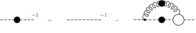
Figure 2.1: The ghost DSE AvS [01].

The gluon DSE is obtained in a similar manner as the ghost DSE, but in comparison to that, it is much more complex. Therefore, we only give a pictorial representation of the gluon DSE in Fig. 2.2. Please refer again to Ref. AvS [01] for an explicit expression.

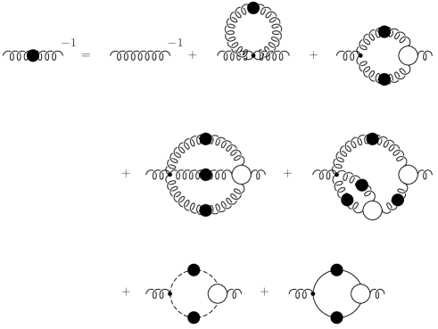
Figure 2.2: Diagrammatic representation of the gluon DSE. Adapted from Ref. AvS [01].

As in Fig. 2.1, wiggled lines refer to the gluon propagator in Fig. 2.2, whereas a line and a dashed line refer to the quark and ghost propagator, respectively. Lines carrying a full circle correspond to fully dressed propagators. Open circles denote full vertex functions.

For the DSE of the quark propagator a similar diagram as for the ghost DSE can be given. See Ref. AvS [01] for both an explicit and a pictorial representation.

2.2.1 Infrared behavior of ghost and gluon propagators in Landau gauge

If the full solution of QCD’s Dyson-Schwinger equations were available it would provide us with a solution to QCD. However, this has not been obtained so far. The main impediment is that the infinite tower of coupled nonlinear integral DSEs has to be truncated in order to be manageable. Thereby, the challenge is to use suitable truncations that respect as much as possible the symmetries of the theory. Doing so, solutions of the truncated systems might provide deep insights into many phenomena in hadron physics, because they may serve as input into bound state calculations based on the Bethe-Salpeter equations for mesons or the Faddeev equations for baryons.

Studying DSEs has become a subject of growing interest in recent years. See Refs. RW [94]; RS [00]; AvS [01]; MR [03] for a comprehensive overview. In particular, in Landau gauge or general covariant gauges considerable progress has been made in studying the low-momentum region for the coupled system of quark, gluon and ghost propagators. In contrast to earlier attempts Man [79]; ADJS [81]; AJS [82]; BP [89] where contributions of ghost fields were neglected, the more recent attempts, initiated by von Smekal et al. vSAH [97]; vSHA [98], have shown that the inclusion of ghost fields is important for the generation of a consistent infrared behavior of QCD Blo [01]. In fact, it has been shown in vSAH [97]; vSHA [98] that in the infrared momentum region a diverging ghost propagator is intimately related to a vanishing gluon propagator, both following a power law at low momentum.

We have given explicit expressions for the gluon and ghost propagators in Eq. (1.33) and (1.34), respectively. The corresponding renormalized dressing functions have been denoted by $Z$ and $J$. According to vSAH [97]; vSHA [98] these dressing functions are predicted to follow the power laws

$$Z(q^{2},\mu^{2}) \propto (q^{2}/\mu^{2})^{\kappa_{D}}$$ (2.5a)

$$J(q^{2},\mu^{2}) \propto (q^{2}/\mu^{2})^{-\kappa_{G}}\;$$ (2.5b)

in the limit $q^{2}\to 0$ with infrared exponents, $\kappa_{D}$ and $\kappa_{G}$, satisfying

$$\kappa_{D}=2\kappa_{G}\;.$$ (2.6)

This has been confirmed later by Atkinson and Bloch AB98b ; AB98a at the level in which the vertices in the DSEs are taken to be bare. Also investigations of the DSEs in flat Euclidean space-time performed by Fischer et al. FAR [02]; Fis [03]; FA [02] without angular approximations, as used in the former studies, support such an infrared behavior. The value of $\kappa_{G}$ depends on the truncation used, but in Landau gauge it has been argued that $\kappa_{G}\approx 0.595$ should be expected LvS [02]; Zwa [02]. Thus the ghost propagator is supposed to diverge stronger than $1/q^{2}$ and the gluon propagator to be vanishing in the infrared regime.

These findings are, as we shall see in Sec. 2.3.1 and 2.3.2, in agreement with the Kugo-Ojima confinement criterion KO [79] as well as with the Zwanziger-Gribov horizon condition Zwa [04, 94]; Gri [78]. According to the latter condition, a diverging ghost and a vanishing gluon propagator result from restricting the gluon fields to the Gribov region $\Omega$ Zwa [04].

Note, however, that quite recently Fischer et al. have investigated DSEs on a torus. They have found quantitative differences with the infinite volume results at small momenta FGA [06]; FP [06]. Moreover, Bloch has developed truncation schemes for the DSEs of the ghost, gluon and quark propagators Blo [01, 02] which preserve multiplicative renormalizability, in contrast to those schemes used in the references cited above. Furthermore, Bloch has demonstrated that a definite conclusion about the existence of infrared power-behaved gluon and ghost propagators cannot be reached yet.

We shall show in Sec. 4.3 that our lattice data and also those by others do not confirm Eq. (2.6), at least for the lattice momenta available at present. The values of the infrared exponents have been found to be different. Therefore, we think it is still an open question whether the infrared behavior as favored by current DSE studies is realized for lattice QCD in Landau gauge. However, if it is realized then it has interesting consequences for the running coupling constant discussed next.

2.2.2 A nonperturbative running coupling constant

From the renormalization of the ghost-gluon vertex, the renormalized coupling constant at the renormalization point $\mu$ is defined by

$$\alpha_{s}(\mu^{2})=\alpha(\Lambda^{2})\,\frac{Z_{3}(\Lambda^{2},\mu^{2})\widetilde{Z}^{2}_{3}(\Lambda^{2},\mu^{2})}{\widetilde{Z}^{2}_{1}(\Lambda^{2},\mu^{2})}\;.$$ (2.7)

Here $\alpha(\Lambda^{2})\mathrel{\mathop{\mathchar 58\relax}}=\textsl{g}_{0}^{2}(\Lambda^{2})/4\pi$ denotes the bare coupling constant that depends on the ultraviolet cutoff $\Lambda$ and the multiplicative constants, $Z_{3}$, $\widetilde{Z}_{3}$ and $\widetilde{Z}_{1}$, refer to the renormalization constants of the gluon and ghost propagators and of the ghost-gluon vertex, respectively. Long time ago, it has been shown by Taylor Tay [71] that to any order in perturbation theory the ghost-gluon vertex in Landau gauge is finite (see Sec. 2.2.3 for some discussions). Therefore, one may chose

$$\widetilde{Z}_{1}(\Lambda^{2},\mu^{2})=1.$$ (2.8)

Based on this and by using the relation between the bare and renormalized ghost and gluon dressing functions

$$J(q^{2},\mu^{2}) = \widetilde{Z}^{-1}_{3}(\Lambda^{2},\mu^{2})\;J_{B}(\Lambda^{2},q^{2})$$ (2.9a)

$$Z(q^{2},\mu^{2}) = Z^{-1}_{3}(\Lambda^{2},\mu^{2})\;Z_{B}(\Lambda^{2},q^{2})$$ (2.9b)

where $J(\mu^{2},\mu^{2})=Z(\mu^{2},\mu^{2})=1$, one can show that the product vSAH [97]; vSHA [98]

$$\alpha_{s}(q^{2})\mathrel{\mathop{\mathchar 58\relax}}=\alpha_{s}(\mu^{2})Z(q^{2},\mu^{2})J^{2}(q^{2},\mu^{2}),$$ (2.10)

is renormalization group invariant and defines a running coupling constant within the context of DSEs AvS [01]; AFLE [05]. In fact, with Eq. (2.7), (2.8) and (2.9) it holds that

$$\alpha_{s}(\mu^{2})Z(q^{2},\mu^{2})J^{2}(q^{2},\mu^{2})=\alpha(\Lambda^{2})Z_{B}(\Lambda^{2},q^{2})J^{2}_{B}(\Lambda^{2},q^{2}).$$

Obviously, the right hand side does not depend on the renormalization point $\mu^{2}$ and thus the combination of (renormalized) ghost and gluon dressing functions on the left hand side is renormalization-group-invariant. Evaluating the left hand side once at an arbitrarily chosen $\mu^{2}$ and once at $\mu^{2}=q^{2}$ one obtains the product given in Eq. (2.10) AFLE [05].

The definition of a running coupling constant by Eq. (2.10) has been first derived in vSAH [97]; vSHA [98]. Later it has been shown by Bloch Blo [01, 02] that after a reformulation of the DSEs for the ghost, gluon and quark propagators this coupling constant enters directly the kernel of the DSEs.

Assuming multiplicative renormalizability to hold beyond perturbation theory, and assuming also the power laws (Eq. (2.5)) for the dressing function being realized at infrared momenta according to the relation (2.6), then $\alpha_{s}(q^{2})$ has a finite infrared fixed point vSAH [97]; vSHA [98]. The precise value of $\alpha_{s}(0)$ depends on $\kappa_{G}$, but under certain assumption it has been shown to be LvS [02]

$$\alpha_{s}(0)\approx 8.915/N_{c}\qquad\textrm{for}\ SU(N_{c}).$$

However, we would like to stress already here that our lattice data for $\alpha_{s}(q^{2}>0)$ do not indicate the existence of a finite value at zero momenta (see Sec. 4.4.1). We have also found no indications for deviations from $\widetilde{Z}_{1}$ being constant (Sec. 4.4.2). Our lattice data presented in this thesis are in agreement with other lattice studies and, most notably, also agree qualitatively with recent investigation of DSEs on a torus FGA [06]; FP [06]. This, once more, puts the proposed form for infrared power laws into question.

2.2.3 The finiteness of the ghost-gluon vertex

Arguments were given first by Taylor Tay [71] that in Landau gauge the renormalization constant of the ghost-gluon vertex $\widetilde{Z}_{1}=1$. He showed that in this gauge the ghost-gluon vertex is finite in the ultraviolet momentum region and stays bare for a vanishing incoming ghost momentum. To motivate this we recall arguments given in Refs. MP [78]; AFLE [05] using the DSE for the full ghost-gluon vertex. A pictorial representation of this DSE is shown in Fig. 2.3.

Considering this figure, the argument goes at follows MP [78]; AFLE [05]: The bare ghost-gluon vertex in the interaction diagram (rightmost diagram) is proportional to the internal loop momentum $l_{\mu}$. Since in Landau gauge the gluon propagator $D_{\mu\nu}(l-q)$ is transverse, it holds that $l_{\mu}D_{\mu\nu}(l-q)=q_{\mu}D_{\mu\nu}(l-q)$ and thus the interaction diagram vanishes in the limit $q_{\mu}\rightarrow 0$ AFLE [05]. This implies (see Fig. 2.3)

$$T^{abc}_{\lambda\mu}(k,q)=g_{\lambda\mu}(A^{abc}q^{2}+B^{abc}k^{2}+C^{abc}r^{2})+D^{abc}k_{\lambda}k_{\mu}+\textrm{etc.}$$

as $k^{2}$, $r^{2}$ and $q^{2}\rightarrow 0$ so that $r^{\lambda}T^{abc}_{\lambda\mu}(k,q)$ vanishes MP [78]. Therefore, the full vertex equals the bare vertex at the subtraction point $p^{2}=k^{2}=r^{2}=0$ and there is no renormalization. This, however, is not true if one renormalizes at another point $\mu^{2}>0$, even though it remains true to lowest order in perturbation theory MP [78]. Note also that this argument would be invalidated if the two-ghost–two-gluon scattering kernel $T^{abc}_{\lambda\mu}(k,q)$ had an infrared divergence AFLE [05].

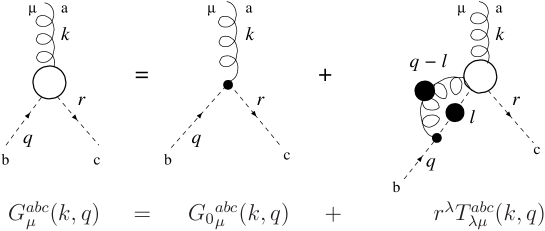
Figure 2.3: The Dyson-Schwinger equation of the ghost-gluon vertex.

We shall show in Sec. 4.4.2 that our lattice results for the renormalization constant $\widetilde{Z}_{1}$ do not support the existence of such a divergence in the particular MOM scheme $p^{2}=r^{2}$ and $k^{2}=0$. This was also seen by others CMM [04] in a similar lattice study of quenched $SU(2)$ gauge theory. Furthermore, semiperturbative calculations of $\widetilde{Z}_{1}$ using either $p^{2}=r^{2}=k^{2}=\mu^{2}$ or $p^{2}=r^{2};k^{2}=0$ show that such a divergence is absent. The analytical study presented in AFLE [05] also shows that the dressing of the ghost-gluon vertex remains finite if all external momenta vanish.

We also refer to the recent study B⁺05b where arguments in favor of a singular infrared behavior of the ghost-gluon vertex function is given.

2.3 Criteria for confinement in linear covariant gauges

Despite the success of QCD in describing strong interaction processes at high energies, there is still the unsolved and theoretically demanding problem what kind of mechanism confines QCD degrees of freedom, the quark and gluon states, and keeps them from being observed in the physical particle spectrum. In contrast to QED, where a one-to-one correspondence between basic fields and stable particles can be assumed, in QCD it cannot. Only hadronic amplitudes are physical and only color singlets can contribute to the physical state space of QCD.

For QCD in covariant gauges there is the additional subtlety that it requires a state space with indefinite metric. In order to allow for a quantum mechanical interpretation there has to be some mechanism which generates a subspace of (colorless) physical states that has a positive semi-definite metric.

In the following three criteria for confinement are briefly introduced, namely the Kugo–Ojima confinement scenario, the Gribov–Zwanziger horizon condition and the violation of reflection positivity of propagators corresponding to confined particles. These criteria are proposed to be sufficient to indicate confinement; and we will see in succeeding chapters that our lattice simulations show evidence for those criteria to be satisfied in lattice QCD in Landau gauge.

2.3.1 The Kugo–Ojima confinement scenario

In this section we temporarily switch from the functional formalism to the covariant operator formalism which is more suitable in the present context. This formalism takes fields as operators, rather than as c-numbers, and they satisfy (anti-) commutation relations. Also the notion of BRST symmetry is important for a formulation of a covariant operator formalism. For a comprehensive account of this subject we refer to the book NO [90] by Nakanishi and Ojima where most of the material summarized below is exhaustively discussed.

Requirements for a physical S-matrix to exist

Covariant quantum gauge theories require state spaces $\mathcal{V}$ with indefinite metric. If one can show, however, that (a) the Hamiltonian operator of a theory is hermitian so that a $S$-matrix $S$ exists in $\mathcal{V}$ satisfying $\langle S\Psi_{1}|S\Psi_{2}\rangle=\langle\Psi_{1}|\Psi_{2}\rangle$ and (b) there is a subspace $\mathcal{V}_{\textrm{phys}}\subseteq\mathcal{V}$ which not only is invariant under time evolution, but also (c) has a positive semi-definite inner product $\langle\cdot|\cdot\rangle$, then a physical $S$-matrix $S_{\textrm{phys}}$ can be defined in the completed quotient space

$$\mathcal{H}_{\textrm{phys}}\equiv\overline{\mathcal{V}_{\textrm{phys}}/\mathcal{V}_{0}}\;.$$

$\mathcal{H}_{\textrm{phys}}$ denotes a Hilbert space with positive definite inner product, and $S_{\textrm{phys}}$ is unitary with respect to this Hilbert space structure. The subspace $\mathcal{V}_{0}\subset\mathcal{V}_{\textrm{phys}}$ contains the zero-norm states of the positive semi-definite subspace $\mathcal{V}_{\textrm{phys}}$ and is orthogonal to it, i.e. $\mathcal{V}_{0}\perp\mathcal{V}_{\textrm{phys}}$ [NO, 90, A.2].

It can be shown that the first two requirements, (a) and (b), are satisfied automatically for QCD in covariant gauges if the Lagrangian density $\mathcal{L}_{\textrm{eff}}^{r}$ (Eq. (1.27)) is hermitian and the physical subspace $\mathcal{V}_{\textrm{phys}}$ is defined as the kernel of the BRST–charge $Q_{B}$, i.e.

$$\mathcal{V}_{\textrm{phys}}=\ker Q_{B}\equiv\{\Psi\in\mathcal{V}\mathrel{\mathop{\mathchar 58\relax}}Q_{B}\Psi=0\}$$ (2.11)

where $Q_{B}$ is assumed to be an unbroken generator of BRST symmetry.

The proof of condition (c), the positive semi-definiteness of the inner product in $\mathcal{V}_{\textrm{phys}}$, however, is a nontrivial problem and requires a detailed analysis of the inner product structure of both the total state space $\mathcal{V}$ and the physical subspace $\mathcal{V}_{\textrm{phys}}$ NO [90].

Representations of the BRST algebra

Such an analysis has been done by Kugo and Ojima KO [79] long ago from the viewpoint of the BRST–algebra given by

$$\left\{Q_{B},Q_{B}\right\} = 0,\qquad\left[iQ_{c},Q_{B}\right]=Q_{B},\qquad\left[Q_{c},Q_{c}\right]=0.$$

Here $Q_{c}$ denotes the FP–ghost charge which is assumed to be unbroken as it is assumed for $Q_{B}$.

The BRST–algebra has two types of irreducible representations, namely singlet and doublet representations. While a doublet consists of a so-called parent state $|\pi\rangle$ and a daughter state $|\delta\rangle\equiv Q_{B}|\pi\rangle\neq 0$ (i.e. the BRST transform of $|\pi\rangle$), a BRST–singlet is a state that is annihilated by $Q_{B}$ without having a corresponding parent state in $\mathcal{V}$.

Kugo and Ojima have shown that to each BRST–doublet there exists always another being FP-conjugate to it, i.e. with opposite eigenvalues of $iQ_{c}$. This FP-conjugate pair of BRST–doublets is called a BRST–quartet. Any state in $\mathcal{V}$ can be classified to be either a BRST–singlet or to belong to a BRST–quartet and it can be shown that this exhausts all possible representations of the BRST–algebra in spaces with indefinite inner product. We will see below that this classification is important, in that under certain conditions, colorless asymptotic states are BRST–singlets which then can be identified with physical particle states. On the other hand colored asymptotic states are members of a BRST–quartet and, therefore, do not appear in $S$-matrix elements.

To see this note first that daughter states $|\delta\rangle$ and BRST–singlet states (with no parents) belong to the physical space $\mathcal{V}_{\textrm{phys}}$ as defined in Eq. (2.11). However, daughter states are orthogonal to all states $\Psi\in\mathcal{V}_{\textrm{phys}}$

$$\langle\Psi|\delta\rangle=\langle\Psi|Q_{B}|\pi\rangle=0$$

and so cannot contribute to any element of the physical $S$-matrix $S_{\textrm{phys}}$. All the physical content is contained in the physical Hilbert space

$$\mathcal{H}_{\textrm{phys}}\equiv\overline{\mathcal{V}_{\textrm{phys}}/\mathcal{V}_{0}}\simeq\mathcal{V}_{s}.$$ (2.12)

which is isomorphic to the space $\mathcal{V}_{s}$ of BRST–singlet states. Here

$$\mathcal{V}_{0}=\operatorname{im}Q_{B}=\{|\delta\rangle\in\mathcal{V}\mathrel{\mathop{\mathchar 58\relax}}|\delta\rangle=Q_{B}|\pi\rangle,|\pi\rangle\in\mathcal{V}\}$$

is the set of all zero-norm (daughter) states.

Confinement of colored asymptotic fields

Under the assumption of $Q_{B}$ and $Q_{c}$ to be unbroken, the classification of representations of the BRST–algebra can be translated into the properties of creation and annihilation operators of asymptotic fields. Intuitively, these are understood to create asymptotic particle states which are observable in scattering experiments long before and long after collisions.

Asymptotic states constitute two Fock spaces, $\mathcal{V}_{\textrm{in}}$ and $\mathcal{V}_{\textrm{out}}$. By the postulate of asymptotic completeness they are equal to the whole Hilbert space $\mathcal{V}$, i.e.

$$\mathcal{V}_{\textrm{in}}=\mathcal{V}=\mathcal{V}_{\textrm{out}}.$$

This is an important postulate and in particular it guarantees that any operator is expressible in terms of asymptotic fields NO [90]. For any two states $|f\rangle,|g\rangle\in\mathcal{V}$ an asymptotic field $\phi^{\textrm{as}}$ is defined as the weak limit

$$\lim_{x^{0}\rightarrow\mp\infty}\;\langle f|\phi^{(r)}(x)-\phi^{\textrm{as}}(x)|g\rangle=0$$

of the corresponding renormalized operator $\phi^{(r)}=Z^{-1/2}\phi$.

Due to confinement there must be some mechanism that causes colored asymptotic fields, if any, not to contribute to any physical $S$-matrix element. Such a mechanism, the quartet mechanism, has been proposed by Kugo and Ojima KO [79] for covariant gauge theories.

They have analyzed the total state space $\mathcal{V}$ as the Fock space of asymptotic fields and showed that any asymptotic field is either a BRST–singlet or a quartet member, because no other irreducible representation exists as they have shown (see above). If combined with the fact that under certain conditions (specified below) the charge $Q^{a}$ of global gauge transformation is BRST–exact and can be written as (see next subsection)

$$Q^{a}=\left\{Q_{B},\mathcal{C}\right\}\qquad\textrm{where}\quad\mathcal{C}\mathrel{\mathop{\mathchar 58\relax}}=\int d^{3}x(D_{0}\bar{c})^{a}(x).$$ (2.13)

then for any physical states $|\Psi_{1}\rangle,|\Psi_{2}\rangle\in\mathcal{V}_{\textrm{phys}}$ it holds that

$$\langle\Psi_{1}|Q^{a}|\Psi_{2}\rangle=0.$$

The charge $Q^{a}$ vanishes in the physical Hilbert space $\mathcal{H}_{\textrm{phys}}$ defined in Eq. (2.12). Consequently, if there were colored asymptotic fields, they would belong to the BRST–quartet representations. BRST–singlets, on the other hand, are necessarily colorless and thus can be identified with physical particles. This is known as confinement by the quartet mechanism.

One example is the so called elementary quartet that can be easily deduced from the BRST transformation of $A_{\mu}$ and $\bar{c}^{a}$ (Eq. (1.25) or (1.31)). Obviously, it consists of the parent states $|A^{a}_{\mu}\rangle$ and $|\bar{c}^{a}\rangle$ and of the daughter states $|D^{ab}_{\mu}c^{b}\rangle$ and $|B^{a}\rangle$. As shown in Kug [95] the corresponding (massless) asymptotic states — they describe longitudinally polarized gluons, ghost and antighosts — also form a BRST–quartet representation and are therefore not observable in the physical spectrum.

It is also expected that the quartet mechanism applies to transverse gluon and quark states, as far as they exist asymptotically. A violation of (reflection) positivity (see Sec. 2.3.3) for such states entails these are not observable either NO [90]; AvS [01]. In Sec. 5.3 it is shown that the lattice gluon propagator in Landau gauge violates reflection positivity explicitly which thus supports this expectation.

The Kugo-Ojima confinement criteria

Color confinement by the quartet mechanism can only take place if there is an unbroken and BRST–exact color charge $Q^{a}$.

In general, $Q^{a}$ is a generator of the global gauge symmetry that, in addition to the BRST symmetry, is left in the gauge-fixed effective Lagrangian density $\mathcal{L}_{\textrm{eff}}$. The corresponding symmetry transformations are given in Eq. (1.7) if there the parameters $\omega^{a}$ are taken to be space-time independent parameters. Being a global symmetry there exist Noether currents $J^{a}_{\mu}$ which are conserved , i.e.

$$\partial_{\mu}J^{a}_{\mu}=0\,.$$ (2.14)

As pointed out first by Ojima Oji [78], these currents enter the equation of motion for the gauge fields in the form

$$gJ^{a}_{\mu}+\partial_{\nu}F^{a}_{\nu\mu}=\{Q_{B},D_{\mu}\bar{c}^{a}\}.$$ (2.15)

This equation is usually referred to as the quantum Maxwell equation in the non-abelian case, because for any physical states $|\psi_{1}\rangle,|\psi_{2}\rangle\in\mathcal{V}_{\textrm{phys}}$ the classical Maxwell-type equation $\langle\psi_{1}|(\partial_{\nu}F_{\nu\mu}^{a}+gJ^{a}_{\mu})|\psi_{2}\rangle=0$ holds.

Since the conservation law in Eq. (2.14) allows adding arbitrary terms of the form $\partial_{\mu}f^{a}_{[\mu\nu]}$ to $J^{a}_{\mu}$ with $f^{a}_{[\mu\nu]}$ being a local antisymmetric tensor, one could be tempted to define the global charge operators $Q^{a}$ as the spatial integral of the current

$$J^{{}^{\prime}a}_{\mu}=J^{a}_{\mu}+\frac{1}{g}\partial_{\nu}F^{a}_{\nu\mu}$$

such that the BRST–exact expression in Eq. (2.13) is retrieved. But this naive definition of $Q^{a}$ is ill-defined due to massless one-particle contributions to $J^{a}_{\mu}(x)$, $\partial_{\nu}F^{a}_{\mu\nu}$ and $\{Q_{B},D_{\mu}\bar{c}^{a}\}$ which cause the integral to not converge Kug [95].

If however these contributions are consistently incorporated in the definition of $Q^{a}$, a well-defined expression is obtained (see Kug [95] for details). This is important, since with the Goldstone theorem this automatically implies that condition (B) formulated in the original work KO [79] of Kugo and Ojima, namely

(B)  $Q^{a}$ is not spontaneously broken,

is satisfied in the indefinite metric space $\mathcal{V}$. If furthermore a certain parameter $\textsf{u}^{ab}$, the Kugo-Ojima confinement parameter, turns out to satisfy condition

(A)  $\textsf{u}^{ab}=-\delta^{ab}$,

then the color charge $Q^{a}$ takes the BRST–exact form as given in Eq. (2.13) and color confinement by the quartet mechanism

$$\langle\Psi_{1}|Q^{a}|\Psi_{2}\rangle=0\qquad\Psi_{1},\Psi_{2}\in\mathcal{V}_{\textrm{phys}}$$

takes place. But this holds only if condition (A) is fulfilled. Otherwise we cannot identify BRST–singlet states in the physical Hilbert space $\mathcal{H}_{\textrm{phys}}$ with color singlets.

To investigate whether condition (A) is realized, the Kugo-Ojima confinement parameter $\textsf{u}^{ab}$ can be obtained as the zero–momentum limit

$$\textsf{u}^{ab}\mathrel{\mathop{\mathchar 58\relax}}=\lim_{p^{2}\rightarrow 0}u^{ab}(p^{2})$$ (2.16)

of a function $u^{ab}(p^{2})$ which itself may be defined through the correlation function (see, for instance, Kug [95] or AvS [01])

$$\int d^{4}xe^{ip(x-y)}\left\langle D^{ae}_{\mu}c^{e}(x)\textsl{g}_{0}f^{bcd}A^{d}_{\nu}(y)\bar{c}^{c}(y)\right\rangle=\mathrel{\mathop{\mathchar 58\relax}}\left(\delta^{\mu\nu}-\frac{p_{\mu}p_{\nu}}{p^{2}}\right)u^{ab}(p^{2}).$$ (2.17)

To our knowledge a direct determination of $\textsf{u}^{ab}$ in terms of a lattice calculation of $u^{ab}(p^{2})$ has never been done. There are a few explorative lattice studies NF00b ; NF00a ; FN04a ; FN04b , but these are based on data of the ghost renormalization function $\widetilde{Z}_{3}$ (see below for the relation between $\widetilde{Z}_{3}$ and u.). The major problem is that in a lattice simulation $u^{ab}(p^{2})$ can be calculated only at finite momenta $p$ and the data then have to be extrapolated to $p=0$ for which a suitable ansatz has to be chosen.

The ghost propagator in the infrared is related to $\boldsymbol{u(p)}$

In Landau gauge the calculation of the correlation function in Eq. (2.17) can be even circumvented, because it has been shown Kug [95] that in this gauge the ghost dressing function $J$ is related to $u^{ab}(p^{2})\mathrel{\mathop{\mathchar 58\relax}}=\delta^{ab}u(p^{2})$ according to

$$J(p^{2})=\frac{1}{1+u(p^{2})+p^{2}v(p^{2})}$$ (2.18)

and $v(p^{2})$ is an arbitrary function (see Kug [95] for a definition). In the zero-momentum limit this yields

$$J(0)=\frac{1}{1+u(0)}\;.$$ (2.19)

Therefore, if condition (A) is realized in QCD then the ghost dressing function in Landau gauge should diverge for vanishing momenta. Turning the argument around, if the ghost propagator is found to be more singular than a simple pole this may serve as a sufficient criterion for the Kugo-Ojima confinement scenario to be realized.

Based on this arguments the infrared behavior of the ghost propagator as extracted from the corresponding truncated systems of DSE, has been stated to realize the Kugo-Ojima confinement scenario for QCD in Landau gauge. In support of this, in Sec. 4.3 we will show that also the ghost propagator as calculated in lattice simulations diverges stronger than a simple pole, albeit with different exponent compared to the one found in DSE studies.

More importantly, however, in Sec. 5.2 we present data for the Kugo-Ojima confinement parameter $u^{ab}(p)$ at finite momentum $p$ and compare these data to those of the ghost propagator. The data indicate $u^{ab}(p)$ to become proportional to $-\delta^{ab}$ in the limit of vanishing momenta. So the Kugo–Ojima confinement scenario seems to be realized for QCD in Landau gauge.

2.3.2 The Gribov–Zwanziger horizon condition

In the previous section we have seen that the infrared behavior of the ghost propagator is intimately connected to one condition of the Kugo–Ojima confinement criteria. In fact, if condition (A) is fullfilled then the ghost dressing function must be infrared divergent.

In coincidence with this, there is another condition, namely the Gribov–Zwanziger horizon condition Gri [78]; Zwa [93], that also requires the ghost dressing function to diverge at vanishing momentum. In fact, the horizon condition states that the ghost propagator $G$ in Landau gauge diverges stronger than $1/p^{2}$ in the zero-momentum limit, i.e. Zwa [02]

$$\lim_{p^{2}\rightarrow 0}\left[p^{2}G(p)\right]^{-1}=0.$$ (2.20)

Basically, this limit is a consequence of the expectation that the infrared modes of the gauge fields are very close to the Gribov horizon $\partial\Omega$ and hence give rise to an accumulation of small non-zero eigenvalues of the FP operator Zwa [94, 93]; Zwa91b . Since the ghost propagator, essentially, is the inverse of this operator, it must diverge in the infrared.

Remarkably, the horizon condition as given in Eq. (2.20) allows us to renormalize the ghost propagator at $p=0$ in the form of a nonperturbative formula for the corresponding renormalization constant $\widetilde{Z}_{3}$ (see Zwa [04] for details). This formula disagrees with the usual perturbative expression for $\widetilde{Z}_{3}$, but it satisfies the perturbative renormalization-group flow equation. If used together with the DSE for the ghost propagator it even yields an infrared anomalous dimension $\kappa_{G}$ for it, such that it behaves like Zwa [04]

$$G(p)\sim\frac{1}{p^{2}}\left(\frac{\mu^{2}}{p^{2}}\right)^{\kappa_{G}}$$

in the infrared. This is in agreement with the infrared behavior of the ghost and gluon propagators extracted from their Dyson-Schwinger equations vSAH [97]; AvS [01]; LvS [02].

Furthermore, it has been argued by Zwanziger Zwa91b ; Zwa [92] that the gluon propagator in Landau gauge vanishes in the infrared, i.e.

$$\lim_{p^{2}\rightarrow 0}D(p)=0,$$

because the infrared components $A(k)$ of the gluon field are suppressed by the proximity of the Gribov horizon in infrared directions Zwa [02].

In our study we will not only check for the infrared limits of both the gluon and ghost propagators as given above, but we will also show that the accumulation of near-to-zero eigenvalues of the FP operator increases with enlarging the physical volume (see Sec. 5.1, Sec. 5.2 and Sec. 6.2). Therefore, gauge configurations at the Gribov horizon seem to dominate the infrared properties of lattice Landau gauge theory in the thermodynamic limit.

2.3.3 Violation of reflection positivity as a criterion for confinement

The mechanism for confinement by Kugo and Ojima introduced in Sec. 2.3.1 relies on the existence of an unbroken BRST symmetry beyond perturbation theory. This, however, has not been proven yet and thus the Kugo-Ojima scenario should not necessarily apply to QCD. Nevertheless, the numerical results that we will discuss in Sec. 5.2, but also recent studies of truncated systems of Dyson-Schwinger equations for the ghost and gluon propagators (see next section) favor the Kugo-Ojima confinement scenario to be realized for QCD in Landau gauge.

In any case, there is another particular criterion for confinement that has been proposed in recent years (see e.g. AvS [01]; ADFM [04]) and is focused on in this study too, namely the violation of reflection positivity. In fact, reflection positivity is an essential part of the famous Osterwalder-Schrader axioms OS [73, 75] for Euclidean quantum field theory. Arbitrary partial sums of Euclidean $n$-point functions have to fulfill those axioms to ensure their analytic continuation to the physically interesting functions in Minkowski space. They thus guarantee the reconstruction of a Gårding-Wightman relativistic quantum field theory. This is important in order to arrive at a physical interpretation.

For the purpose of our study there is no need to go into detail about all the Osterwalder-Schrader axioms. We will rather focus on the notion of reflection positivity which states that an Euclidean Green’s function (Schwinger function) $\Delta$ has to satisfy

$$\sum_{n,m}\int \left[\prod_{i=1}^{n}d^{4}x_{i}\right]\left[\prod_{j=1}^{n}d^{4}y_{j}\right]\;f^{*}(\Theta x_{1},\ldots,\Theta x_{n})$$

$$\cdot\Delta(\Theta x_{1},\ldots,\Theta x_{n},y_{1},\ldots,y_{n})f(y_{1},\ldots,y_{n})\;\geq\;0.$$ (2.21)

Here $f$ refers to a complex valued test function with support for positive (Euclidean) times, i.e. $f(x_{1},\ldots,x_{n})=0$ for any $x^{4}_{i}<0$; and $\Theta$ is the reflection operator that acts on $x_{i}$ according to: $\Theta x_{i}=(\textbf{x}_{i},-x^{4}_{i})$.

In particular for a generic (Euclidean) 2-point function $\Delta(x,y)=\Delta(x-y)$, reflection positivity is a necessary and sufficient condition (see AvS [01]) for the existence of a Källen-Lehmann representation Käl [52]; Leh [54]. This is a spectral representation of 2-point functions with positive, but generally unknown, spectral density $\rho(m^{2})$ which in momentum space takes the form AvS [01]; A⁺ [97]; CMT [05]

$$\Delta(p)=\int_{0}^{\infty}dm^{2}\;\frac{\rho(m^{2})}{p^{2}+m^{2}}\qquad\textrm{with}\quad\rho(m^{2})\geq 0.$$ (2.22)

The absence of a Källen-Lehmann representation for a particular 2-point function is a sufficient condition for confinement of the corresponding particle, because then it cannot be interpreted in terms of stable particle states.

Considering the temporal correlator $C(t,\textbf{p}^{2})$, the absence of such a representation can be even formulated more straightforward. In fact, $C(t,\textbf{p}^{2})$ is the Fourier transform of Eq. (2.22) and takes the form AvS [01]

$$C(t,\textbf{p}^{2})=\frac{1}{\pi}\int^{\infty}_{0}\!\!dp_{4}\cos(p_{4}t)\int_{0}^{\infty}\!\!dm^{2}\frac{\rho(m^{2})}{p_{4}^{2}+\omega^{2}}=\int^{\infty}_{0}\!\!dm^{2}\rho(m^{2})\frac{\pi}{2\omega}\,e^{-\omega t}$$

where $\omega^{2}=m^{2}+\textbf{p}^{2}$. After substitution this gives

$$C(t,\textbf{p}^{2})=\int_{\sqrt{\textbf{p}^{2}}}^{\infty}d\omega\;\rho(\omega^{2}-\textbf{p}^{2})\,e^{-\omega t}.$$ (2.23)

One clearly sees that if the spectral density $\rho$ is a positive function then the temporal correlator $C(t,\textbf{p}^{2})$ is positive as well, but it does not hold in general the other way. If on the contrary $C(t,\textbf{p}^{2})$ is found to be negative for a certain range in $t$, i.e.

$$C(t,\textbf{p}^{2})<0$$ (2.24)

there cannot be a positive spectral density and thus reflection positivity is violated. This is an indication for confinement AvS [01]; CMT [05].

For the gluon two-point function reflection-positivity violation, of course, is expected to happen. However, it has never be shown explicitly in lattice simulations for the case of $SU(3)$. In three-dimensional pure $SU(2)$ gauge theory numerical evidence for reflection-positivity violation of the lattice Landau gluon propagators has been given CMT [05]. This study shows that also the $SU(3)$ gluon propagator in Landau gauge violates reflection positivity for the quenched and unquenched case.

We note in passing, that if the gluon propagator $D(p)$ in momentum space would be infrared vanishing, as expected from the proximity of the Gribov horizon (see the previous section), then it would violate reflection positivity maximally. This can be seen from

$$0=D(p=0)=\int d^{4}x\,D(x).$$

This can only happen if the gluon propagator in coordinate space, $D(x)$, contains positive as well as negative contributions of equal integrated strength ADFM [04].

The ghost propagator violates reflection positivity trivially which can be deduced already from its bare expression. Hence ghosts are explicitly unphysical indeed. The unphysical spin–statistic relation of ghost fields already suggests this.

Chapter 3 QCD Green’s functions in lattice Landau gauge

[0,l,T,] his chapter very briefly introduces the lattice regularization of QCD. We concentrate on the Wilson formulation of QCD with and without clover improved Wilson fermions as employed for this study. After specifying some general aspects we focus on lattice QCD in Landau gauge and define all relevant gauge-variant observables which are analyzed in the following chapters.

3.1 Basics of lattice QCD

We know that the very definition of a quantum field theory, as QCD, requires a regularization which often breaks some of the underlying symmetries of the classical theory and introduces a new scale into the theory Has [98]. At present the only known regularization of QCD beyond perturbation theory is the lattice regularization which discretizes Euclidean space-time into a lattice of points. Thereby, the lattice spacing $a$ serves as a regulator of the theory that renders all ultraviolet divergences, usually encountered in QCD, finite. Unlike field theory with a naive ultraviolet cutoff, the lattice formulation maintains exact gauge invariance Mut [98]; BHL⁺ [05]. Furthermore, the lattice regularization offers the possibility to investigate nonperturbative aspects of QCD in terms of numerical Monte Carlo (MC) simulations. Therefore, it is a valuable tool for cross-checking results obtained using other nonperturbative methods, for example the DS approach to QCD.

It is beyond the scope of this thesis to adequately describe all aspects of lattice QCD. Therefore, we shall recall only some basic points important for the following. For a comprehensive introduction on the subject we refer to standard textbooks Cre [83]; MM [94]; Rot [97]; Smi [02] as well as to the lectures Kog [83]; Lep [00]; Gup [97]; Dav [02]; Lüs [03]; Dav [05], to name but a few. Most of the material summarized below can be found there. To find out about the most recent developments in the field the proceedings AHI⁺ [04]; B⁺05a ; IMM [05] of the yearly Lattice Conferences provide a good starting point.

3.1.1 The lattice and its fields

Very briefly, lattice QCD is a discretization of QCD in Euclidean space. It replaces the four-dimensional space-time continuum through a hypercubic lattice and restricts fermion and antifermion fields, $\psi_{x}$ and $\bar{\psi}_{x}$ respectively, to dwell on the lattice sites $x$. Rather than specifying the gauge fields by gluon fields $A_{\mu}(x)$, on the lattice gauge fields are associated with links joining adjacent lattice sites, $x$ and $x+\hat{\mu}$. Here and in the following $\hat{\mu}$ is a unit vector in the $x_{\mu}$ direction of space-time. The lattice spacing $a$ is the distance between adjacent lattice sites. The gauge fields — also known as link variables or even just as links — are usually denoted by $U_{x,\mu}$ and take values in a compact Lie group, here $SU(3)$. They are the lattice version of the parallel transport matrix between adjacent sites and therefore are related to the continuum gluon fields $A_{\mu}(x)$ by the line integral (see e.g. LSWP [99])

$$U_{x,\mu}\equiv\textsf{P}\exp\left\{i\textsl{g}_{0}\int^{1}_{0}A_{\mu}(x+at\hat{\mu})\,dt\right\}\;\simeq\;e^{ia\textsl{g}_{0}A_{\mu}(x+\hat{\mu}/2)}+O\left(a^{3}\right).$$ (3.1)

Here P denotes path ordering of the gluon fields along the integration path such that gluon fields $A_{\mu}(x+at\hat{\mu})$ with larger $t$ stand to the left of those with smaller $t$. The gauge fields $U$ are taken in place of the gluon fields for the purpose of maintaining explicit gauge invariance on the finite lattice BHL⁺ [05]. A gauge invariant formulation of lattice QCD directly in terms of the gluon fields is not possible Lep [00].

Quantization of lattice QCD is done in the functional integral formalism, i.e. expectation values of different observables are given in terms of path integrals over the gauge and quark field variables MM [94]

$$\langle\mathcal{O}\rangle=\frac{1}{Z}\int[\mathcal{D}U,\mathcal{D}\bar{\psi},\mathcal{D}\psi]\,\mathcal{O}[\psi,\bar{\psi},U]\;e^{-S_{QCD}[U,\bar{\psi},\psi]}\;.$$ (3.2)

Here the partition function $Z$ is chosen such that $\langle\mathbb{1}\rangle$ = 1 and $\mathcal{O}[\psi,\bar{\psi},U]$ denotes an arbitrary function of the field variables, for instance, $n$ pairs of quark fields and a product of link variables

$$\mathcal{O}[\psi,\bar{\psi},U]=\psi^{a_{1}}_{x_{1}}\cdots\bar{\psi}^{b_{1}}_{y_{1}}\cdots U_{z_{1}\mu_{1}}\cdots\;.$$

For simplicity, the indices $a_{i}$ and $b_{i}$ denote the set of all internal symmetry indices, like color and spinor degrees of freedom. The color indices of link variables are hidden. Lattice sites are denoted by $x_{i}$, $y_{i}$ or $z_{i}$ and $\mu_{i}$ refers to one particular direction on the lattice.

In contrast to any formulation in the continuum, the lattice action $S_{QCD}$ maintains exact gauge invariance. Since the gauge fields take values only in the group $SU(3)$, i.e. they are restricted to a compact manifold, the functional integration measure is well-defined and gauge-fixing is not necessary if gauge-invariant observables $\mathcal{O}[\psi,\bar{\psi},U]$ are considered. However, in this thesis gauge-variant quantities are investigated, in particular in Landau gauge. Therefore, gauge-fixing becomes necessary here as well. In Sec. 3.2 this is discussed in more detail.

3.1.2 The Wilson action with clover-improved fermions

Apart from the requirement of local gauge invariance the definition of $S_{QCD}$ is not unique. There are infinite ways to define a lattice action of QCD, but any definition has to be such that it takes the classical continuum form for vanishing lattice spacing $a$. This freedom allows for a clever reduction of systematic errors caused by finite lattice spacings. Any reasonable formulation will give the same continuum theory up to finite renormalizations of the gauge coupling and the quark masses Lüs [03].

Common actions used in the literature consist of two parts, a gauge $S_{G}$ and a fermionic part $S_{F}$, i.e. they are of the general form

$$S_{QCD}=S_{G}[U]+S_{F}[U,\bar{\psi},\psi]\;.$$ (3.3)

Both parts depend on the gauge fields $U\equiv\{U_{x,\mu}\}$ and the fermionic part contains in addition bilinear expressions in the fermion fields $\bar{\psi}$ and $\psi$ constructed such that the whole action is manifestly gauge invariant.

For the gauge part we have employed the standard Wilson gauge action Wil [74] throughout this study. It is given by the sum

$$S_{G}[U]\mathrel{\mathop{\mathchar 58\relax}}=\beta\sum_{x}\sum_{1\leq\mu<\nu\leq 4}\left(1-\frac{1}{N_{c}}\operatorname{\mathfrak{Re}}\operatorname{Tr}\square_{x,\mu\nu}\right)$$ (3.4)

over traces of plaquettes denoted here by

$$\square_{x,\mu\nu}\mathrel{\mathop{\mathchar 58\relax}}=U_{x,\mu}U_{x+\hat{\mu},\nu}U^{\dagger}_{x+\hat{\nu},\mu}U^{\dagger}_{x,\nu}\;.$$ (3.5)

It represents a square of four links on the lattice. The parameter $\beta$ is defined such that $S_{G}$ takes its classical continuum form in the limit $a\rightarrow 0$, i.e. it is defined as

$$\beta\mathrel{\mathop{\mathchar 58\relax}}=\frac{2N_{c}}{\textsl{g}_{0}^{2}}$$ (3.6)

where $N_{c}=3$ for $SU(3)$ and $\textsl{g}_{0}$ is the bare coupling constant.

For the fermionic part $S_{F}$ there are various definitions in use which either belong to the family of Wilson or of Staggered fermion actions or start therefrom. For the purpose of this study fermions of the Wilson type have been employed. In fact, our choice are clover–improved Wilson fermions SW [85]; LSSW [96]. The corresponding part of the action can be written as

$$S_{F}[U,\bar{\psi},\psi]=a^{4}\sum_{f,x,y}\bar{\psi}^{f}_{x}\,Q_{xy}\,\psi^{f}_{y}$$ (3.7)

where for each flavor $f=1,\ldots,N_{f}$ the fermion matrix $Q$ is defined to act upon the (Grassmann valued) fermion fields, $\bar{\psi}_{x}$ and $\psi_{y}$, according to

$$\sum_{xy}\bar{\psi}_{x}Q_{xy}\psi_{y}\mathrel{\mathop{\mathchar 58\relax}}=\sum_{x}\Bigg{\{}\frac{1}{a}\bar{\psi}_{x}\psi_{x} -{\frac{\kappa}{a}}\sum_{\mu}\bar{\psi}_{x}\,U^{\dagger}_{x-\hat{\mu},\mu}\left[1+\gamma_{\mu}\right]\psi_{x-\hat{\mu}}$$

$$-\frac{\kappa}{a}\sum_{\mu}\bar{\psi}_{x}\,U_{x,\mu}\left[1-\gamma_{\mu}\right]\psi_{x+\hat{\mu}}$$

$$-\frac{\kappa a}{2}\,c_{sw}\,\textsl{g}_{0}\,\sum_{\mu\nu}\bar{\psi}_{x}\,\sigma_{\mu\nu}F_{x,\mu\nu}^{\textrm{clover}}\psi_{x}\Bigg{\}}$$ (3.8)

(see e.g. GHP⁺ [05]). The fermion fields are normalized such that they correspond to the continuum fields by rescaling $\psi\rightarrow 1/\sqrt{2\kappa}\,\psi$. Due to the last term in Eq. (3.8), $S_{F}$ is sufficient to remove all $O\left(a\right)$ errors for on-shell quantities. The value of the parameter $c_{sw}$ depends on $\textsl{g}_{0}$ and has to be tuned appropriately. The clover field-strength tensor is given by

$$F^{\textrm{clover}}_{x,\mu\nu}\mathrel{\mathop{\mathchar 58\relax}}=\frac{1}{8i\textsl{g}_{0}a^{2}}\sum_{\pm\mu,\pm\nu}\Big{(}\square_{x,\mu\nu}-\square^{\dagger}_{x,\mu\nu}\Big{)}\,,$$ (3.9)

where the definition of the plaquette (see Eq. (3.5)) has been extended such that the $\mu$, $\nu$ directions can be negative GHP⁺ [05]. The hopping parameter $\kappa$ is related to the (subtracted) bare quark mass via

$$m=\frac{1}{2a}\left(\frac{1}{\kappa}-\frac{1}{\kappa_{c}}\right)$$ (3.10)

where $\kappa_{c}$ is defined as the value of $\kappa$ at which the pion mass vanishes. In this study we consider only the cases of either infinite heavy quarks, i.e. no quarks ($N_{f}=0$) or $N_{f}=2$ mass degenerate quarks. The former case is known as the quenched approximation of QCD, whereas the latter is an approximation to the real, unquenched world of two light and a number of heavier quarks that do respond to the gauge field.

3.1.3 Vacuum expectation values from MC simulations

After having defined the lattice action we now come back to the definition of vacuum expectation values in Eq. (3.2) and outline the way Monte Carlo (MC) simulations are employed to calculate them. First note that the integral over the fermionic variables can be done instantly due to their Grassmann nature. We obtain MM [94]

$$\langle\mathcal{O}\rangle \equiv\left\langle\psi_{x_{1}}\bar{\psi}_{y_{1}}\cdots\psi_{x_{n}}\bar{\psi}_{y_{n}}\mathcal{G}[U]\right\rangle$$

$$=\frac{1}{Z}\int[\mathcal{D}U]\,e^{-S_{\textrm{eff}}[U]}\;\mathcal{G}[U]\sum_{z_{1},\ldots,z_{n}}\epsilon^{z_{1},\ldots,z_{n}}_{x_{1},\ldots,x_{n}}\;Q^{-1}_{z_{1},y_{1}}[U]\cdots Q^{-1}_{z_{n},y_{n}}[U]$$ (3.11)

where the effective action $S_{\textrm{eff}}[U]$ (see Eq. (3.12)) depends only on gauge fields. $\mathcal{G}[U]$ denotes an arbitrary function depending on link variables only. The tensor $\epsilon^{z_{1},\ldots,z_{n}}_{x_{1},\ldots,x_{n}}\mathrel{\mathop{\mathchar 58\relax}}=1$ ($\epsilon^{z_{1},\ldots,z_{n}}_{x_{1},\ldots,x_{n}}\mathrel{\mathop{\mathchar 58\relax}}=-1$) if $z_{1},\ldots,z_{n}$ is an even (odd) permutation of the lattice sites $x_{1},\ldots,x_{n}$; or zero else. This tensor multiplied with elements of the inverse fermion matrix $Q^{-1}$ appears due to the integration over (Grassmann valued) fermion fields present in the observable. It is absent if vacuum expectation values of pure gluonic observables $\mathcal{G}[U]$ are considered.

Since the fermionic part $S_{F}$ is usually of the form as given in Eq. (3.7), the effective action can be written as

$$S_{\textrm{eff}}[U]=S_{G}[U]-\log\det Q[U]$$ (3.12)

where in our case the fermion matrix $Q$ is defined in Eq. (3.8). The determinant in Eq. (3.12) is known as the fermion determinant. In the quenched approach to QCD this determinant is set to equal one. This simplifies numerical calculations of expectation values enormously, however, at the expense neglecting quark loops.

To evaluate the remaining integral in Eq. (3.11) we can perform numerical MC simulations which allow us to estimate vacuum expectation values as statistical averages. Note that after discretization the generating functional $Z$ of our lattice theory corresponds to a partition function of a statistical system.

In a typical MC simulation of lattice QCD, sets of gauge field configurations $U^{(1)},U^{(2)}\ldots$ are successively generated by an appropriately chosen Markov process. Ideally, this process samples a large number of, say $N$, independent configurations being a realization of the Boltzmann weight

$$\frac{1}{Z}\exp\left\{-S_{\textrm{eff}}[U]\right\}\;.$$

This is known as important sampling. On each configuration $U^{(i)}$ the observable of interest $\mathcal{O}$ is measured such that the sample average

$$\langle\mathcal{O}\rangle_{U}\mathrel{\mathop{\mathchar 58\relax}}=\frac{1}{N}\sum^{N}_{i=1}\mathcal{O}[U^{(i)}]$$

is an estimator of the ensemble average $\left\langle\langle\mathcal{O}\rangle_{U}\right\rangle$. The latter is equal to the expectation value $\langle\mathcal{O}\rangle$. The difference between the ensemble average and its estimator $\langle\mathcal{O}\rangle_{U}$ is important, because the latter is just an average over a finite sample of $N$ gauge fields and therefore is naturally afflicted with a statistical error of $\sigma_{\mathcal{O}}/\sqrt{N}$. Only in the limit $N\rightarrow\infty$ they would match. Here $\sigma_{\mathcal{O}}$ refers to the (usually unknown) standard deviation of the observable $\mathcal{O}$. It can be estimated for example by the jackknife (e.g. Wu [86]) or the bootstrap method ET [93].

In addition to the statistical error an estimate is also afflicted by systematic errors due to the finite volume $V$ and the finite lattice spacing $a$, respectively. To estimate those, MC simulations are usually performed on different lattice sizes and at different setups of the parameter $\beta$ (and eventually $\kappa$). The latter two are related to the lattice spacing and the quark mass. With respect to all these effect, ideally the continuum value is obtained by taking the multiple limit

$$\langle\mathcal{O}\rangle=\lim_{V\rightarrow\infty}\lim_{\genfrac{}{}{0.0pt}{1}{a\rightarrow 0}{V=\textrm{const.}}}\lim_{N\rightarrow\infty}\;\langle\mathcal{O}\rangle_{U}\;.$$

This limit, in this order, corresponds to the prescription of an axiomatic field theory.

3.2 The Landau gauge on the lattice

The major focus of this thesis is to investigate the infrared behavior of the gluon and ghost propagators and other observables in Landau gauge. For their calculation gauge-fixing is necessary as well. In the following we discuss how the Landau gauge condition is imposed in our lattice simulations and then we define all observables relevant for this study.

Gauge-fixing in the continuum usually includes a parameter, the gauge parameter $\xi$, that causes the measure of the functional integral to peak around a particular gauge field on the gauge orbit. Lattice gauge-fixing achieves the same by a two-step process. First an ensemble of lattice gauge field configurations is generated using standard MC methods. Since the lattice action $S_{\textrm{eff}}$ as defined in Eq. (3.12), is invariant under gauge transformation

$$U_{x,\mu}\rightarrow{}^{g}U_{x,\mu}=g_{x}\,U_{x,\mu}\,g^{\dagger}_{x+\hat{\mu}},$$ (3.13)

the ensemble generated does not satisfy any gauge condition. Then in a second step, for each such generated configuration $U\equiv\{U_{x,\mu}\}$ a gauge transformation $g=\{g_{x}\}$ is chosen such that ${}^{g}U_{x,\mu}$ satisfies the (lattice version of the) gauge condition. In this way, a particular configuration on the gauge orbit of $U_{x,\mu}$ is chosen.

3.2.1 The gauge functional

For the particular case of Landau gauge, one usually searches for a gauge transformation $g=\{g_{x}\}$, keeping $U$ fixed, that maximizes a certain functional, the gauge functional $F_{U}[g]$. This typically reads

$$F_{U}[g]=\frac{1}{4V}\sum_{x}\sum_{\mu=1}^{4}\operatorname{\mathfrak{Re}}\operatorname{Tr}\;{}^{g}U_{x,\mu}$$ (3.14)

where $V$ denotes the lattice volume. Obviously, in the trivial case of $U=\mathbb{1}$ the largest value $F_{U}[g]=3$ is obtained for $g=\mathbb{1}$. For any other $U$, choosing a maximum of $F_{U}[g]$ makes all ${}^{g}U_{x,\mu}$ on average as close to unity as possible. A continuum analog of the gauge functional has been given in Eq. (2.3).

The functional $F_{U}[g]$ has many different local maxima which can be reached by inequivalent gauge transformations $g$, the number of which increases with the lattice size. As the inverse coupling constant $\beta$ is decreased, increasingly more of those maxima become accessible by an iterative gauge fixing process starting from a given (random) gauge transformation $g$. In this study we have employed two popular algorithms for gauge-fixing: over-relaxation MO90a and Fourier–accelerated gauge-fixing D⁺ [88]. The different gauge copies corresponding to the maxima reached are called Gribov copies, due to their resemblance to the Gribov ambiguity in the continuum Gri [78]. All Gribov copies $\{{}^{g}U\}$ belong to the same gauge orbit spanned by the Monte Carlo configuration $U$. They all satisfy the differential Landau gauge condition (lattice transversality condition) $(\nabla_{\mu}\kern 1.00006pt\raise 4.30554pt\hbox{$\scriptstyle g$}\kern-1.99997ptA_{\mu})(x)=0$ where

$$(\nabla_{\mu}A_{\mu})(x)\equiv(\nabla\cdot A)(x)\mathrel{\mathop{\mathchar 58\relax}}=\sum_{\mu=1}^{4}\Big{[}A_{\mu}(x+\hat{\mu}/2)-A_{\mu}(x-\hat{\mu}/2)\Big{]}\;.$$ (3.15)

Here $A_{\mu}(x+\hat{\mu}/2)$ is the non-Abelian (hermitian) lattice gauge potential which may be defined at the midpoint of a link

$$A_{\mu}(x+\hat{\mu}/2)\mathrel{\mathop{\mathchar 58\relax}}=\frac{1}{2i}\left(U_{x,\mu}-U^{\dagger}_{x,\mu}\right)-\frac{\mathbb{1}}{6i}\operatorname{Tr}\left(U_{x,\mu}-U^{\dagger}_{x,\mu}\right)\,.$$ (3.16)

In this way it is accurate to $O\left(a^{2}\right)$. Note that this association between lattice and continuum gauge fields is not unique, but the one chosen here represents the maximally local choice for such an assignment MO [87]. The bare gauge coupling $\textsl{g}_{0}$ is related to the inverse lattice coupling via $\beta=6/\textsl{g}_{0}^{2}$ in the case of $SU(3)$ (see Eq. (3.6)).

In the following, we will drop the label $g$ for convenience, i.e. we assume $U$ to satisfy the Landau gauge condition such that $g\equiv\mathbb{1}$ maximizes the functional in Eq. (3.14) relative to the neighborhood of the identity. To simplify notation we will also use a more compact notation

$$A_{x,\mu}\mathrel{\mathop{\mathchar 58\relax}}=A_{\mu}(x+\hat{\mu}/2)$$

for the lattice gluon fields, but it is always understood that they dwell at the midpoint of a link. Additionally, we give the adjoint expression of a lattice gluon field

$$A^{a}_{x,\mu}\mathrel{\mathop{\mathchar 58\relax}}=A^{a}_{\mu}(x+\hat{\mu}/2)=2\cdot\operatorname{\mathfrak{Im}}\operatorname{Tr}\{T^{a}U_{x\mu}\}$$ (3.17)

3.2.2 The Faddeev-Popov operator

Before we can go further and introduce the observables relevant for this study, it is necessary to give first a lattice expression for the Faddeev-Popov (FP) operator in Landau gauge. This operator can be easily derived by considering a one-parameter subgroup of the local $SU(3)$ gauge group defined by (see e.g. Zwa91a )

$$g_{\omega}(\tau,x)=\exp\left\{i\tau\omega^{c}_{x}T^{c}\right\}\qquad\tau,\omega_{x}^{c}\in\mathbb{R}\;.$$

The generators $T^{c}$ of the $SU(3)$ group have been defined in Sec. 1.1.1. In fact, if we assume $U$ to represent a local maximum of the gauge functional then for any $\tau$ it holds that $F_{U}[\mathbb{1}]\geq F_{U}[g_{\omega}(\tau)]$ for all $\omega$. Consequently, at $\tau=0$ the first derivative of the one-parameter function $f_{\omega}(\tau)\mathrel{\mathop{\mathchar 58\relax}}=F_{U}[g_{\omega}(\tau)]$ with respect to $\tau$ should vanish. One can easily show that

$$0=\left.\frac{\partial}{\partial\tau}f_{\omega}(\tau)\right|_{\tau=0}=\frac{1}{2}\sum_{x,c}\omega^{c}_{x}\sum_{\mu}\big{[}A^{c}_{x-\hat{\mu},\mu}-A^{c}_{x,\mu}\big{]}\;,$$

and so any maximum of the gauge functional automatically satisfies the lattice Landau gauge condition. Then the second derivative of $f_{\omega}(\tau)$ at $\tau=0$ defines a symmetric quadratic form

$$\left.\frac{\partial^{2}}{\partial\tau^{2}}f_{\omega}(\tau)\right|_{\tau=0}=\sum_{x,y,c,d}\omega^{c}_{x}\,M^{cd}_{xy}\,\omega^{d}_{y}$$

whose kernel

$$M^{ab}_{xy}=A^{ab}_{x}\,\delta_{x,y}-\sum_{\mu}\left(B^{ab}_{x,\mu}\,\delta_{x+\hat{\mu},y}+C^{ab}_{x,\mu}\,\delta_{x-\hat{\mu},y}\right)$$ (3.18)

with

$$A^{ab}_{x} = \mbox{$\sum_{\mu}$}\operatorname{\mathfrak{Re}}\operatorname{Tr}\left[\{T^{a},T^{b}\}(U_{x,\mu}+U_{x-\hat{\mu},\mu})\right],$$ (3.19a)

$$B^{ab}_{x,\mu} = 2\cdot\operatorname{\mathfrak{Re}}\operatorname{Tr}\left[T^{b}\,T^{a}\,U_{x,\mu}\right],$$ (3.19b)

$$C^{ab}_{x,\mu} = 2\cdot\operatorname{\mathfrak{Re}}\operatorname{Tr}\left[T^{a}\,T^{b}\,U_{x-\hat{\mu},\mu}\right]\;.$$ (3.19c)

is the Hessian of $F_{U}[g]$. $M$ defines a real symmetric matrix that in the case of $U$ satisfying $\nabla\cdot A=0$ equals the FP operator

$$M[U]=-\nabla\cdot D[U]=-D[U]\cdot\nabla\quad\Longleftrightarrow\quad\nabla\cdot A=0$$

where $D[U]$ refers to the covariant derivative Zwa [94]. A lattice definition for $D[U]$ can be found, for instance, in the same reference. After some algebra one can show that in the adjoint representation this can be written in the form

$$\Big{(}D_{\mu}[U]\Big{)}^{ab}_{xy}=2\operatorname{\mathfrak{Re}}\operatorname{Tr}\left[T^{b}T^{a}U_{x,\mu}\right]\delta_{x+\hat{\mu},y}-2\operatorname{\mathfrak{Re}}\operatorname{Tr}\left[T^{a}T^{b}U_{x,\mu}\right]\delta_{x,y}\;.$$ (3.20)

3.2.3 Defining $\boldsymbol{\Gamma}$, $\boldsymbol{\Omega}$ and $\boldsymbol{\Lambda}$ on the lattice

On the lattice the Gribov ambiguity of the Landau gauge condition finds its expression in the ambiguity to find a local maxima of the gauge functional in Eq. (3.14). Therefore, terms like transversal plane, Gribov region and fundamental modular region also translate to the lattice formulation.

The transversal plane is constituted by all (gauge transformed) configurations $U$ that satisfy the lattice Landau gauge condition $\nabla\cdot A(U)=0$ using the definition (3.15), i.e.

$$\Gamma\mathrel{\mathop{\mathchar 58\relax}}=\left\{U\mathrel{\mathop{\mathchar 58\relax}}\nabla\cdot A(U)=0\right\}\;.$$

The subset of $\Gamma$ whose elements in addition give rise to a semipositive definite FP operator $M$ is called the Gribov region

$$\Omega\mathrel{\mathop{\mathchar 58\relax}}=\left\{U\mathrel{\mathop{\mathchar 58\relax}}U\in\Gamma,M[U]\geq 0\right\}.$$

Of course any element in $\Omega$ is a local maximum of the gauge functional, but only those which are global maxima constitute the fundamental modular region

$$\Lambda\mathrel{\mathop{\mathchar 58\relax}}=\left\{U\mathrel{\mathop{\mathchar 58\relax}}F_{U}(\mathbb{1})\geq F_{U}[g]\quad\textrm{for all}\leavevmode\nobreak\ g\right\}.$$

For a finite lattice it has been proven that the interior of $\Lambda$ consists of non-degenerate absolute maxima (or minima depending on the definition). Gribov copies may only occur on the boundary $\partial\Lambda$ Zwa [94].

3.3 Lattice definition of our observables

3.3.1 The (inverse) FP operator in momentum space

In subsequent sections we shall derive expressions for the numerical calculation of the ghost propagator and the ghost-gluon-vertex renormalization constant in momentum space. For theses purposes the following Fourier transform

$$\left(\mathcal{M}^{-1}\right)^{ab}(k)=\frac{1}{V}\sum_{x,y}e^{-ik\cdot x}\left(M^{-1}\right)^{ab}_{xy}\,e^{ik\cdot y}$$ (3.21)

of the inverse FP operator $M^{-1}$ is of interest. Here and in the following the scalar product

$$k\cdot x\equiv\sum^{4}_{\mu=1}2\pi\frac{k_{\mu}x_{\mu}}{L_{\mu}}$$ (3.22)

of lattice momentum $k$ and lattice site $x$ is understood. $L_{\mu}$ denotes the lattice extension in direction $\mu$.

Due to its eight trivial zero eigenvalues the inverse $M^{-1}$ needs to be defined with care. If we are just interested in non-zero momenta $k$ we are automatically in a subspace orthogonal to the space spanned by the (space-time constant) zero modes. Hence, for non-zero momenta we can apply, for example, the conjugate gradient method to solve the sparse linear system

$$[M\psi_{b}]^{cz}\equiv\sum_{a,x}M_{cz,ax}\psi^{ax}_{b}=\xi^{cz}_{b}(k)$$ (3.23)

using a fixed source $\xi_{b}$ with $8V$ complex components $\xi^{cz}_{b}(k)\mathrel{\mathop{\mathchar 58\relax}}=\delta^{cb}e^{ik\cdot z}$. Here $c$ and $z$ label the vector components of $\xi_{b}$, while index $b$ specifies the different sources on the right hand side of Eq. (3.23), i.e. which of the color components are non-zero. The solution $\psi_{b}$ to this linear system can then be used to write the Fourier transform in Eq. (3.21) as the following scalar product in space-time

$$\left(\mathcal{M}^{-1}\right)^{ab}(k)=\frac{1}{V}\sum_{x}e^{-ik\cdot x}\cdot\psi^{ax}_{b}(k)\;.$$ (3.24)

With Eq. (3.23) it is clear that $\psi^{ax}_{b}$ represents the $8V$ vector components with respect to the matrix multiplication of $M^{-1}$ with $\xi_{b}$, i.e.

$$\psi^{ax}_{b}(k)=\sum_{y}M^{-1}_{ax,by}\,e^{ik\cdot y}\qquad(k>0).$$

For the numerical calculation of $\psi^{ax}_{b}$ we rather solve the two independent linear systems

$$\left[M\textsf{c}_{b}(k)\right]^{cz} = \delta^{cb}\cos(k\cdot z)$$ (3.25)

$$\left[M\textsf{s}_{b}(k)\right]^{cz} = \delta^{cb}\sin(k\cdot z),$$ (3.26)

than that given in Eq. (3.23), because $\psi^{ax}_{b}=\textsf{c}^{ax}_{b}+i\,\textsf{s}^{ax}_{b}$. With this notation we can write the Fourier transform in Eq. (3.24) as

$$\left(\mathcal{M}^{-1}\right)^{ab}(k)=\frac{1}{V}\sum_{x,y}\quad\cos(k\cdot x)\textsf{c}^{ax}_{b}(k) +\sin(k\cdot x)\textsf{s}^{ax}_{b}(k)$$

$$+i\left[\cos(k\cdot x)\textsf{s}^{ax}_{b}(k)\right. \left.-\sin(k\cdot x)\textsf{c}^{ax}_{b}(k)\right].$$ (3.27)

We shall see subsequently that the calculation of both, $\textsf{c}_{b}$ and $\textsf{s}_{b}$, is even not always necessary depending on the observable considered. For example, for the calculation the ghost-gluon-vertex renormalization constant we only have to solve Eq. (3.26). This, as we shall see later, relies on the fact that the FP operator is symmetric and thus

$$\sum_{x}\cos(k\cdot x)\cdot\textsf{s}^{ax}_{b}(k) = \sum_{x,y}\cos(k\cdot x)M^{-1}_{ax,by}\sin(k\cdot y)$$

$$= \sum_{y,x}\cos(k\cdot y)M^{-1}_{ay,bx}\sin(k\cdot x)$$

$$\stackrel{{\scriptstyle(M=M^{T})}}{{=}} \sum_{y,x}\sin(k\cdot x)M^{-1}_{bx,ay}\cos(k\cdot y)$$

$$\sum_{x}\cos(k\cdot x)\cdot\textsf{s}^{ax}_{b}(k) = \sum_{x}\sin(k\cdot x)\cdot\textsf{c}^{bx}_{a}(k)\,.$$ (3.28)

3.3.2 The gluon and ghost propagator

The gluon propagator

Studying nonperturbatively gauge-dependent quantities on the lattice the gluon propagator is perhaps the simplest object to start with. Given the definition for the lattice gluon fields $A^{a}_{x,\mu}\equiv A_{\mu}(x+\hat{\mu}/2)$ in Eq. (3.16), the gluon propagator is estimated in lattice simulations by the MC average of the corresponding two-point function

$$D^{ab}_{\mu\nu}(x,y)=D^{ab}_{\mu\nu}(x-y)=\left\langle A^{a}_{x,\mu}A^{b}_{y,\nu}\right\rangle_{U}\;.$$

In this study we are in particular interested in the Fourier transform of this two-point function which on the lattice is given by

$$D^{ab}_{\mu\nu}(q(k))=\frac{1}{V}\left\langle\sum_{x,y}A^{a}_{x,\mu}A^{b}_{y,\nu}e^{ik\cdot(x+\hat{\mu}/2)}e^{-ik\cdot(y+\hat{\nu}/2)}\right\rangle_{U}\;.$$ (3.29)

Note that the term $A^{a}_{x,\mu}A^{b}_{y,\nu}$ in general is not translational invariant. However, we have imposed this invariance for the vacuum expectation value by summing over all differences $(x-y)$ available on the lattice. If we assume that also on the lattice the gluon propagator in Landau gauge has the continuum tensor structure

$$D^{ab}_{\mu\nu}(q)=\delta^{ab}\left(\delta^{\mu\nu}-\frac{q_{\mu}q_{\nu}}{q^{2}}\right)D(q^{2})$$ (3.30)

then all the physical information is contained in the scalar function

$$D(q^{2})=\frac{1}{N_{c}^{2}-1}\sum_{a\mu}D^{aa}_{\mu\mu}(q)$$ (3.31)

where $N_{c}=3$ denotes the number of colors of $SU(3)$.

Connecting a lattice momentum to its continuum counterpart

Before we proceed with the ghost propagator we can define already here how the lattice momentum $k$ is related to its continuum counterpart $q$. In fact, it is well-know that due to lattice artifacts the tree-level gluon propagator $D^{0}$ does not simply reproduce its continuum expression, but rather has the form

$$D^{0ab}_{\mu\nu}(k)=\delta^{ab}\left(\delta^{\mu\nu}-\frac{q_{\mu}(k)q_{\nu}(k)}{q^{2}(k)}\right)\frac{1}{q^{2}(k)}.$$ (3.32)

where $q_{\mu}(k)$ is defined as

$$q_{\mu}(k_{\mu})\mathrel{\mathop{\mathchar 58\relax}}=\frac{2}{a}\sin\left(\frac{\pi k_{\mu}}{L_{\mu}}\right).$$ (3.33)

Therefore, one usually employes Eq. (3.33) for translating a lattice momentum $k_{\mu}$ to the corresponding continuum momentum $q_{\mu}$. Even more importantly, in Ref. LSWP [99] it has been verified that the lattice gluon propagator in Landau gauge shows scaling at $\beta=6.0$ and $6.2$ in the entire range of studied momenta $q^{2}$ if these are defined according to Eq. (3.33). Also systematic effects with respect to the tensor structure of the gluon propagator (see Eq. (3.30)) are reduced. So the definition in Eq. (3.33) is a reasonable definition of $q_{\mu}$ though it becomes worse at larger $k_{\mu}$. Since we are interested mainly in the infrared properties of the gluon propagator we will use this definition of $q_{\mu}$ in our study.

The ghost propagator

Beside the gluon propagator we are also interested in the Landau gauge ghost propagator. Given the lattice definition of the FP operator in Eq. (3.18) this propagator (in momentum space) can be estimated in lattice simulations by

$$G^{ab}(q^{2}(k)) = \frac{1}{V}\left\langle\sum_{x,y}\left(M^{-1}\right)^{ab}_{xy}e^{ik\cdot(x-y)}\right\rangle_{U}\;.$$

Although the inverse of the FP operator itself is not translational invariant, the vacuum expectation value (here the ensemble average) has to be. Therefore, a sum over all possible differences $(x-y)$ at the same momentum $k$ is taken here again.

Since the continuum ghost propagator is of the form $G^{ab}(q)=\delta^{ab}G(q^{2})$ we are interested in the scalar function

$$G(q^{2}(k))=\frac{1}{N_{c}^{2}-1}\sum_{a}G^{aa}(q^{2}(k))=\frac{1}{N^{2}_{c}-1}\left\langle\operatorname{Tr}\mathcal{M}^{-1}(k)\right\rangle_{U}$$ (3.34)

where in the last step the expression $(\mathcal{M}^{-1})^{aa}(k)$ as defined Eq. (3.21) has been used. With respect to the discussion in Sec. 3.3.1, the trace can be calculated by using Eq. (3.3.1) and (3.28) which finally yields

$$\operatorname{Tr}\mathcal{M}^{-1}(k)=\sum_{a,x,y}\cos(k\cdot x)\cdot\textsf{c}^{ax}_{a}+\sin(k\cdot x)\cdot\textsf{s}^{ax}_{a}$$

where $\textsf{c}^{ax}_{a}$ and $\textsf{s}^{ax}_{a}$ are solutions to the two independent linear systems given in Eq. (3.25) and (3.26).

In our lattice simulations we solved the two linear systems by applying the pre-conditioned CG algorithm (PCG) where as pre-conditioning matrix we used the inverse Laplacian operator $\Delta^{-1}$ with diagonal color substructure. This significantly has reduced the amount of computing time as it is discussed in more detail in App. A.3.

Eigenmode expansion of the ghost propagator

For a better understanding of the infrared behavior it is interesting to analyze the ghost propagator also by exploiting the spectral representation of the inverse FP operator for a given gauge field $U$ in terms of its real (ascendent) eigenvalues $\lambda_{i}$ and its (normalized) eigenvectors $\boldsymbol{\phi}_{i}(x)$ in coordinate space

$$[M^{-1}(U)]^{ab}_{xy}=\sum_{i=1}^{N}\phi_{i}^{a}(x)\frac{1}{\lambda_{i}}\phi_{i}^{b}(y)\;.$$ (3.35)

Here $\phi_{i}^{a}(x)$ are the components of $\boldsymbol{\phi}_{i}(x)$. Taking the Fourier transformed vectors $\boldsymbol{\Phi}_{i}(k)$ at lattice momentum $k_{\mu}$ and averaging over a Monte Carlo (MC) generated ensemble of gauge field configurations one can compute the ghost propagator from truncated mode expansions

$$G_{n}(q^{2}(k))=\langle G(k|n)\rangle_{U}$$ (3.36)

where

$$G(k|n)=\frac{1}{8}\leavevmode\nobreak\ \sum_{i=1}^{n}\frac{1}{\lambda_{i}}\,\boldsymbol{\Phi}_{i}(k)\cdot\boldsymbol{\Phi}_{i}(-k)$$ (3.37)

denotes the contribution of the eigenvalues and eigenmodes on a given gauge field configuration. Here the vector and scalar product notation refers to the color indices. The Fourier momenta $k_{\mu}$ are related to the physical momenta $q_{\mu}(k_{\mu})$ by Eq. (3.33).

In fact, if the whole eigenvalue spectrum and all eigenvectors were known the ghost propagator would be determined completely. However, this is numerical too demanding. Nevertheless, restricting the sum in Eq. (3.37) to the $n$ lowest eigenvalues and eigenvectors ($n\ll N=8V-8$), we can figure out to what extent this sum saturates the full value $G(q^{2})$ determined using Eq. (3.34). We will see in Chapt. 6 that at lowest momentum the low-lying part of the FP spectrum gives the major contribution to $G$.

3.3.3 The Kugo-Ojima confinement parameter

The next observable we are interested in is the Kugo-Ojima confinement parameter. According to Sec. 2.3.1 this parameter $\textsf{u}^{ab}=u^{ab}(0)$ is defined as the zero-momentum limit of some function $u^{ab}(p^{2})$ which itself has been introduced in Eq. (2.17) using a particular correlation function. On the lattice this requisite correlation function is of the form

$$\mathcal{U}^{ab}_{\mu\nu}(k) \mathrel{\mathop{\mathchar 58\relax}}= \sum_{x,y}\sum_{c,d,e}e^{-ik\cdot(x-y)}\left\langle D^{ae}_{\mu}c^{e}_{x}f^{bcd}A^{d}_{y\nu}\bar{c}^{c}_{y}\right\rangle_{U}$$

$$= \left\langle\sum_{x,y}\sum_{c,d,e}e^{-ik\cdot x}D^{ae}_{\mu}\,\left(M^{-1}\right)^{ec}_{xy}\,f^{bcd}A^{d}_{y\nu}e^{ik\cdot y}\right\rangle_{U}\;.$$

Here the (adjoint) lattice covariant derivative $D_{\mu}$ acts upon a color-space vector as given in Eq. (3.20) and the lattice gluon fields $A^{d}_{y,\nu}$ are defined according to Eq. (3.17). With respect to the Lorentz-structure as given in Eq. (2.17) the function $u^{ab}(q^{2})$ is obtained by the sum

$$u^{ab}\left(q^{2}(k)\right)=\frac{\textsl{g}_{0}}{N_{d}-1}\sum_{\mu}\mathcal{U}^{ab}_{\mu\mu}(k)$$ (3.38)

over Lorentz indices where $\textsl{g}_{0}$ denotes the bare coupling constant and $N_{d}=4$ is the number of dimensions. For the actual lattice calculation of $u^{ab}(q^{2})$ we note that the correlation function $\mathcal{U}^{ab}_{\mu\nu}(k)$ can be written as a scalar product of a plane wave and a vector $\psi_{b,\nu}$ multiplied by the covariant derivative

$$\mathcal{U}^{ab}_{\mu\nu}(k)=\left\langle\sum_{x}e^{-ik\cdot x}\left[D_{\mu}\psi_{b,\nu}(k)\right]^{ax}\right\rangle_{U}\;.$$

Here $\psi_{b,\nu}$ is the solution of the linear system $M\psi_{b,\nu}(k)=\phi_{b,\nu}(k)$ with $M$ being the FP matrix and a source $\phi_{b,\nu}(k)$ defined by the components

$$\phi^{cy}_{b,\nu}(k)=\sum_{d}f^{bcd}A^{d}_{y\nu}\;e^{ik\cdot y}\ .$$

As for the ghost propagator the pre-conditioned conjugate-gradient algorithm (see appendix A.3) has been employed to extract $\psi_{b,\mu}$ for each non-zero momentum $k$, separately. Then by using Eq. (3.38) the function $u^{ab}(q^{2}(k))$ is determined.

3.3.4 Renormalization of propagators

Quantities like gluon or ghost propagators as they come out from typical lattice simulations have to be renormalized yet. Assuming multiplicative renormalization the renormalized continuum propagators $D_{R}$ and $G_{R}$ are related to the bare, dimensionless lattice propagators via

$$a^{2}D(a^{2}q^{2}) =Z_{3}(\mu^{2},a^{2})D_{R}(q^{2};\mu^{2})\quad\textrm{and}$$

$$a^{2}G(a^{2}q^{2}) =\widetilde{Z}_{3}(\mu^{2},a^{2})G_{R}(q^{2};\mu^{2}).$$

The renormalization constant $Z_{3}$ and $\widetilde{Z}_{3}$ are determined by imposing a renormalization condition at some chosen renormalization scale $\mu^{2}$. In this study we apply the MOM scheme for renormalization according to which the renormalized propagators equal there tree-level form at some momentum $\mu^{2}$. Here for the scalar functions of gluon and ghost propagators it holds that

$$D_{R}(q,\mu)\Big{|}_{q^{2}=\mu^{2}} =\frac{1}{\mu^{2}}$$ (3.39)

$$G_{R}(q,\mu)\Big{|}_{q^{2}=\mu^{2}} =\frac{1}{\mu^{2}}.$$ (3.40)

In the subsequent chapter we consider in the majority of cases not the propagators themselves but their dressing functions $Z$ and $J$ (see Eq. (1.33) and (1.34)). They describe the deviation of the propagators from their tree-level forms. With Eq. (3.39) and (3.40) it is clear that at the renormalization point $\mu^{2}$ the dressing functions equal one.

3.3.5 The ghost-gluon-vertex renormalization constant

Apart from the renormalization constants of the gluon and ghost propagators we are also interested in $\widetilde{Z}_{1}$, the renormalization constant of the ghost-gluon vertex. In Landau gauge, the most general tensor structure of this vertex with gluon momentum $s$ and ghost momenta $q$ and $t$ is given by (see e.g. SMWA [05])

$$\Gamma^{abc}_{\nu}(s;q,t)=i\textsl{g}_{0}\left[q_{\nu}\left(f^{abc}+A^{abc}\left(s^{2};q^{2},t^{2}\right)\right)+s_{\nu}B^{abc}\left(s^{2};q^{2},t^{2}\right)\right].$$

Here $A^{abc}$ and $B^{abc}$ are scalar functions which describe the deviation from the tree-level from. They are assumed to have the same color structure as in perturbation theory, i.e. $A^{abc}=\mathrel{\mathop{\mathchar 58\relax}}f^{abc}A(s^{2};q^{2},t^{2})$ and $B^{abc}=\mathrel{\mathop{\mathchar 58\relax}}f^{abc}B(s^{2};q^{2},t^{2})$.

In a MOM scheme the renormalized vertex $\Gamma_{R}=\widetilde{Z}_{1}\Gamma$ equals its tree-level expression $\mathsf{\Gamma}$ at a renormalization point $\mu^{2}$. Therefore, if we consider the particular renormalization scheme $\widetilde{\textsf{MOM}}$ which is defined by subtracting the vertex function at the asymmetric point $t^{2}=q^{2}=\mu^{2}$ and $s^{2}=0$, then the renormalization constant $\widetilde{Z}_{1}$ is defined by

$$\Gamma^{abc}_{\nu}(0;q,t)\Big{|}_{q^{2}=t^{2}=\mu^{2}}=\widetilde{Z}^{-1}_{1}\cdot\mathsf{\Gamma}^{abc}_{\nu}(0;q,t)\Big{|}_{q^{2}=t^{2}=\mu^{2}}$$

where the tree-level expression is given by

$$\mathsf{\Gamma}^{abc}_{\nu}(0;q,t)=i\textsl{g}_{0}\,f^{abc}q_{\nu}\;.$$

Since in this renormalization scheme the tensor structure of the ghost-gluon vertex boils down to

$$\Gamma^{abc}_{\nu}(0;q)=i\textsl{g}_{0}\,f^{abc}q_{\nu}\Gamma(0;q^{2})$$

where $\Gamma(0;q^{2})=1+A(0;q^{2},q^{2})$ we arrive at the (inverse) vertex renormalization constant given by CMM [04]

$$\widetilde{Z}^{-1}_{1}\left(\mu^{2}=q^{2}\right)=\frac{1}{\textsl{g}_{0}N_{c}(N_{c}^{2}-1)}\frac{1}{q^{2}}\sum_{\nu=1}^{4}q_{\nu}\sum_{abc}f^{abc}\operatorname{\mathfrak{Im}}\Gamma^{abc}_{\nu}(0;q).$$

On the lattice, the definition for $\widetilde{Z}^{-1}_{1}$ can be derived in a similar manner as in the continuum (see e.g. CMM [04]). Only the tree-level expression of the vertex is different. Using the tree-level expression known from lattice perturbation theory the definition of the ghost-gluon-vertex renormalization constant is given by CMM [04]

$$\widetilde{Z}^{-1}_{1}\left(q^{2}(k)\right)=\frac{c}{a^{2}q^{2}(k)}\sum_{\nu}\tan\left(\frac{\pi k_{\nu}}{L_{\nu}}\right)\sum_{a,b,c}f^{abc}\,\operatorname{\mathfrak{Im}}\Gamma^{abc}_{\nu}(0,q(k))$$ (3.41)

where the constant $c\mathrel{\mathop{\mathchar 58\relax}}=2/(\textsl{g}_{0}N_{c}(N_{c}^{2}-1))$ and $q_{\nu}(k_{\nu})$ is defined in Eq. (3.33). Here $L_{\nu}$ refers to the number of lattice points in direction $\nu$ and $k_{\nu}$ takes values in the interval $(L_{\nu}/2,L_{\nu}/2]$ as usual.

The vertex $\Gamma^{abc}_{\nu}$ can be obtained by amputating the external ghost and gluon legs from the three-point function of gluon, ghost and anti-ghost fields. In the MOM scheme considered here this yields CMM [04]

$$\Gamma^{abc}_{\nu}(0,q)=\frac{G^{abc}_{\nu}(0,q)}{D(0)G^{2}(q^{2})}$$ (3.42)

where $D$ and $G$ refer to gluon and ghost propagators, respectively, and $G^{abc}_{\nu}$ is given on the lattice by the MC average

$$G^{abc}_{\nu}(0,q(k))=\left\langle\mathcal{A}^{a}_{\nu}(0)\left(\mathcal{M}^{-1}\right)^{bc}(k)\right\rangle_{U}\;.$$ (3.43)

In this expression $\mathcal{A}^{a}_{\nu}(0)$ denotes the Fourier transform of the gluon fields $A^{a}_{x,\nu}$ at zero momentum, i.e.

$$\mathcal{A}^{a}_{\nu}(0)=\frac{1}{V}\sum_{x}A^{a}_{x,\nu}$$

with $A^{a}_{x,\nu}$ defined in Eq. (3.16). $\mathcal{M}^{-1}$ is the inverse of the FP operator in momentum space considered at non-zero momenta (see Eq. (3.21)). If combined with the definition in Eq. (3.41) the renormalization constant $\widetilde{Z}^{-1}_{1}(q^{2})$ can be estimated by the MC average

$$\widetilde{Z}^{-1}_{1}(q^{2})=\frac{c}{a^{2}q^{2}D(0)G^{2}(q^{2})}\sum_{\nu}\tan\left(\frac{\pi k_{\nu}}{L_{\nu}}\right)\cdot\mathsf{G}_{\nu}(q(k))$$ (3.44)

where $c\mathrel{\mathop{\mathchar 58\relax}}=2/(\textsl{g}_{0}N_{c}(N_{c}^{2}-1))$ and $\mathsf{G}_{\nu}$ represents the average

$$\mathsf{G}_{\nu}(q(k))=\sum_{a,b,c}f^{abc}\,\operatorname{\mathfrak{Im}}G^{abc}_{\nu}(0,q)=\left\langle\sum_{a}\mathcal{A}^{a}_{\nu}(0)\cdot\phi^{a}(k)\right\rangle_{U}.$$ (3.45)

$\mathcal{A}^{a}_{\nu}(0)$ is the same as defined above and $\phi^{a}(k)$ is given by

$$\phi^{a}(k) = \sum_{b,c}f^{abc}\,\operatorname{\mathfrak{Im}}\sum_{x,y}e^{-ik\cdot x}M^{-1}_{bx,cy}\,e^{ik\cdot y}$$ (3.46)

$$= \sum_{b,c}f^{abc}\,\sum_{x,y}\left(\cos(k\cdot x)\cdot\textsf{s}^{bx}_{c}-\sin(k\cdot x)\cdot\textsf{c}^{bx}_{c}\right)$$

$$= \sum_{x,b,c}2f^{abc}\cos(k\cdot x)\cdot\textsf{s}^{bx}_{c}.$$

In the derivation we have used the antisymmetry of $f^{abc}$, Eq. (3.3.1) and (3.28). We see that if we calculate the ghost propagator anyway we can use the set of solutions $\textsf{s}_{c}$ ($c=1,\ldots,8$), obtained at an intermediate step, to extract the ghost-gluon-vertex renormalization constant $\widetilde{Z}^{-1}(q^{2})$ at the same momenta as the ghost propagator.

Chapter 4 Results for lattice QCD Green’s functions

[0,l,I,] n this chapter results for lattice QCD in Landau gauge, both in the quenched and unquenched cases, are presented. We start with a discussion of systematic effects due to finite volumes, discretization and the problem of Gribov copies. For this we restrict our attention to the quenched approximation. The infrared behavior of the gluon and ghost dressing functions is analyzed then, along with a discussion of unquenching effects. Subsequently, we report on results for the running coupling constant and the renormalization constant of the ghost-gluon vertex.

4.1 General prerequisites

4.1.1 Specification of our lattice samples

In this study we have analyzed pure $SU(3)$ gauge configurations, all thermalized with the standard Wilson gauge action at three values of the inverse coupling constant $\beta=5.8$, $6.0$ and $6.2$. The different lattice sizes studied are given in Table 4.1. For thermalization an update cycle of one heatbath and four micro-canonical over-relaxation steps was used.

In addition, we have analyzed dynamical $SU(3)$ gauge configurations provided to us by the QCDSF collaboration. Those configurations were generated using the same gauge action, supplemented with the interaction with two flavors of clover-improved Wilson fermions. A definition of that action was given in Eq. (3.12). The different pairs of couplings $(\beta,\kappa)$ are specified in Table 4.2 together with the lattice sizes that have been used.

4.1.2 Gauge–fixing

Each gauge configuration $U$ was transformed into Landau gauge by searching for a local gauge transformation $g\equiv\{g_{x}\}$ that maximizes the functional $F_{U}[g]$ defined in Eq. (3.14). For this purpose either one of the two algorithm commonly used, namely the over-relaxation (RLX) MO90a method or Fourier–accelerated gauge-fixing (FAG) D⁺ [88] were employed. Both algorithms are iterative in nature and each iteration-cycle increases the functional $F_{U}[g]$ until a (local) maximum is reached. As stopping criterion not the functional itself, but the violation of transversality (see Eq. (3.15)) was used. In fact, the iteration process stopped as soon as

$$\max_{x}\operatorname{\mathfrak{Re}}\operatorname{Tr}\left[(\nabla_{\mu}{}^{g}\!\!A_{x,\mu})(\nabla_{\mu}{}^{g}\!\!A_{x,\mu})^{\dagger}\right]<\varepsilon\mathrel{\mathop{\mathchar 58\relax}}=10^{-14}$$ (4.1)

was fulfilled at each lattice site, i.e. the lattice average was even lower. For some configuration we used $\varepsilon=10^{-13}$ which is also appropriate.

4.1.3 The fc-bc strategy

A subset of our quenched gauge configurations (see Table 4.1) were gauge-fixed more than once in order to investigate the influence of the Gribov ambiguity of gauge-dependent observables. In SIMPS05d we have investigated such a dependence, following the strategy of choosing for each gauge configuration $U$ the first (fc) and the best (bc) gauge copy among $N_{\textrm{cp}}{}$ copies. Each copy has been fixed to Landau gauge always starting from a new random gauge copy of $U$. As best we have considered that copy with largest functional value among the $N_{\textrm{cp}}{}$ gauge copies. Of course, the first gauge copy is as good as any other arbitrarily selected gauge copy.

For each set of fc and bc copies we then have measured the ghost and gluon propagators as well as the eigenvalue spectrum of the FP operator (see Chapt. 6) to determine the systematic effect caused by the Gribov ambiguity. In the following we call this particular way of studying the dependence on Gribov copies as the fc-bc strategy. Below we shall also motivate why we think that our values for $N_{\textrm{cp}}{}$ given in Table 4.1 are sufficient for this purpose. Of course, the more gauge copies one gets to inspect, the bigger the likeliness that the copy labeled as bc actually represents the absolute maximum of the functional in Eq. (3.14). But as it is discussed in more detail below, the expectation value of gauge variant quantities, evaluated on bc representatives, is converging more or less rapidly with increasing number $N_{\textrm{cp}}{}$.

no.	$\beta$	lattice	$a^{-1}$ [GeV]	$a$ [fm]	#conf	$N_{\textrm{cp}}{}$
S-1	5.8	$16^{4}$	1.446	0.1364	40	30
S-2	⋮	$24^{4}$	⋮	⋮	25	40
F-1	⋮	$24^{4}$	⋮	⋮	40	30
S-3	5.8	$32^{4}$	1.446	0.1364	34	1
S-4	6.0	$16^{4}$	2.118	0.0932	40	30
S-5	⋮	$24^{4}$	⋮	⋮	30	40
S-6	⋮	$32^{4}$	⋮	⋮	40	1
S-7	⋮	$48^{4}$	⋮	⋮	20	1
A-1	⋮	$24^{3}\!\times\!\phantom{1}48$	⋮	⋮	30	1
A-2	⋮	$32^{3}\!\times\!\phantom{1}64$	⋮	⋮	40	1
A-3	⋮	$16^{3}\!\times 128$	⋮	⋮	30	1
A-4	6.0	$24^{3}\!\times 128$	2.118	0.0932	30	1
F-2	6.2	$12^{4}$	2.914	0.0677	150	20
F-3	⋮	$16^{4}$	⋮	⋮	100	30
S-8	⋮	$16^{4}$	⋮	⋮	40	30
F-4	⋮	$24^{4}$	⋮	⋮	35	30
S-9	⋮	$24^{4}$	2.914	0.0677	30	40

Table 4.1: The $\beta$ values and lattice sizes used in simulations of the quenched case. Also numbers of configurations used are given. $N_{\textrm{cp}}{}$ specifies the number of different random gauge copies considered for each configuration. The 5th (and 4th) row lists the (inverse) lattice spacings corresponding to $\beta$. Labels in the first row are used in the text.

no.	$\beta$	$\kappa$	$\kappa_{c}$	$ma$	$a$ [fm]	$a^{-1}$ [GeV]	#conf
D-1	5.29	0.13500	0.13641(9)	0.03828	0.0957	2.063	90
D-2	5.29	0.13550	0.13641(9)	0.02462	0.0898	2.196	60
D-3	5.29	0.13590	0.13641(9)	0.01376	0.0850	2.320	55
D-4	5.25	0.13575	0.13625(7)	0.01352	0.0904	2.183	60

Table 4.2: The $\beta$ and $\kappa$ values of all dynamical gauge configurations used in this study. The $\kappa_{c}$ values are taken from Ref. G⁺ [06] where also the values for the Sommer scale in lattice units $r_{0}/a$ are specified. The latter were used to assign physical units to $a$. We also give values for $ma=1/2(1/\kappa-1/\kappa_{c})$. The lattice size is $16^{3}\times 32$ for the first (D-1) and $24^{3}\times 48$ for the other three sets (D-2, D-3, D-4). The numbers of configurations used are given in the last row. For all sets $N_{\textrm{cp}}{}=1$. Labels in the first row are used in the text.

4.1.4 Selection of momenta

Our implementation of the lattice gluon propagator first constructs the lattice gauge fields $A^{a}_{x,\mu}$ according to Eq. (3.17) and then Fourier-transforms these using a Fast-Fourier transformation (FFT) algorithm. Because a FFT provides us with all lattice momenta $k_{\mu}$ at once, the data for the gluon propagator $D(q^{2}(k))$ have been determined for all momenta available.

It is obvious from Eq. (3.33) that different lattice momenta $k_{\mu}$ give rise to the same value $q^{2}(k)$. Naively, one would average over all data of $D(q^{2}(k))$ at different $k_{\mu}$ but same $q^{2}(k)$. This however leads to systematic errors due to finite volume and discretization effects. It has been shown LSWP [99] that both of these systematic errors can be reduced by applying two cuts on the data, i.e. only a subset of momenta is used. But within this subset, all data with same $q^{2}(k)$ are then averaged over all different realizations of $k_{\mu}$ and configurations.

One of these cuts, known as the cylinder cut LSWP [99], reduces errors due to finite lattice spacings. Conceived in general terms, it selects data of $D(k)=D(q^{2}(k))$ with $k$ lying in a cylinder with radius of one momentum unit along one of the (lattice) diagonals $\hat{n}=1/2(\pm 1,\pm 1,\pm 1,\pm 1)$. To be specific,

$$\left[\sum_{\mu=0}^{4}\left(\frac{k_{\mu}}{L_{\mu}}\right)^{2}\right]-\left[\sum_{\mu=0}^{4}\frac{k_{\mu}n_{\mu}}{L_{\mu}}\right]^{2}\leq\frac{1}{L^{2}_{s}}$$ (4.2)

where $L_{s}$ is the extension in spatial direction. In the special case of $L_{T}=L_{s}$, Eq. (4.2) reduces to $\sum_{\mu}k^{2}_{\mu}-(\sum_{\mu}k_{\mu}\hat{n}_{\mu})^{2}\leq 1$. In agreement with LSWP [99] this recipe has drastically reduced lattice artifacts for the gluon propagator, in particular for larger momenta.

The other of the two cuts is known as the cone cut LSWP [99]. It addresses finite volume errors by removing all data $D(k)$ with one or more vanishing momentum components $k_{\mu}$. We have applied this cut to our data only for smaller lattice volumes. In the next section we shall show in more detail how finite volume effects have influenced our data at lower momenta. In particular, if asymmetric lattice geometries are used the cone cut is necessary.

For the ghost propagator and some other quantities considered in this thesis, the numerical calculation involves an individual inversion of the FP operator for each vector $k$. Due to limited computing time we did not had the chance to obtain data for all momenta allowed by the cuts. However, our selection of different $k$ were guided by either cuts.

4.1.5 Mapping to physical units

The $\beta$ values chosen for the quenched case allow us to apply the results of Ref. NS [02], giving a parameterization of the functional dependence of the lattice spacing $a$, or better of $\ln(a/r_{0})$, on $\beta$. Using such parameterization and the Sommer scale $r_{0}=0.5\leavevmode\nobreak\ \textrm{fm}$ Som [94] we obtain for the three values $\beta=5.8$, 6.0 and 6.2  $a^{-1}=1.446\leavevmode\nobreak\ \textrm{GeV}$, $2.118\leavevmode\nobreak\ \textrm{GeV}$ and $2.914\leavevmode\nobreak\ \textrm{GeV}$ or $a=0.1364\leavevmode\nobreak\ \textrm{fm}$, $0.09315\leavevmode\nobreak\ \textrm{fm}$ and $0.0677\leavevmode\nobreak\ \textrm{fm}$, respectively. In our opinion, this mapping between $a$ and $\beta$ is more appropriate as another one formerly used by us and others (see SIMPS05a ; SIMPS05b ; SO [04]; LSWP [99]).

For our sets of unquenched gauge configurations the values of $r_{0}/a$ were provided to us by the QCDSF collaboration (see Table II in Ref. G⁺ [06]). Using again $r_{0}=0.5\leavevmode\nobreak\ \textrm{fm}$ we can assign to each pair of $\beta$ and $\kappa$ a lattice spacing in physical units. These are given in Table 4.2 together with other specifications.

Finally, with the help of Eq. (3.33) we can then map lattice momenta $k$, or better $a^{2}q^{2}(k)$, to physical momenta $q^{2}$. If not otherwise stated, $q^{2}$ is always given in GeV².

4.2 Systematic effects on gluon and ghost propagators at low momentum

In this section different systematic effects on the gluon and ghost propagators are discussed. We start with effects due to finite volume and finite lattice spacings, followed by a warning to refrain from using quite asymmetric lattice geometries. Finally, attention is paid to the dependence on Gribov copies.

4.2.1 Finite volume and discretization effects

Precisely because we have applied the above-mentioned cuts to our data, it is quite natural to analyze here the different systematic effects on the gluon and ghost propagators of changing either the lattice spacing $a$ or the physical volume $V$. However, due to the preselected set of momenta for the ghost propagator and the three chosen $\beta$ values, our study is partial and limited to a region of intermediate momenta. For the gluon propagator this has been done in more detail by other authors (see e.g.  BBL⁺ [01]).

Finite volume effects

Keeping first the lattice spacing fixed we have found that both the ghost and gluon dressing functions calculated at the same physical momentum $q^{2}$ decrease as the lattice size is increased. This is illustrated for various momenta in Fig. 4.1. There both dressings functions versus the physical momentum are shown for different symmetric lattice sizes at $\beta=5.8$, 6.0 and 6.2. In contrast to our study SIMPS05d here we show data obtained on fc gauge copies, because the larger lattice sizes were manageable only without repeating gauge-fixing several times.

In this figure we have not dropped data with vanishing momentum components $k_{\mu}$ (i.e. those excluded by the cone cut) to emphasize the influence of a finite volume on those (low) momenta. We also show data from simulations on a $8^{4}$ and $12^{4}$ lattice. One clearly sees that the lower the momenta the larger the effect due to the finite volume. In comparison with $\beta=5.8$ and 6.0 this is even more drastic at $\beta=6.2$. At this $\beta$ the lattice spacing is about $a=0.06\leavevmode\nobreak\ \textrm{fm}$. Thus the largest volume considered at $\beta=6.2$ is about $(1.4\leavevmode\nobreak\ \textrm{fm})^{4}$, which is even smaller than the physical volume of a $16^{4}$ lattice at $\beta=5.8$.

In summary we can state that for both dressing functions finite volume effects are clearly visible at volumes smaller than $(2.2\leavevmode\nobreak\ \textrm{fm})^{4}$, which corresponds to a $16^{4}$ lattice at $\beta=5.8$. The effect grows with decreasing momentum or decreasing lattice size (see the right panels in Fig. 4.1). At larger volumes, however, the data for $q>1\leavevmode\nobreak\ \textrm{GeV}$ coincide within errors for the different lattice sizes (left and middle panels). For $q<1\leavevmode\nobreak\ \textrm{GeV}$ we find only small finite volume effects for both dressing functions at the lowest momentum if data obtained on a $24^{4}$, $32^{4}$ and a $48^{4}$ lattice at $\beta=5.8$ and 6.0 are considered.

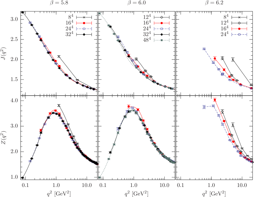
Figure 4.1: The ghost (upper panels) and gluon (lower panels) dressing functions for different lattice sizes as functions of momentum $q^{2}$. From left to right the panels show data at $\beta=5.8$, 6.0 and 6.2. Only data on fc gauge copies are shown here. Lines are drawn to guide the eye.

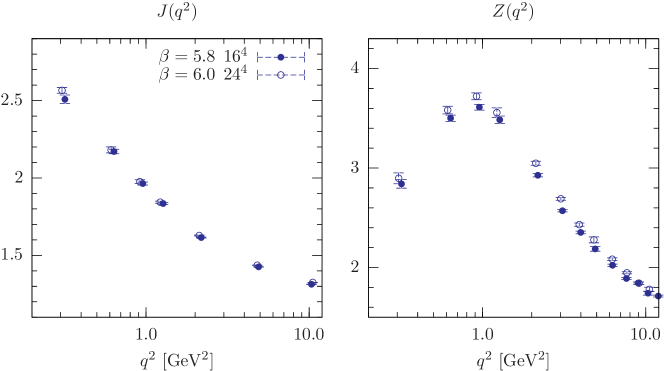
Figure 4.2: The ghost (left) and gluon (right) dressing functions are shown as functions of momentum $q^{2}$ at (approximately) fixed physical volume $V\approx(2.2\leavevmode\nobreak\ \textrm{fm})^{4}$. The data at $\beta=5.8$ (6.0) correspond to a lattice spacing of about $a=0.136\leavevmode\nobreak\ \textrm{fm}$ ($0.093\leavevmode\nobreak\ \textrm{fm}$). Only data obtained on fc gauge copies are shown here.

Discretization errors

Based on our chosen $\beta$ values and lattice sizes we can pick up equal physical volumes (with different coarseness) only approximately. Hence also the physical momenta are only approximately the same if the ghost and gluon dressing functions are compared at different $\beta$, i.e. at different lattice spacings. Therefore, it is difficult to analyze the systematic effect of changing $a$ if for both dressing functions this leads to small hidden variations in $q^{2}$. Consequently, in Fig. 4.2 we show data for the ghost and gluon dressing functions obtained at approximately the same physical volume $V\approx(2.2\leavevmode\nobreak\ \textrm{fm})^{4}$ for two different $a$ as functions of $q^{2}$. This allows us to disentangle by inspection a change of data due to varying $a$, given the physical dependence of the propagators on $q^{2}$. Looking at Fig. 4.2 one concludes that the gluon dressing function at the same physical momentum and volume increases with decreasing the lattice spacing. A similar effect (beyond error bars) is not observable for the ghost dressing function.

4.2.2 Asymmetric lattices cause strong systematic errors

Besides discretization and finite volume errors, there are also systematic effects involved using asymmetric lattice geometries. It could be tempting to use an asymmetric lattice such that in one direction, for example in time directions, the lattice extension is much longer than in all other directions. Going this way, one would tend to believe that much lower momenta can be studied compared to using symmetric lattice geometries at same computational costs. This approach has been pursued for example in SO05b ; OS05a ; SO05a ; OS05b aiming at the infrared behavior of the gluon propagator, in particular, at the determination of an infrared exponent for this propagator.

However, as a comparison of our data obtained either for symmetric or asymmetric lattice geometries suggests: “There is no free lunch!”. The more asymmetrically a lattice has been chosen, the larger are the systematic errors encountered by that. To make this point more clear, we have calculated both the ghost and gluon propagators not only on symmetric lattices as discussed above, but also on lattices of sizes $32^{3}\times 64$, $24^{3}\times 48$, $16^{3}\times 128$ and $24^{3}\times 128$ all at the same $\beta=6.0$ (see runs A-1 to A-4 in Table 4.1). The corresponding data are plotted in Fig. 4.3 together with those obtained on a $32^{4}$ and a $48^{4}$ lattice at the same value of $\beta$ (S-6, S-7 in Table 4.1). The lower panels of this figure show the corresponding dressing functions.

 

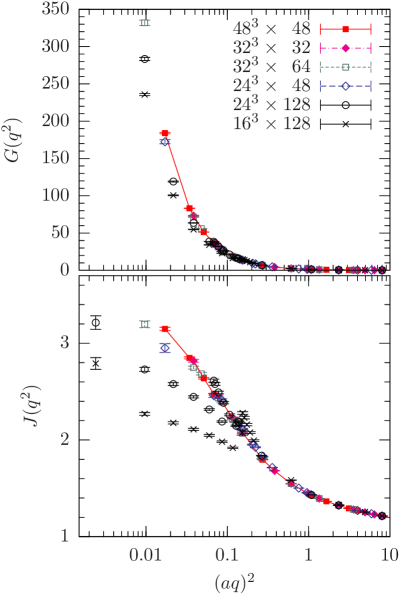
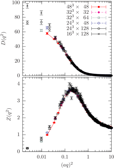
Figure 4.3: The ghost $G$ and gluon propagators $D$ (upper panels) and the corresponding dressing functions (lower panels) are shown at $\beta=6.0$ as functions of the momentum in lattice units. The data were obtained using different lattice geometries. Lines connecting data points for symmetric lattice geometries are drawn to guide the eye.

In Fig. 4.3 we clearly see that data obtained on a $16^{3}\times 128$ lattice suffer under the largest systematic errors in the low momentum region compared to the other data. In fact, the data on a $32^{3}\times 64$ lattice, shown using open squares in this figure, exhibit the smallest asymmetry effects. There only the data point at the lowest on-axis momentum for the ghost propagator is lower in tendency than an extrapolation including the lowest momentum data point referring to a $48^{4}$ lattice would give. For the gluon propagator this deviation is even smaller. Also for data on a $24^{3}\times 48$ lattice, shown using open diamonds, the asymmetry effect is small. There only the data point at the lowest on-axis momentum $k=(0,0,0,1)$ is lower (larger) than the corresponding result for the ghost (gluon) propagator on a $48^{4}$ lattice at the same momentum $a^{2}q^{2}(k)$. At larger momenta this effect is negligible within errors for these particular sets of data ($24^{3}\times 48$ and $32^{3}\times 64$ lattice).

Considering instead data generated on the lattices sizes $16^{3}\times 128$ and $24^{3}\times 128$, the results at the six or seven lowest momenta are significantly different to what is expected from the data obtained on symmetric lattices. A data inspection yields that the distorted momenta are only the on-axis momenta $k=(0,0,0,k_{t})$ allowed by a cylinder cut, but forbidden by a cone cut (see Sec. 4.1.4 for a definition of these cuts).

Similar systematic effects due to asymmetric lattice geometries have been reported recently for the gluon propagator in three-dimensional pure $SU(2)$ gauge theory CM [06], but in fact already in the well-known reference LSWP [99] for pure $SU(3)$ gauge theory. Therefore, extractions of an infrared exponent for the gluon propagator using only on-axis momenta on asymmetric lattices (see e.g. the references mentioned above) should be taken with reservations.

We note in passing that we also see in Fig. 4.3 points from asymmetric lattice geometries at not so small momenta which are slightly larger (lower) compared to those for the ghost (gluon) propagator on symmetric lattices. With respect to our discussion of finite volume effects above, we can, however, interpret this observation more generally as a finite volume effect caused by the lower spatial volumes of these asymmetric lattices.

4.2.3 Facing the problem of Gribov copies

Apart from the systematic effects inherent in any lattice study, it is known that the presence of Gribov copies may also causes a systematic error on the data of gauge-variant quantities. Below it is shown that this is indeed the case for the ghost propagator, while the influence on the gluon propagator seems to be negligible (i.e. hidden in the statistical noise). In SIMPS05d we have investigated this following the fc-bc strategy introduced in Sec. 4.1.3. For each set of fc and bc copies we have measured the ghost and gluon propagator to determine the systematic error caused through the Gribov ambiguity.

Estimating the number of gauge copies

   
   

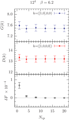
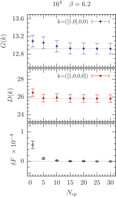
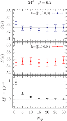
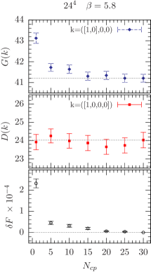
Figure 4.4: The upper panels show the ghost propagator $G(k)$ as average over two realizations $k=(1,0,0,0)$ and $k=(0,1,0,0)$ of the smallest lattice momentum, measured always on the best gauge copy among $N_{\textrm{cp}}{}$ copies. In the middle panel the same dependence is shown for the gluon $D(k)$ propagator, however, as average over all four permutations of $k=(1,0,0,0)$. The lower panels show the relative difference $\delta F=1-F^{\texttt{cbc}}/F^{\texttt{bc}}$ of the corresponding current best functional values $F^{\texttt{cbc}}$ to the value $F^{\texttt{bc}}$ of the overall best copy. The data are obtained at $\beta=6.2$ using the lattice sizes $12^{4}$ (left) and $16^{4}$ (right).

Figure 4.5: The same as in Fig. 4.5, however, the data refer to $\beta=5.8$ and 6.2 on a $24^{4}$ lattice.

In pursuing the fc-bc strategy, at some stage one has to figure out how large $N_{\textrm{cp}}{}$ has to be approximately. This does not mean that we can be confident that the set of best copies then in any respect represents the real ones, i.e. those which give rise to the absolute maximum of the gauge functional $F_{U}[g]$ (Eq. (3.14)) for each $U$. It turns out, however, that for each gauge-variant observable there exists a certain $N_{\textrm{cp}}{}$ that warrants the convergence of that particular observable.

Numerically, it turns out that the dependence of the ghost propagator on the choice of the best copy is most severe for the smallest momentum. In addition, this sensitivity depends on the lattice size and $\beta$. Therefore we studied first the dependence of the ghost and gluon propagators at lowest momentum (ignoring the cone cut) on the (same) best copies as function of the number of gauge copies $N_{\textrm{cp}}{}$ under inspection. This was done at $\beta=6.2$ where we used $12^{4}$, $16^{4}$ and $24^{4}$ lattices. The number of thermalized configurations used for these three lattice sizes are given in [Table 4.1: F-2 to F-4]. To check the dependence on $\beta$ also a simulation at $\beta=5.8$ on a $24^{4}$ lattice was performed [Table 4.1: F-1].

The results of this investigation are shown in Fig. 4.5 and 4.5. While there the ghost propagator is shown as an average over the two realizations $k=(1,0,0,0)$ and $k=(0,1,0,0)$ of the smallest lattice momentum $a^{2}q^{2}(k)$, the gluon propagator has been averaged over all four non-equivalent realizations. Note that $D(k)=D(-k)$.

In Fig. 4.5 and 4.5 it is clearly visible that the expectation value of the gluon propagator does not change within errors as $N_{\textrm{cp}}{}$ increases, independently from the lattice size and $\beta$. Contrarily, the ghost propagator at $\beta=5.8$ on a $24^{4}$ lattice saturates (on average) if calculated on the best among $N_{\textrm{cp}}{}=15$ gauge copies. At $\beta=6.2$ the number of necessary gauge fixings attempts reduces to $5\leq N_{\textrm{cp}}{}\leq 10$ on a $16^{4}$ and $24^{4}$ lattice. On the $12^{4}$ lattice a small impact of Gribov copies is visible, namely $1<N_{\textrm{cp}}{}\leq 5$ is sufficient for convergence. The lower panels of Fig. 4.5 and 4.5 show the average of the relative difference $\delta F=1-F^{\texttt{cbc}}/F^{\texttt{bc}}$ of the corresponding (current best) functional value $F^{\texttt{cbc}}$ to the value $F^{\texttt{bc}}$ of the overall best copy after $N_{\textrm{cp}}{}=20$, respectively $N_{\textrm{cp}}{}=30$, attempts. This may serve as an indicator how large $N_{\textrm{cp}}{}$ has to be, on average, for the chosen algorithm to find a maximum of $F$ close to the global one. In Table 4.1 the respective numbers $N_{\textrm{cp}}{}$ for the different simulations are given.

Gribov copies may cause systematic errors

Having specified the necessary amount of gauge copies we focus now on the influence the Gribov ambiguity might have on the gluon and ghost propagators. To investigate this a combined study of the gluon and ghost propagators on the same sets of fc and bc representatives of our thermalized gauge field configurations has been performed (see SIMPS05d ). This has allowed us to assess the importance of the Gribov copy problem for the ghost propagators in the low-momentum region.

 

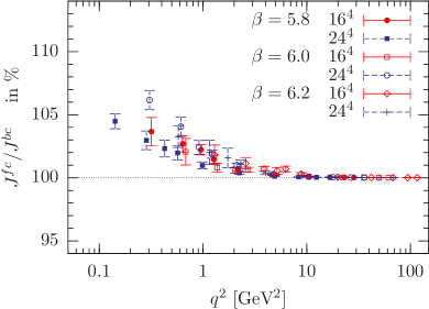
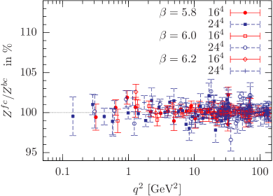
Figure 4.6: The ratios $J^{\texttt{fc}}/J^{\texttt{bc}}$ and $Z^{\texttt{fc}}/Z^{\texttt{bc}}$ of ghost (l.h.s.) and gluon (r.h.s.) dressing functions, respectively, vs. momentum $q^{2}$. $J^{\texttt{fc}}$ and $Z^{\texttt{fc}}$ refer to values determined on first (fc) gauge copies, whereas $J^{\texttt{bc}}$ and $Z^{\texttt{bc}}$ to those on best (bc) copies. The ratios were calculated using jackknife.

To be specific we have generated different sets of quenched gauge configuration using the inverse coupling constants $\beta=5.8$, 6.0 and 6.2 and the lattice sizes $16^{4}$ and $24^{4}$. The corresponding entries in Table 4.1 are S-1, S-2, S-4, S-5, S-8 and S-9. Following our fc-bc strategy, each gauge configuration $U$ has been fixed to Landau gauge a number of $N_{\textrm{cp}}{}$ times using over-relaxation and starting always from an random gauge copy of $U$. Then for each $U$ the first (fc) and the best (bc) gauge copy (among $N_{\textrm{cp}}{}$ copies) form the two ensembles for measurements of the ghost and gluon propagator.

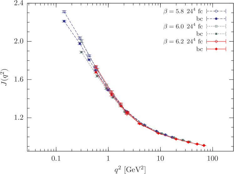
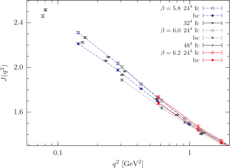
Figure 4.7: The ghost dressing function determined on first (fc) and best (bc) gauge copies vs. momentum $q^{2}$. Only data on a $24^{4}$ lattice are shown here at three different values of $\beta$. Lines connecting data points belonging to the same $\beta$ are drawn to guide the eye.

Figure 4.8: The same as in Fig. 4.8, but focussing on a lower range of momenta. In addition, fc data on a $32^{4}$ lattice at $\beta=5.8$ and on a $48^{4}$ lattice at $\beta=6.0$ are shown.

In Fig. 4.6 we illustrate the effect of the different Gribov copies by plotting the ratios $J^{\texttt{fc}}/J^{\texttt{bc}}$ and $Z^{\texttt{fc}}/Z^{\texttt{bc}}$ of the ghost and gluon dressing functions, respectively. $J^{\texttt{fc}}$ and $Z^{\texttt{fc}}$ refer to values determined on first (fc) gauge copies, whereas $J^{\texttt{bc}}$ and $Z^{\texttt{bc}}$ to those on best (bc) copies. Obviously, in Fig. 4.6 there is no influence visible for the gluon propagator within the statistical noise. On the contrary, for the ghost propagator the Gribov problem can cause $O\left(5\%\right)$ deviations in the low-momentum region ($q<1\leavevmode\nobreak\ \mbox{GeV}$). For better gauge copies the ghost dressing function becomes less singular in the infrared. This can also be seen in Fig. 4.8 and 4.8 where both fc and bc data for the ghost propagator are shown.

A closer inspection of the data in Fig. 4.6 and 4.8 indicates that the influence of Gribov copies on the ghost propagator becomes weaker for increasing the lattice size. In fact, comparing in Fig. 4.6 ratios for the ghost dressing function at $q<1\leavevmode\nobreak\ \textrm{GeV}$, the rise at $\beta=6.0$ is obviously larger than that at $\beta=5.8$. In both cases the data are from simulations on a $24^{4}$ lattice. Thus, it seems that by increasing the physical volume (lower $\beta$) the effect of the Gribov ambiguity gets smaller if the same physical momentum is considered. This we can also deduce from Fig. 4.8 and 4.8. There obviously the difference between $J^{\texttt{fc}}$ and $J^{\texttt{bc}}$ at lower momentum reduces when $\beta$ decreases. We think this observation is not biased by a too small number $N_{\textrm{cp}}{}$ of inspected gauge copies since, judging from Fig. 4.5 and 4.5, $N_{\textrm{cp}}{}=40$ as specified in Table 4.1 seems to be on the safe side. However, in a future project one should definitely check the ratios on a $32^{4}$ lattice at $\beta=6.2$ to eliminate the last doubts.

We conclude: the ghost propagator systematically depends on the choice of Gribov copies, while the impact on the gluon propagator is not resolvable within our statistics. However, there are indications that the dependence on Gribov copies decreases with increasing physical volume. This is also in agreement with the data listed in the two lattice studies BIMMP [04]; Cuc [97] of the $SU(2)$ ghost propagator $G$, while it is not explicitly stated there. In fact, in Ref. BIMMP [04] the ratio $G^{\texttt{fc}}/G^{\texttt{bc}}$ at $\beta=2.2$ on a $8^{4}$ lattice is larger than that on a $16^{4}$ lattice at the same physical momentum. In BBMPM [05] similar indications have been found for $SU(2)$ taking non-periodic $Z(2)$ transformations into account.

Note also that this observation is in agreement with a recent claim by Zwanziger according to which in the infinite volume limit averaging over gauge configurations in the Gribov region should lead to the same result as averaging over configurations in the fundamental modular region Zwa [04].

4.3 The infrared behavior of gluon and ghost propagator in the quenched and unquenched case

After discussing different systematic effects on the gluon and ghost propagators or on the corresponding dressing functions we concentrate now on the infrared behavior. Thereby, however, we shall study a further systematic effect, namely the change of data at lower momenta due to unquenching the theory. As we shall see below, this change is negligible for the ghost propagator, but conspicuously large for the gluon propagator at not so small momenta.

4.3.1 The gluon propagator

From the material presented above it is clear that the gluon propagator in Landau gauge does not suffer from the Gribov ambiguity, at least in the momentum range considered. Therefore, if we restrict ourselves in the following to consider only fc gauge copies, the systematic effect involved will stay most probably within statistical errors. This has the advantage of allowing us to use data obtained on larger lattice sizes even though they have been collected only from the ensemble of fc gauge copies.

Just as a reminder, in our simulations the gluon propagator was determined for all momenta at once. However, only a subset of data was used for the final analysis. For details see Sec. 4.1.4 where our selection of momenta is specified. The way how lattice momenta are connected to physical ones is discussed in Sec. 4.1.5. Beside this, it is also clear that all data obtained in lattice simulations have to be subject to a renormalization, discussed in Sec. 3.3.4. In the following the data presented for the gluon and ghost dressing functions, $Z$ and $J$, are renormalized such that at the renormalization point $\mu=4\leavevmode\nobreak\ \textrm{GeV}$ they are fixed to $Z(\mu^{2},\mu^{2})=J(\mu^{2},\mu^{2})=1$.

The quenched gluon propagator

In Fig. 4.10 the dressing function of the gluon propagator is collected from data at different $\beta$ values as a function of the (physical) momentum $q^{2}$. Based on the experiences gained in previous sections only data obtained on larger lattice sizes are presented there. Beside of a cylinder cut applied to all data, a cone cut has been imposed to data related only to the lattice sizes $16^{4}$ and $24^{4}$. Since finite volume errors on the larger lattices are small, it is not necessary to impose this cut there.

Obviously, the data surviving all cuts lie along a smooth curve which not only is nonperturbatively enhanced around $q=1\leavevmode\nobreak\ \textrm{GeV}$ as expected, but also decreases in a sufficiently large range of low momenta. Therefore, it appears natural trying to fit the ansatz

$$f_{D}\left(q^{2}\right)=A_{D}\cdot\left(q^{2}\right)^{\kappa_{D}}$$ (4.3)

to the data at lower momenta. As mentioned above, from studies of truncated DSE for the gluon propagator an infrared exponent $\kappa_{D}=2\kappa$ with $\kappa\approx 0.595$ is expected to describe the infrared behavior LvS [02]; Zwa [02].

We have tried to fit this ansatz to the data by imposing a upper-momentum cut $q^{2}<q^{2}_{i}$ that has been varied. The parameters $A_{D}$ and $\kappa_{D}$ extracted and the values of $q^{2}_{i}$ used are listed in Table 4.3. As can be seen in this table shifting $q^{2}_{i}$ to larger momenta a fit with ansatz (4.3) becomes worse. The parameters of our best fit to the data have been given in bold letters and in Fig. 4.10 we have plotted the corresponding fitting function $f_{D}(q^{2})$. Although this fit supports the conjecture of an infrared vanishing gluon propagator our value of $\kappa_{D}=0.83(2)$ is lower than expected from the DSE studies. However, there is a tendency for $\kappa_{D}$ to rise as the interval of momenta, contributing to the fit, is shrinking towards the infrared. Therefore, we cannot exclude the expected infrared behavior to become realized at much lower momenta.

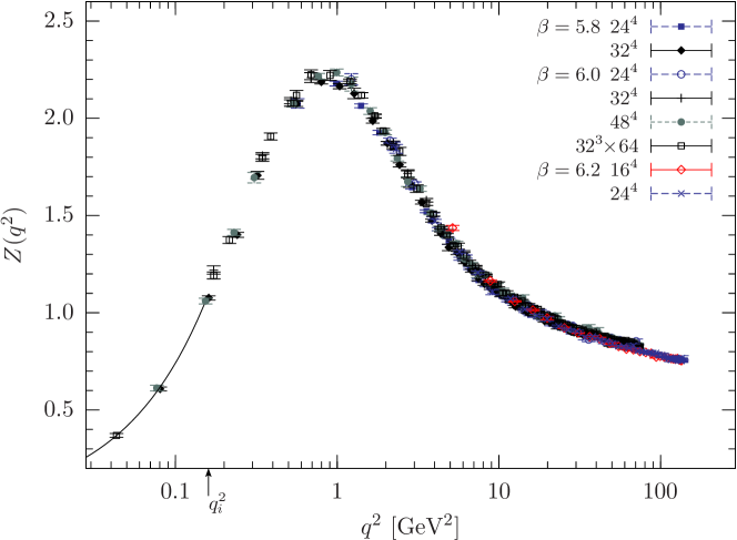
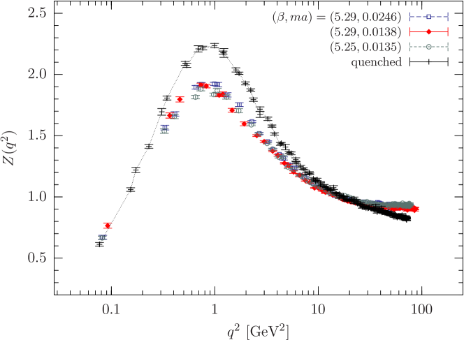
Figure 4.9: The dressing function of the gluon propagator renormalized at $\mu=4$ GeV is shown as a function of momentum $q^{2}$ using various lattice sizes. All data have been obtained from first gauge copies in quenched simulations (see Table 4.1). The line refers to an infrared fit on the data as explained in the text. The momentum $q^{2}_{i}$ marks the largest momentum used for this fit.

Figure 4.10: The same as in Fig. 4.10, including now data obtained on first gauge copies of unquenched configurations (see D-2 to D-4 in Table 4.2). For comparison some quenched data at $\beta=6.0$ [Table 4.1: S-6, S-7] have been included in this figure as well. A dotted line connecting quenched data is drawn to guide the eye.

The unquenched gluon propagator

Beside of our measurements in the quenched approximation we have also determined the gluon propagator on gauge-fixed copies (gauge-fixed only once) of dynamical gauge configurations specified in Table 4.2. The results of the corresponding dressing functions are shown in Fig. 4.10. With respect to finite volume effects reported above for the quenched case we have plotted in this figure only data obtained on a $24^{3}\times 48$ lattice, nevertheless for three different pairs of $\beta$ and $\kappa$ (see D-2, D-3 and D-4 in Table 4.2). Note, the data related to the $16^{3}\times 32$ lattice (D-1) turn out to exhibit similar finite volume effects as reported for quenched configurations.

In order to perform a comparison with our quenched data with the greatest of ease some of the quenched data have been included in this figure as well, namely the results at $\beta=6.0$ associated with a $32^{4}$ and a $48^{4}$ lattice. The lattice spacing associated with this $\beta$ is comparable to those of the dynamical configurations. As above the dressing functions were renormalized at $\mu=4\leavevmode\nobreak\ \textrm{GeV}$.

As can be seen from Fig. 4.10, the unquenching effect becomes clearly visible for the gluon dressing function, in particular around $q^{2}\simeq 1\textrm{GeV}^{2}$. There the non-perturbative enhancement, characteristic to this function, is drastically reduced compared to the quenched data ($ma=\infty$). It also becomes softer as the quark mass is decreasing, even though this is a small effect. This has been observed also in recent lattice computations of the gluon propagator using configurations generated with dynamical AsqTad-improved staggered quarks BHL⁺ [04] as well as from unquenching studies for the ghost and gluon propagators within the DSE approach FAC⁺ [06]; FWC [05]; FA [03]. We refer also to recent lattice studies with dynamical Kogut-Susskind and Wilson fermions FN05a ; FN05b . The difference between quenched and unquenched data in the ultraviolet asymptotic tail is consistent with what is expected from perturbation theory (see Sec. 1.3.4).

Unfortunately, the amount of data collected for momenta in the range $q^{2}<1\textrm{GeV}^{2}$ does not allow for a fit to the ansatz given in Eq. (4.3). Intuitively, one may guess, looking at the low–momentum tendency of the unquenched data points in Fig. 4.10, that in the infrared the unquenched gluon dressing function might match that of the quenched case.

4.3.2 The ghost propagator

In the discussions of different systematic effect we have found that the Gribov ambiguity has an influence on the ghost propagator. Nevertheless, in Fig. 4.8 we have also seen that even though the effect is visible in the data, the systematic error one would encounter by neglecting the Gribov copy problem is not that large. Since at present our data collected on fc gauge copies cover much lower momenta, we analyze in the following only those. Incidentally, this also allows for a fair comparison of our quenched and unquenched data.

The quenched ghost propagator

The ghost dressing function has been determined on the same gauge configurations as that of the gluon propagator discussed above. However, the list of momenta studied is much shorter than that of the gluon propagator. Anyway, we have tried to cover as much as possible the whole range of momenta with special focus on the infrared region. The selection of momenta was guided by the cylinder cut and for smaller lattices sizes sharpened by the cone cut.

Our results for the quenched ghost dressing function are shown in Fig. 4.12. As for the gluon dressing function we used $\mu=4\leavevmode\nobreak\ \textrm{GeV}$ as renormalization point such that $J(\mu^{2},\mu^{2})=1$. The data all lie along a smooth curve. Thus we may conclude that both cylinder and cone cut work well also for the ghost propagator. Note that in contrast to the gluon dressing function here a cone cut has not been imposed on a $24^{4}$ lattice.

As expected the ghost dressing function seems to diverge with decreasing momenta and we have tried to fit the infrared behavior again by an ansatz motivated through the mentioned studies of the ghost propagator within the DSE approach. To be specific, we fitted the ansatz

$$f_{G}\left(q^{2}\right)=A_{G}\cdot\left(q^{2}\right)^{-\kappa_{G}}$$ (4.4)

to the data at lower momenta. From the mentioned studies one usually expects to get $\kappa_{G}\approx 0.595$ LvS [02]; Zwa [02]. Even more importantly, one expects $\kappa_{G}=2\kappa_{D}$ to hold. See below for a discussion about that.

The ansatz (4.4) has been fitted to our data by imposing an upper momentum cut $q^{2}<q^{2}_{i}$. However, in contrast to the gluon dressing function, here the parameter $A_{G}$ and $\kappa_{G}$ turn out to be more robust against shifting $q^{2}_{i}$. This can be seen in Table 4.3 where the parameters obtained are given. In Fig. 4.12 we show the corresponding fitting function. Even though data at the lowest three momenta available on a $24^{4}$ lattice are shown in Fig. 4.12 they do not contribute to the fit. We also have used data only at $\beta=6.0$, because including data at $\beta=5.8$ in the fit makes it even worse.

Our fits to the data suggest that $\kappa_{G}=0.20(1)$ which is far away from values larger than 0.5. Therefore, we cannot confirm the expected infrared exponent $\kappa\approx 0.595$ on the basis of our data. Also the not so small values found for $\chi^{2}/\textrm{ndf}$ indicate that the power ansatz (4.4) seems to be not reasonable for the range of momenta considered. Note also that the linear rise of the data in Fig. 4.12 (momentum log-axis) for decreasing momenta suggest the ghost dressing function might diverge logarithmically at least in the considered range of momenta. However, we do not know arguments that would support this.

Together with our results for the gluon dressing function we can neither confirm the expected values of the infrared exponents nor that there the relation

$$\kappa_{D}-2\kappa_{G}=\Delta$$

holds with $\Delta=0$, at least from the data available to us. Our fits yield $\Delta\approx 0.43$. Furthermore, one should remark here that even though we have fitted the Ansätze (4.4) and (4.3) to the corresponding dressing functions, the fits are quite unstable. For the ghost dressing function the fitting function does even not really describe the tendency of data towards the infrared (see Fig. 4.12).

	ghost			gluon
$q_{i}^{2}$	$A_{G}$	$\kappa_{G}$	$\chi^{2}/\textrm{ndf}$	$A_{D}$	$\kappa_{D}$	$\chi^{2}/\textrm{ndf}$
0.16	–	–	–	5.0(3)	0.83(2)	1.2
0.20	–	–	–	5.1(3)	0.84(3)	3.2
0.25	1.55(5)	0.20(2)	3.8	4.4(2)	0.77(3)	8.6
0.35	1.53(3)	0.20(1)	4.0	4.0(1)	0.72(2)	9.8
0.55	1.53(1)	0.20(1)	3.1	3.3(1)	0.62(3)	38.0
0.70	1.51(1)	0.21(1)	4.3	–	–	–

Table 4.3: Parameter extracted corresponding to the fitting Ansätze (4.4) and (4.3) for the ghost and gluon dressing function, respectively. The first row specifies the upper-momentum cutoff $q^{2}_{i}$, i.e. $q^{2}<q^{2}_{i}$. Bold letters indicate parameters used for the fitting function shown in Fig. 4.12 and 4.10, respectively.

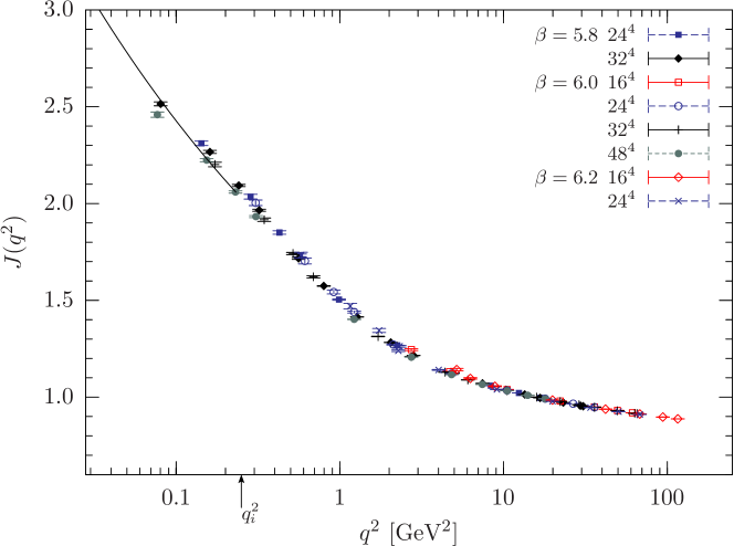
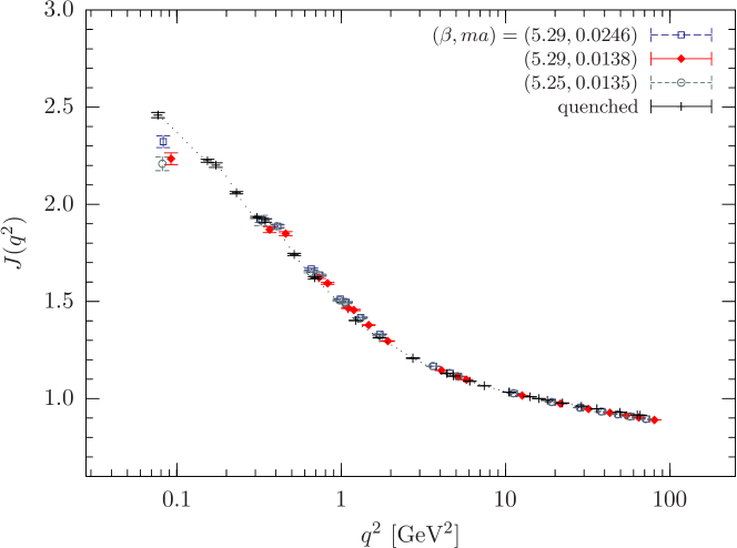
Figure 4.11: The dressing function of the ghost propagator renormalized at $\mu=4\leavevmode\nobreak\ \textrm{GeV}$ is shown as a function of momentum $q^{2}$ using data from various lattice sizes. All data have been obtained from first gauge copies in quenched simulations (see Table 4.1). The line refers to an infrared fit to the data as explained in the text. The momentum $q^{2}_{i}$ marks the largest momentum used for this fit.

Figure 4.12: The same as in Fig. 4.12, however, most of the data are obtained on first gauge copies of unquenched configurations using a $24^{3}\times 48$ lattice (see D-2 to D-4 in Table 4.2). For comparison, some quenched data at $\beta=6.0$ [Table 4.1: S-6, S-7] have been included into this figure as well. A dotted line connecting quenched data is drawn to guide the eye. The unquenched data at lowest momentum refer to the lattice momentum $k=(0,0,0,1)$ on a $24^{3}\times 48$ lattice and are most probably affected by lattice-asymmetry effects.

The unquenched ghost propagator

In Fig. 4.12 we present our full QCD result for the ghost dressing functions. There we have not discard data at the lowest on-axis momentum in order to illustrate the systematic effect encountered through the asymmetric lattice geometry. For comparison, selected data of the quenched case (i.e. for infinite quark mass) are also shown, namely those on $32^{4}$ and $48^{4}$ lattice at $\beta=6.0$. As in the quenched case the dressing function has been renormalized such that $J(\mu^{2},\mu^{2})=1$ at $\mu=4\leavevmode\nobreak\ \textrm{GeV}$.

In contrast to the gluon dressing function, in Fig. 4.12 the unquenching effect is very small. In the ultraviolet the unquenched data are slightly lower and at lower momenta they are slightly larger than the quenched data, but altogether the effect stays within error bars and thus can be neglected in the region of momenta considered here. Negligible unquenching effect are in agreement with what is expected from unquenching studies for the ghost and gluon propagators within the DSE approach FAC⁺ [06]; FA [03]. We refer also to recent lattice studies with dynamical Kogut-Susskind and Wilson fermions FN05a ; FN05b . Thus, even though we cannot confirm the predicted infrared exponent (from the DSE studies), we affirm that the influence of fermions on the infrared behavior of the ghost propagator is negligible.

4.4 The running coupling and the ghost-gluon vertex

After extensively reporting on results obtained for the gluon and ghost dressing functions, now we focus on the running coupling constant $\alpha_{s}(q^{2})$. As explained in Sec. 2.2.2, $\alpha_{s}(q^{2})$ may be defined by a renormalization-group-invariant combination of the gluon and ghost dressing functions (Eq. (2.10))

$$\alpha_{s}(q^{2})=\alpha_{s}(\mu^{2})Z(q^{2},\mu^{2})J^{2}(q^{2},\mu^{2}).$$ (4.5)

Remember that this definition relies on the assumption that the ghost-gluon vertex in Landau gauge stays bare also beyond perturbation theory. Below we give numerical evidence confirming $\widetilde{Z}_{1}\approx 1$ in a MOM scheme where the gluon momentum equals zero. This we show for both the quenched and unquenched case of $SU(3)$. Similar results indicating this, directly CMM [04] and indirectly BCLM [04], were presented in studies of the quenched $SU(2)$ gauge theory, but also in semiperturbative calculations within the DSE approach SMWA [05].

4.4.1 Results for the running coupling constant

Based on our data for the renormalized gluon and ghost dressing functions, we have estimated the product in Eq. (4.5) using the bootstrap method with drawing 500 random samples. Since the ghost-gluon-vertex renormalization constant $\widetilde{Z}_{1}$ has been set to one, there is an overall normalization factor which has been fixed by fitting the data for $q^{2}>q^{2}_{c}$ to the well-known perturbative results of the running coupling $\alpha_{\texttt{2-loop}}$ at 2-loop order (see also BCLM [04]). Defining $x\equiv q^{2}/\Lambda^{2}_{\texttt{2-loop}}$, the 2-loop running coupling is given by

$$\alpha_{\texttt{2-loop}}(x)=\frac{4\pi}{\beta_{0}\ln x}\left\{1-\frac{2\beta_{1}}{\beta^{2}_{0}}\frac{\ln(\ln x)}{\ln x}\right\}.$$ (4.6)

The $\beta$-function coefficients $\beta_{0}$ and $\beta_{1}$ have been defined in Eq. (1.45a) and (1.45b). They are independent of the renormalization prescription. The value of $\Lambda_{\texttt{2-loop}}$ has been fixed by the same fit. The lower bound $q^{2}_{c}$ has been chosen such that an optimal value for $\chi^{2}/{\textrm{ndf}}$ has been achieved.

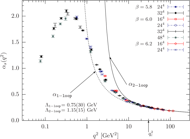
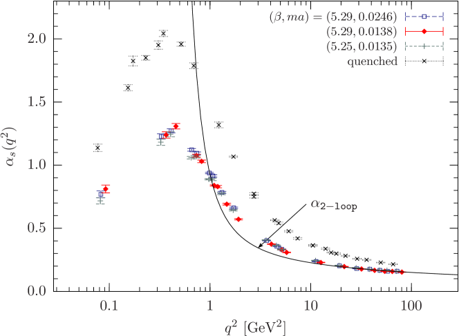
Figure 4.13: The running coupling $\alpha_{s}(q^{2})$ as a function of the momentum $q^{2}$. The data refer to first (fc) gauge copies of quenched configurations.

Figure 4.14: The running coupling $\alpha_{s}(q^{2})$ as a function of momentum $q^{2}$ determined on gauge-fixed configurations in the unquenched case. For comparison, we also show quenched data (crosses) obtained at $\beta=6.0$ on a $32^{4}$ and $48^{4}$ lattice.

The results are shown in Fig. 4.14. There also the 1-loop contribution is shown where we used the lower bound $q^{2}_{c}=50\leavevmode\nobreak\ \textrm{GeV}^{2}$. The best fit of the 2-loop expression to the data gives $\Lambda_{\texttt{2-loop}}=1.15(15)\leavevmode\nobreak\ \textrm{GeV}$ ($\chi^{2}/{\textrm{ndf}}=7.5$), while $\Lambda_{\texttt{1-loop}}=0.75(30)\leavevmode\nobreak\ \textrm{GeV}$ is obtained ($\chi^{2}/{\textrm{ndf}}=5.2$) using just the 1-loop part. For the 2-loop expression we used $q^{2}_{c}=30\leavevmode\nobreak\ \textrm{GeV}^{2}$. The value for $\Lambda_{\texttt{2-loop}}$ is similar within errors to the $SU(2)$ result given in Ref. BCLM [04]. Note that we have imposed again a cone cut to data obtained on a $16^{4}$ and $24^{4}$ lattice.

Approaching the infrared limit in Fig. 4.14 one clearly sees $\alpha_{s}(q^{2})$ increasing for $q^{2}>0.4$ GeV². However, after passing a maximum at $q^{2}\approx 0.4$ GeV² $\alpha_{s}(q^{2})$ decreases again. The same behavior is found on our sets of dynamical gauge configurations. These results are presented in Fig. 4.14 where quenched data ($\beta=6.0$: $32^{4}$ and $48^{4}$) are also shown for comparison. In fact, looking at Fig. 4.14 we clearly see that the same turnover, as found in the quenched case, can be assumed for the unquenched case, even though the data at the lowest (on-axis) momenta have to be taken with special care. (See our discussion concerning systematic effects due to asymmetric lattices.) Therefore, the data points at $q^{2}\simeq 0.1\mbox{GeV}^{2}$ have to be checked carefully on larger symmetric lattices, in order to eliminate the last doubts.

We observe a quite clear unquenching effect for $\alpha_{s}(q^{2})$ extending from the perturbative range down to the infrared region. We think that this is caused in the majority due to unquenching effects as found for the gluon propagator in Sec. 4.3.1.

Note that a similar infrared behavior of $\alpha_{s}(q^{2})$ as presented here has been observed in other lattice studies FN04a ; FN04b . But opposed to Ref. FN04b we argue that the existence of a turnover is independent on the choice of Gribov copies. In fact, qualitatively we have found the same behavior if $\alpha_{s}(q^{2})$ is calculated on bc gauge copies. To illustrate this, in Fig. 4.15 we show the corresponding data extracted in bc copies. There we have not impose the cone cut on data associated with the $24^{4}$ lattice. Obviously, $\alpha_{s}(q^{2})$ decreases also in this case and a decreasing running coupling constant is not due to restricting to fc gauge copies.

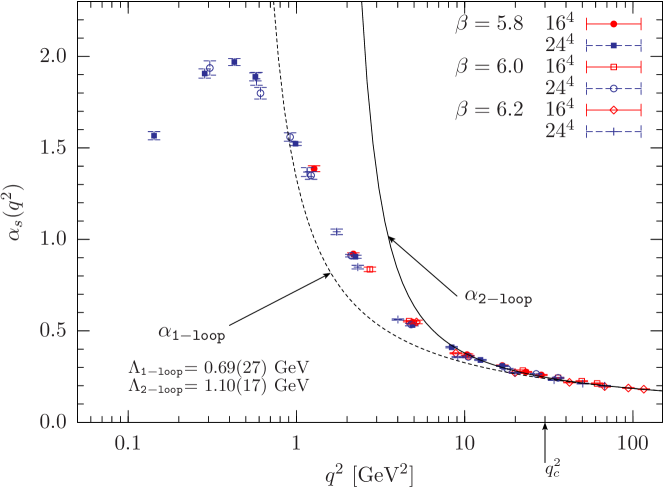
Figure 4.15: The running coupling $\alpha_{s}(q^{2})$ as a function of momentum $q^{2}$ determined on best (bc) gauge copies of quenched configurations.

The values for $\Lambda_{\texttt{1-loop}}$ and $\Lambda_{\texttt{2-loop}}$ are the same within error bars as obtained on fc gauge copies.

We should remark here that our observation of an infrared decreasing running coupling is in agreement with recent studies of DSE results obtained on a torus FAR [02]; FA [02]; FGA [06]; FP [06]. In those studies $\alpha_{s}(q^{2})$ was shown to tend to zero for $q^{2}\to 0$ in one-to-one correspondence with what one finds on the lattice. This would indicate very strong finite-size effects and a slow convergence to the infinite-volume limit. However, on the lattice we do not find any indication for such a strong finite-size effect, except the convergence to the infinite-volume limit would be extremely slow. An alternative resolution of this problem has been proposed by Boucaud et al. B⁺05b . These authors have argued that the ghost-gluon vertex in the infrared might contain $q^{2}$-dependent contributions which could modify the DSE results for the mentioned propagators. Note, however, that recent DSE studies of the ghost-gluon vertex did not provide hints for such a modification SMWA [05]; AFLE [05]. Thus, at present there seems to be no solution of the puzzle.

For completeness we mention that running coupling constants decreasing in the infrared have also been found in lattice studies of the 3-gluon vertex BLM⁺98a ; B⁺ [03] and the quark-gluon vertex SK [02].

4.4.2 The vertex renormalization constant

For discussing the infrared behavior of the running coupling it is interesting to have an independent check of whether the renormalization constant $\widetilde{Z}_{1}$ really stays constant for all renormalization points. Remember, this is always assumed if renormalization-group invariance is demonstrated for the product of gluon and ghost dressing functions in Eq. (4.5) and hence is important for this particular definition of a nonperturbative running coupling constant.

In principle the finiteness of $\widetilde{Z}_{1}$ has to be checked in each renormalization scheme separately. A first attempt to calculate $\widetilde{Z}_{1}$ on the lattice was made in CMM [04] for quenched $SU(2)$ gauge theory using the particular renormalization scheme of zero gluon momentum (see also BCLM [04] for an indirect determination). To confirm these findings also for the gauge group $SU(3)$ in the quenched and unquenched case, we have used the same renormalization scheme as in CMM [04] for a calculation of $\widetilde{Z}_{1}$. The necessary observable to be estimated on the lattice has been derived in Sec. 3.3.5 (see Eq. (3.44)). Since this is a combination of MC averages for the ghost and gluon propagators and for the 3-point function $G^{abc}_{\mu}$ of gluon, ghost and anti-ghost fields (see Eq. (3.43) and (3.45)) we used again the Bootstrap method to estimate errors.

Our data for the inverse of $\widetilde{Z}_{1}$ from quenched simulations are shown in Fig. 4.17. To simplify matters, we have restricted ourselves to present only data obtained on the largest lattice available at $\beta=5.8$ and 6.0. For data on smaller lattices we refer to our recent conference proceeding SIMPS [06]. The data there agree within errors with those presented here.

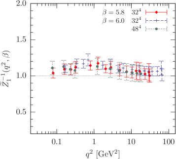
Figure 4.16: The (inverse of the) ghost-gluon-vertex renormalization constant $\widetilde{Z}_{1}$ is shown versus the momentum $q^{2}$. The data refer to quenched simulations at $\beta=5.8$, and 6.0 using a $32^{4}$ and $48^{4}$ lattice. Only data on fc gauge copies are available.

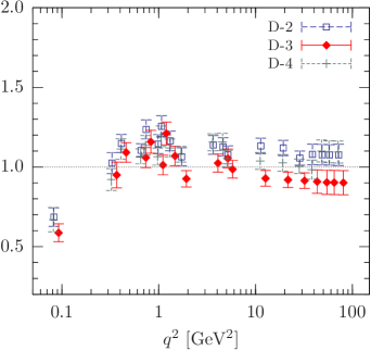
Figure 4.17: The same as in Fig. 4.17, but the data are obtained on unquenched gauge configurations using a $24^{3}\times 48$ lattice. The points at the lowest momentum refer to the on-axis momentum $k=(0,0,0,1)$ on that lattice. Labels refer to the parameters $\kappa$ and $\beta$ given in Table 4.2.

In Fig. 4.17 we clearly see that $\widetilde{Z}_{1}$ stays constant in the region of momenta considered. This holds for the data at both $\beta=5.8$ and $\beta=6.0$. Only a slight variation is visible in the interval $0.3\leavevmode\nobreak\ \textrm{GeV}^{2}\leq q^{2}\leq 2\leavevmode\nobreak\ \textrm{GeV}^{2}$, but this remains within error bars. The same can be concluded from our data obtained on unquenched configurations using a $24^{3}\times 48$ lattice. These are shown in Fig. 4.17 for three different settings of $\kappa$ and $\beta$ (see the data set entries D-2, D-3, D-4 in Table 4.2). For all three cases, the renormalization constant $\widetilde{Z}_{1}$ does not differ beyond error bars from being constant, but there is a certain trend of deviation from unity which systematically depends on the parameter setting $(\beta,\kappa)$.

For each tuple there is also one data point at the lowest (on-axis) momentum available on a $24^{3}\times 48$ lattice (i.e. $k=(0,0,0,1)$) which is much lower than unity. This particular deviation we also find at the lowest on-axis momentum in our data obtained on quenched configurations at $\beta=6.0$ when using a $24^{3}\times 48$ and $32^{3}\times 64$ lattice (not shown). Since the data taken in simulations on a $48^{4}$ lattice at the same $\beta$ do not show such a deviation, see Fig. 4.17, this effect is most probably caused by the asymmetric lattice geometry as it was reported also for the propagators in Sec. 4.2.1. Data at this momentum on an asymmetric lattice would have to be ignored. To eliminate the last doubts we have also inspected our data for $\widetilde{Z}_{1}$ obtained at the lowest on-axis momenta on a $24^{3}\times 128$ lattice at $\beta=6.0$. We find for these data that this particular deviation is even more dramatic. Hence, asymmetric lattices are not appropriate for studying the ghost-gluon-vertex renormalization constant at very low momentum.

In summary, our results for the quenched and unquenched case of $SU(3)$ are in full agreement with those presented in CMM [04] for the case of $SU(2)$. Even though there is a weak deviation of $\widetilde{Z}_{1}$ from being constant this will not have a dramatic influence on the running coupling. Together with our data for the running coupling we can thus confirm that in the special MOM scheme considered here (gluon momentum equals zero) the product in Eq. (4.5) is indeed renormalization-group invariant and thus defines a nonperturbative running coupling which monotonously decreases with decreasing momentum in the range $q^{2}<0.3\leavevmode\nobreak\ \textrm{GeV}^{2}$.

It is worthwhile to continue the lattice calculations of $\widetilde{Z}_{1}$ using other renormalization schemes, for example the scheme with a symmetric subtraction point. This has been undertaken in a recent study SMWA [05] where a semiperturbative calculation of $\widetilde{Z}_{1}$ within the DSE approach has been presented. There are also data shown for the same renormalization scheme as used by us which qualitatively agree with our results and those in CMM [04].

Chapter 5 Confinement criteria under the lattice microscope

[0,l,H,] ere we discuss data for the $SU(3)$ Landau gauge gluon and ghost propagators in the light of the Gribov-Zwanziger horizon condition and the Kugo-Ojima confinement scenario. For the latter we also present recent data for the function $u(q^{2})$ whose zero-momentum limit $u(q^{2}=0)$, the Kugo-Ojima confinement parameter, is expected to be minus one. Note that our lattice estimate of the function $u(q^{2})$ is (to our knowledge) the first presented in the literature. The data have been renormalized using a minimization process, developed here for the first time. We show that, under the assumption the ghost dressing function being divergent in the infrared, the function $u(q^{2})$ will reach minus one at zero momentum. Finally, we discuss numerical evidence for the gluon propagator violating reflection positivity explicitly.

5.1 Is the Gribov-Zwanziger horizon condition satisfied?

The Gribov–Zwanziger horizon condition has been introduced in Sec. 2.3.2. It states that on the one hand the ghost propagator in Landau gauge diverges in the limit of vanishing momenta more rapidly than $1/q^{2}$, whereas on the other hand the gluon propagator vanishes in the same limit.

It should be clear from the discussion in the previous chapter that our data support the picture of a diverging ghost propagator, even though we cannot confirm an infrared exponent $\kappa_{G}>0.5$, a value expected from studies of the ghost DS equation. Therefore, the Gribov–Zwanziger horizon condition appears to be satisfied with respect to our data of the ghost propagator in Landau gauge.

Concerning the gluon propagator, however, we cannot give a conclusive statement of whether it vanishes or stays finite in the infrared. We have tried to fit the ansatz given in Eq. (4.3) to our data for the gluon dressing function. As mentioned in Sec. 4.3.1 this ansatz is reasonable only if applied to data at the lowest momenta available to us. We also could not confirm the corresponding value of the infrared exponent as expected from studies of the gluon DS equation. In any case, with respects to the range of momenta available to us we cannot state without doubt whether a power law as that given in Eq. (4.3) really describes the behavior of the gluon dressing function at much lower momenta. Therefore, we cannot judge on the existence of an infrared finite or vanishing gluon propagator, even though our fit with ansatz Eq. (4.3) supports the latter option.

There have been attempts in the recent literature BBL⁺ [01]; B⁺06c to argue for a finite gluon propagator in the infrared based on lattice data for the gluon propagator at zero four-momentum, i.e.

$$D(0)=\frac{1}{4V(N_{c}^{2}-1)}\sum_{\mu,a}\sum_{x,y}\left\langle A^{a}_{x,\mu}A^{a}_{x+y,\mu}\right\rangle_{U}.$$

Here $A^{a}_{x,\mu}$ refers to the lattice gluon field as defined in Eq. (3.17) and $V$ represent the volume in lattice units. For notations we refer to Chapt. 3. In order to estimate the corresponding value $D_{\infty}(0)$ in the infinite volume limit, in the Refs. BBL⁺ [01]; B⁺06c the ansatz BBL⁺ [01]

$$D(0)=\frac{c}{V}+\widehat{D}_{\infty}(0)$$ (5.1)

has been applied to the data of $D(0)$ for different volumes. To set the scale for $D(0)$, the gluon propagator $D(q^{2},\mu^{2})$ has been renormalized in MOM scheme choosing as renormalization point $\mu=4\leavevmode\nobreak\ \textrm{GeV}$. In doing so, both studies BBL⁺ [01]; B⁺06c independently confirm a manifest finite value, namely

$$\widehat{D}_{\infty}(0;\mu=4\leavevmode\nobreak\ \textrm{GeV})=\left\{\begin{array}[]{rl}7.95(13)\leavevmode\nobreak\ \textrm{GeV}^{-2}&\text{\cite[cite]{\@@bibref{Authors Phrase1YearPhrase2}{Bonnet:2001uh}{\@@citephrase{[}}{\@@citephrase{]}}}}\\ 9.10(30)\leavevmode\nobreak\ \textrm{GeV}^{-2}&\text{\cite[cite]{\@@bibref{Authors Phrase1YearPhrase2}{Boucaud:2006pc}{\@@citephrase{[}}{\@@citephrase{]}}}}\\ \end{array}\right.\;.$$

An extrapolation of our data yields the estimate

$$\widehat{D}_{\infty}(0;\mu=4\leavevmode\nobreak\ \textrm{GeV})=8.27(10)\leavevmode\nobreak\ \textrm{GeV}^{-2}$$

that approximately agrees with those of these studies. See also Fig. 5.1. Note that for $c$ we obtain $c=102(18)\leavevmode\nobreak\ \textrm{fm}^{4}\textrm{GeV}^{-2}$ which agrees within errors with that in B⁺06c , but not with BBL⁺ [01]. In BBL⁺ [01] the tree-level, mean-field improved gauge action of Lüscher and Weisz Wei [83]; WW [84]; LW [85] has been employed, while in B⁺06c and in this thesis the standard Wilson gauge action has been used. This might be the reason for the deviation in $c$.

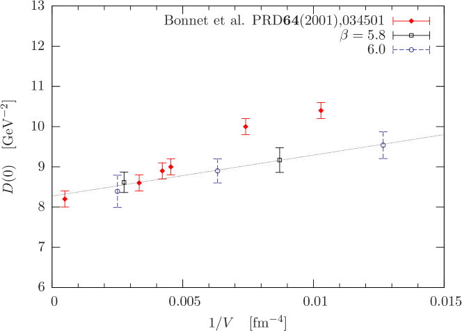
Figure 5.1: The gluon propagator at zero four-momentum, $D(0)$, plotted as a function of the inverse lattice volume. For comparison, data of the Adelaide group given in BBL⁺ [01] have been included into this figure, too. The line refers to a fit of the linear ansatz given in Eq. (5.1) to the data at $\beta=5.8$ and 6.0.

It is important to note that estimates of $\widehat{D}_{\infty}$ have to be taken with caution, because these actually do not represent the true infinite volume limit $D_{\infty}(0)$. It is also not clear whether a linear ansatz is correct BBL⁺ [01]. In this context, it is worthwhile to recall a comment already made in BBL⁺ [01] concerning the infinite volume limit. This cannot be taken such simple as outlined above. In fact, the infinite volume limit is given by

$$D_{\infty}(0)=\lim_{V\rightarrow\infty}\lim_{\genfrac{}{}{0.0pt}{1}{a\rightarrow 0}{V=\textrm{const.}}}D(0).$$ (5.2)

That is, the continuum limit (at fixed physical volume) has to be taken before the infinite volume limit. This was not done for the given estimates of $\widehat{D}_{\infty}$ and thus a complete systematic extrapolation to the infinite volume limit remains to be carried out yet BBL⁺ [01]. For this one would first need to calculate $D(0)$ using different lattice spacings $a$, while keeping the physical volume fixed. The results would then have to be extrapolated to the continuum limit. Repeating this for a variety of lattice volumes the different continuum limits obtained one could try to extrapolate to the infinite volume limit $D_{\infty}(0)$. This, of course, is the essence of the limit in Eq. (5.2).

Therefore, we think a conclusive statement of whether in Landau gauge the gluon propagator at zero momentum is finite or not cannot be made neither from our data at zero and non-zero momentum nor from the data available in the literature at present.

5.2 The Kugo-Ojima confinement parameter

In section Sec. 2.3.1 we have introduced the Kugo-Ojima confinement scenario. According to this scenario, colored asymptotic states, if any, are confined from the physical state space of QCD in covariant gauges by the quartet mechanism, if for the function $u(q^{2})\delta^{ab}\mathrel{\mathop{\mathchar 58\relax}}=u^{ab}(q^{2})$, with $u^{ab}(q^{2})$ defined in Eq. (2.17), the zero-momentum limit

$$u\mathrel{\mathop{\mathchar 58\relax}}=\lim_{q^{2}\rightarrow 0}u(q^{2})=-1$$ (5.3)

is realized. As pointed out by Kugo Kug [95], in Landau gauge this limit is connected to an infrared diverging ghost dressing function $J$. This can be easily seen from Eq. (2.18) which yields

$$\frac{1}{J(q^{2})}=1+u(q^{2})+q^{2}v(q^{2})\quad\stackrel{{\scriptstyle q^{2}\rightarrow 0}}{{\longrightarrow}}\quad 1+u(0)\;.$$

We have made an attempt to confirm the realization of the limit in Eq. (5.3) — here for lattice QCD in Landau gauge — not only by giving numerical evidence for a diverging ghost dressing function (see Sec. 4.3.2), but also by estimating the function $u(q^{2})$ for different momenta $q^{2}$ from our lattice simulations.

5.2.1 Expected infrared behavior

Before discussing numerical results it is interesting to figure out first what can be expected for the momentum dependence of $u(q^{2})$ in the infrared. In fact, due to Eq. (2.18) we know that in the limit of vanishing momenta the function $u(q^{2})$ approaches the asymptote

$$\tilde{u}(q^{2},\mu^{2})\mathrel{\mathop{\mathchar 58\relax}}=\frac{1}{J(q^{2},\mu^{2})}-1\;.$$ (5.4)

If we assume that, for example, the power law $J(q^{2},\mu^{2})\propto(q^{2}/\mu^{2})^{-\kappa}$ describes the ghost dressing function at very low momenta, then the asymptote $\tilde{u}(q^{2},\mu^{2})$, and so the function $u(q^{2},\mu^{2})$, should expose an infrared behavior as illustrated in Fig. 5.2 for different infrared exponents $\kappa$. Even if such a power law will turn out not to be appropriate for $J(q^{2},\mu^{2})$ — the results presented in Sec. 4.3.2 at least give rise to some doubt — it is commonly believed (and in agreement with our results) that the ghost dressing function diverges in the infrared; and this of course independent of the renormalization point $\mu$ chosen. Therefore, based on Eq. (2.18) the function $u(q^{2},\mu^{2})$ is expected to reach minus one and to join $\tilde{u}(q^{2},\mu^{2})$ at vanishing momentum, irrespective of the chosen $\mu^{2}$.

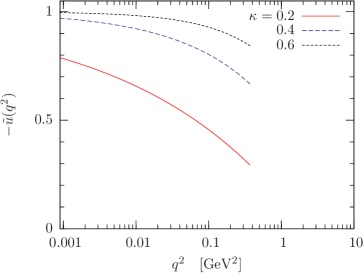
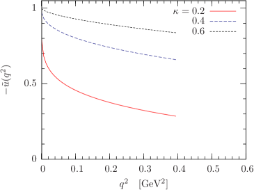
Figure 5.2: The asymptote $-\tilde{u}(q^{2},\mu^{2})$ at low momentum (see Eq. (5.4)) is illustrated in logarithmic and linear momentum scale. As ansatz for the ghost dressing function we used $J(q^{2},\mu^{2})=(q^{2}/\mu^{2})^{-\kappa}$ with $\mu=4\leavevmode\nobreak\ \textrm{GeV}$. The $\kappa$ values are 0.2, 0.4 and 0.6.

To confirm this point with numerical data, in Fig. 5.3 we show $\tilde{u}(q^{2},\mu^{2})$ as obtained from our data for the ghost dressing functions renormalized at different momenta $\mu$. In this figure we clearly see that the different curves referring to different $\mu$ approach each other slowly with decreasing momentum. With respect to Fig. 5.2 we expect that all these curves run slowly towards minus one in the zero momentum limit by definition (see Eq. (5.4)) if the ghost dressing function diverges in the infrared no matter how.

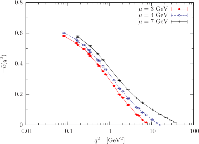
Figure 5.3: The asymptote $-\tilde{u}(q^{2},\mu^{2})$ as defined in Eq. (5.4) is shown as a function of momentum $q^{2}$. For the ghost dressing function we used our data at $\beta=5.8$ and $6.0$ renormalized either at $\mu=3$, $4$ or $7\leavevmode\nobreak\ \textrm{GeV}$. The lattice size is $32^{4}$. Lines are drawn to guide the eye.

5.2.2 Explicit lattice data for the function $\boldsymbol{u(q^{2})}$

Apart from the asymptotes $\tilde{u}$ relying solely on data for the ghost dressing functions we have also calculated on the lattice the function

$$u_{L}(q^{2})=\frac{1}{N_{c}^{2}-1}\sum_{a=1}^{N_{c}^{2}-1}u^{aa}(q^{2})$$

explicitly in terms of MC averages for $u^{ab}(q^{2})$ at different $q^{2}$ (see Eq. (3.38)). These estimates were obtained on $32^{4}$ lattice from our (quenched) gauge-fixed configurations thermalized at $\beta=5.8$ and 6.0 (see runs labeled as S-3 and S-6 in Table 4.1).

Renormalization

As for other observables the lattice data of $u_{L}(q^{2})\equiv u_{L}(q^{2},a^{2})$ have to be renormalized yet, i.e. assuming multiplicative renormalizability we have to define a factor $Z_{u}$ that relates the bare estimate $u_{L}$ to a renormalized one

$$u(q^{2},\mu^{2})=Z_{u}(\mu^{2},a^{2})\cdot u_{L}(q^{2},a^{2})\;.$$

For this we have made use again of Eq. (2.18). It relates the renormalized ghost dressing function $J(q^{2},\mu^{2})$ to the renormalized function $u(q^{2},\mu^{2})$ at finite $q^{2}$.

$$\frac{1}{J(q^{2},\mu^{2})}=1+u(q^{2},\mu^{2})+q^{2}v(q^{2})$$ (5.5)

As in Sec. 4.3.2, we have renormalized the ghost dressing function at the renormalization point $\mu=4\leavevmode\nobreak\ \textrm{GeV}$ and so with Eq. (5.5) we can renormalize $u(q^{2},\mu^{2})$ at the same point. However, the function $v(q^{2})$ (see Kug [95]) is not available to us, causing some difficulties for the determination of $Z_{u}(\mu^{2},a^{2})$.

Nevertheless, we know that for small momenta $q^{2}$ the term $q^{2}v(q^{2})$ becomes less dominant in Eq. (5.5). With the ansatz of a Taylor expansion

$$v(q^{2})=A+Bq^{2}+Cq^{4}+\ldots$$

we have made a $\chi^{2}$ fit using

$$\chi^{2}\mathrel{\mathop{\mathchar 58\relax}}=\sum_{q^{2}_{i}}\left(1+Z_{u}u_{L}(q_{i}^{2})-\frac{1}{J(q_{i}^{2},\mu^{2})}+Aq_{i}^{2}+Bq_{i}^{4}+Cq_{i}^{6}\right)^{2}$$ (5.6)

and our lattice data for $u_{L}(q^{2})$ and for $J(q^{2},\mu^{2})$ renormalized at $\mu=4\leavevmode\nobreak\ \textrm{GeV}$. By applying the momentum cut $q_{i}^{2}<2\leavevmode\nobreak\ \textrm{GeV}^{2}$ we have gained in this way $Z_{u}$ and the other parameters $A$, $B$ and $C$. The parameters are given in Table 5.1 together with a value for $\chi^{2}/\textrm{ndf}$.

Of course, the number of terms in the Taylor expansion depends on the region of momenta considered. We have found that the given order is necessary, but also sufficient in our case. Note that due to the number of parameters and the amount of data available for $q^{2}<2\leavevmode\nobreak\ \textrm{GeV}^{2}$ in the minimization process we have not distinguished between data at $\beta=5.8$ and 6.0. In general, the factor $Z_{u}(\mu^{2},a^{2})$ differs for the two $\beta$ values, but due to multiplicative renormalization there is an additional factor that relates both. From data inspection we found that we can approximate this to be one in our case.

$Z_{u}$	$A$	$B$	$C$	$\chi^{2}/\textrm{ndf}$
1.146(7)	0.22(3)	-0.21(5)	0.06(3)	0.59

Table 5.1: The parameters obtained by MINUIT after minimization of the function $\chi^{2}$ defined in Eq. (5.6). For this we used our data of $u_{L}(q^{2})$ and $J(q^{2},\mu^{2}=(4\leavevmode\nobreak\ \textrm{GeV})^{2})$ for $q^{2}<2\leavevmode\nobreak\ \textrm{GeV}^{2}$ at $\beta=5.8$ and $6.0$. The value $Z_{u}$ has been used to renormalize $u$ at $\mu=4\leavevmode\nobreak\ \textrm{GeV}$ in Fig. 5.4.

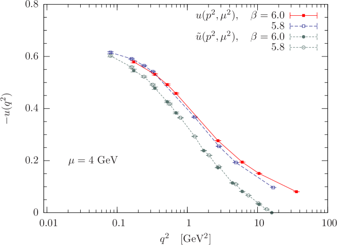
Figure 5.4: Data for the function $u(q^{2},\mu^{2})$ at $\beta=5.8$ and 6.0 are shown using full and open squares. Additionally, data of the asymptote $\tilde{u}(q^{2},\mu^{2})$ are shown at the same $\beta$ values (circles). All data refer to the same quenched configurations on a $32^{4}$ lattice and are renormalized at $\mu=4\leavevmode\nobreak\ \textrm{GeV}$ as described in the text. Lines are drawn to guide the eye.

Discussion of numerical results

In Fig. 5.4 we show data for the renormalized function $u(q^{2},\mu^{2})$ at $\beta=5.8$ and 6.0 as a function of momentum $q^{2}$. Since the ghost dressing function was renormalized at $\mu=4\leavevmode\nobreak\ \textrm{GeV}$ so was the function $u(q^{2},\mu^{2})$ mediated by the minimization process mentioned above. In this figure we also show data for the asymptote $\tilde{u}(q^{2},\mu^{2})$ renormalized at the same $\mu$. Note that only $Z_{u}$ has been of relevance for providing this figure.

We clearly see that $\tilde{u}(q^{2},\mu^{2})$ and $u(q^{2},\mu^{2})$ approach each other with decreasing momenta. Therefore, as the ghost dressing function is expected to diverge in the infrared, we expect $u(q^{2},\mu^{2})$ to approach minus one as does the asymptote $\tilde{u}(q^{2},\mu^{2})$ by definition. In Fig. 5.4 the growth of $-u(q^{2},\mu^{2})$ becomes slower as the momentum decreases, but this behavior we anticipate from our discussion above (see Fig. 5.2) concerning the infrared behavior expected for $\tilde{u}$.

Although we cannot give a reasonable extrapolation of $u(q^{2},\mu^{2})$ towards the zero momentum limit, our results for both $\tilde{u}(q^{2},\mu^{2})$ and $u(q^{2},\mu^{2})$ confirm that in the infrared the realization of the limit given in Eq. (5.3) can be studied solely in terms of the ghost propagator. As this propagator we have found to diverge stronger than $1/q^{2}$, the function $u(q^{2},\mu^{2})$ will reach minus one at zero momentum. This is because in the infrared the difference $\left|u(q^{2},\mu^{2})-\tilde{u}(q^{2},\mu^{2})\right|$ seems to vanish as we have confirmed in this study for the first time (see Fig. 5.4).

Here a remark is in order. The studies of Furui and Nakajima NF00b ; NF00a ; FN04a ; FN04b ) yield as a limit for $u(q^{2},\mu^{2})$ values ranging between $-0.7$ and $-0.83$. We cannot confirm these results in our study, because with respect to our data such limits would correspond to linear or quadratic extrapolations towards the zero momentum limit in a figure using a linear momentum scale. However, linear or quadratic extrapolations would not be valid in this context.

5.3 The gluon propagator explicitly violates reflection positivity

In this section we will show that our data for the gluon propagator presented in Sec. 4.3 show evidence for a violation of reflection positivity. To substantiate this, a subset of data obtained on our larger lattices has been selected for both the quenched and the unquenched case and then the temporal correlator $C(t,\boldsymbol{p}^{2}=0)$ of the gluon propagator has been calculated. The continuum expression of this correlator is defined in Eq. (2.23); and the lattice equivalent is given by

$$C(t)\equiv C(t,\boldsymbol{p}^{2}=0)\mathrel{\mathop{\mathchar 58\relax}}=\frac{1}{\sqrt{V}}\sum_{k_{4}=0}^{L_{T}-1}D(k_{4},\boldsymbol{0})\exp\left\{\frac{2\pi ik_{4}t}{L_{T}}\right\}$$ (5.7)

where $L_{T}$ denotes the number of lattice points in $\mu=4$ (time) direction and $D$ refers to the gluon propagator in momentum space.

Starting with the quenched gluon propagator at $\beta=6.0$, the results of the correlator are shown in Fig. 5.6 for the lattice sizes $32^{4}$ and $48^{4}$. It is obvious from this figure that the gluon propagator violates reflection positivity in a finite range of $t$. The same holds for the gluon propagator in the unquenched case as can be seen in Fig. 5.6. There we made use of our measurements of the gluon propagator on a $24^{3}\times 48$ lattice at different values of $\beta$ and $\kappa$. These values are given in Table 4.2 and the labels D-2, D-3 and D-4 refer to these.

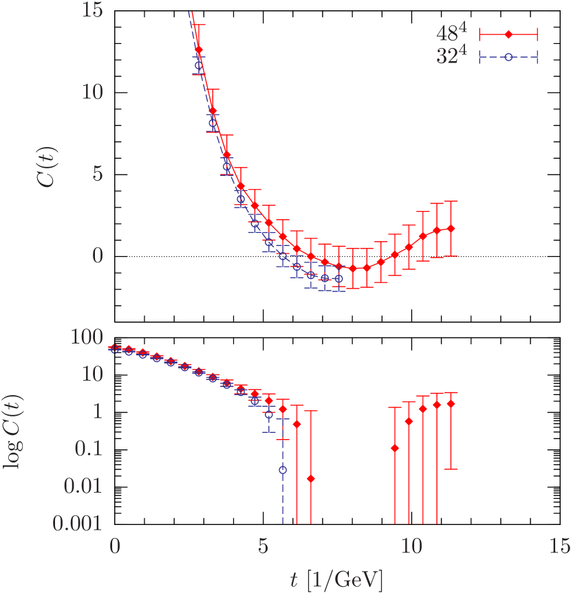
Figure 5.5: The upper panel shows the real space propagator $C(t)$ of the gluon fields in the quenched approach for different lattice sizes at $\beta=6.0$. In the lower panel the same data are shown, however, as $\log C(t)$ for $C(t)>0$.

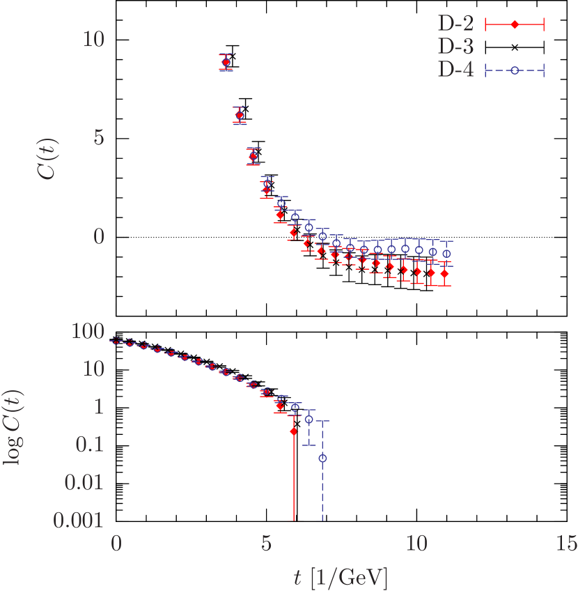
Figure 5.6: The same as in Fig. 5.6, however, for the unquenched gluon propagator on a $24^{3}\times 48$ lattice. The labels refer to the corresponding set of parameters in Table 4.2.

Following Refs. AvS [01]; A⁺ [97]; CMT [05], the statement of reflection-positivity violation can be made even more clear by considering the quantity

$$G(t,a)\mathrel{\mathop{\mathchar 58\relax}}=\frac{C(t)C(t+2a)-C^{2}(t+a)}{a^{2}}\;.$$ (5.8)

This is a discretized expression of the continuum quantity $G(t)[C(t)]^{2}$ where

$$G(t)\mathrel{\mathop{\mathchar 58\relax}}=\frac{d^{2}}{dt^{2}}\ln C(t)=\frac{C(t)C^{\prime\prime}(t)-[C^{\prime}(t)]^{2}}{[C(t)]^{2}}=\left\langle(\omega^{2}-\langle\omega\rangle^{2})\right\rangle\;.$$

Here we adopted the notation A⁺ [97]; CMT [05]

$$\langle\cdot\rangle\mathrel{\mathop{\mathchar 58\relax}}=\int(\cdot)e^{-\omega t}\rho(\omega^{2})d\omega\;.$$

If the spectral density $\rho(\omega^{2})$ is positive definite, so is $G(t)$. But if instead $G(t)$ is found to be negative then there cannot be a positive definite spectral density, which entails violation of reflection positivity. This can easily be seen in Fig. 5.8 where values of $-G(t,a=1)$ are shown for the data considered above. There $G(t,1)$ is clearly negative for all $t$ and therefore reflection positivity must be violated.

 

 

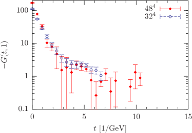
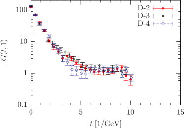
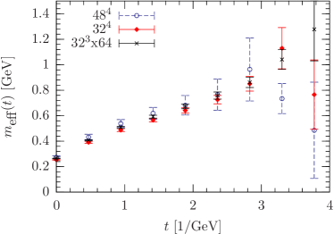
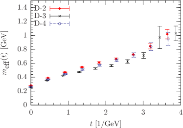
Figure 5.7: The quantity $-G(t,a)$ as defined in Eq. (5.8) is shown as a function of $t$ at $a=1$. Here we used the same quenched (left) and unquenched (right) data as in Fig. 5.6 and 5.6, respectively.

Figure 5.8: The effective gluon mass $m_{\textrm{eff}}$ of the quenched (left) and unquenched (right) gluon propagator.

Beside of $G(t)$, one usually also discusses in this context the rise of an effective gluon mass. On the lattice this can be defined as

$$m_{\textrm{eff}}(t)\mathrel{\mathop{\mathchar 58\relax}}=-\log\left\{\frac{C(t+a)}{C(t)}\right\}$$ (5.9)

where $C(t)$ again refers to the real space propagator of the gluon fields (Eq. (5.7)). Already in the first numerical study of the gluon propagator MO [87] this effective mass was observed to rise with increasing distance $t$ (see also BPS [93]; MMST [93]). In fact, the definition of $m_{\textrm{eff}}$ in Eq. (5.9) yields that CMT [05]

$$e^{m_{\textrm{eff}}(t)}-e^{m_{\textrm{eff}}(t+a)}=a^{2}G(t,a)e^{m_{\textrm{eff}}(t+a)}.$$

If reflection positivity were satisfied, then $G(t,a)$ would be positive semi-definite and therefore $m_{\textrm{eff}}(t)\geq m_{\textrm{eff}}(t+a)$. However, for the gluon propagator in Landau gauge the opposite was found. This has suggested from the beginning MO [87] that the $SU(3)$ lattice gluon propagator violates reflection positivity. With our data in Fig. 5.6 and 5.6 we show this explicitly for the quenched and unquenched $SU(3)$ gauge theory.

For the sake of completeness we have calculated the effective gluon mass also for our data. The results are plotted in Fig. 5.8 where $m_{\textrm{eff}}$ is shown as a function of $t$ for the quenched and unquenched case, respectively. The effective gluon mass is clearly rising within error bars for moderate values of $t$.

Summarizing, our study has found a clear signal for the violation of reflection positivity for both the quenched and the unquenched gluon propagator. If we consider this statement in conjunction with the results presented in the former section which support the Kugo-Ojima confinement criterion to be satisfied for lattice QCD in Landau gauge, then this supports the assumption that the transverse gluon states are confined by the quartet mechanism.

Chapter 6 Spectral properties of the Faddeev-Popov operator

[0,l,S,] pectral properties of the Landau gauge FP operator are important for understanding many aspects of QCD in Landau gauge. In this chapter we report on a study of some of these properties, restricting ourselves to the quenched approximations of lattice QCD. We shall start with a discussion of the low-lying eigenvalue distribution where the impact of the Gribov ambiguity is shown in particular. Concerning the infrared behavior of the ghost propagator discussed above here we will analyze the contribution of the different eigenvalues and eigenmodes of the FP operator to the ghost propagator at low momentum. Localization properties of the eigenmodes analyzed in addition.

6.1 Specification of lattice samples

Our investigation of the infrared behavior of ghost and gluon propagators (see Sec. 4.3) has revealed that unquenching effects are negligible within errors for the ghost propagator. We expect the same to hold for the FP operator itself. Therefore, we have analyzed its spectral properties solely in the quenched approximation of QCD.

For this analysis we have used a subset of our pure $SU(3)$ gauge configurations thermalized with the standard Wilson action at $\beta=5.8$ and $6.2$ using the lattice sizes $12^{4}$, $16^{4}$ and $24^{4}$. To study the influence of the Gribov ambiguity we followed again our fc-bc strategy introduced in Sec. 4.1.3 and have generated two ensembles of first (fc) and best (bc) gauge-fixed configurations. On those ensembles the low-lying eigenvalues $\lambda$ of the FP operator and the corresponding eigenmodes have been separately extracted. For this we used the parallelized version of the ARPACK package LMSY , PARPACK.

To be specific, the 200 lowest (non-trivial) eigenvalues and their corresponding eigenfunctions have been calculated at $\beta=6.2$ using the lattice sizes $12^{4}$ and $16^{4}$ (see Table 6.1). Due to restricted amount of computing time only 50 eigenvalues and eigenmodes have been extracted on the $24^{4}$ lattice at the same $\beta$. In addition, 90 eigenvalues have been calculated on a $24^{4}$ lattice at $\beta=5.8$ providing us with an even larger physical volume. This allows us to check whether low-lying eigenvalues are shifted towards $\lambda\to 0$ as the physical volume is increased. The eight (trivial) zero eigenvalues with the corresponding constant zero modes have always been discarded.

No.	$\beta$	lattice	# conf	# copies	# eigenvalues
F-1	5.8	$24^{4}$	25	40	90
F-2	6.2	$12^{4}$	150	20	200
F-3	6.2	$16^{4}$	100	30	200
F-4	6.2	$24^{4}$	35	30	50

Table 6.1: Statistics of data used in our analysis. The last column lists the number of eigenvalues extracted separately on fc and bc copies of $U$. At $\beta=6.2$ the corresponding eigenmodes were calculated, too. Labels given in the first row refer to the corresponding entries in Table 4.1.

6.2 The low-lying eigenvalue spectrum

We start the discussion with the two lowest (nontrivial) eigenvalues of the FP operator and then give an estimate for the density of low-lying eigenvalues.

6.2.1 The lowest and second lowest eigenvalues

The distributions of the two lowest-lying eigenvalues, $\lambda_{1}$ and $\lambda_{2}$, of the FP operator are shown for different volumes in Fig. 6.1. There $h(\lambda,\lambda+\Delta\lambda)$ represents the average number (per configuration) of eigenvalues found in the interval $[\lambda,\lambda+\Delta\lambda]$. To disentangle the distributions for the two different sets of gauge copies, open (full) bars refer to the distribution on fc (bc) gauge copies.

It is obvious from this figure that both eigenvalues, $\lambda_{1}$ and $\lambda_{2}$, are shifted to lower values as the physical volume is increased. In conjunction the spread of $\lambda$ values is shrinking. This would be even more obvious, if we had shown both distributions as functions of $\lambda$ in physical units.

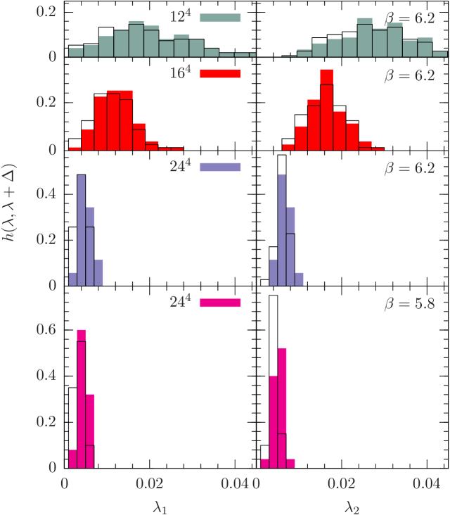
Figure 6.1: The frequency $h(\lambda)$ per configuration of the lowest (left panels) and second lowest (right panels) eigenvalue $\lambda$ of the Faddeev-Popov operator is shown. Filled boxes represent the distribution obtained on best (bc) gauge copies, while open ones represent those on first (fc) copies.

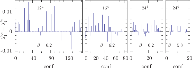
Figure 6.2: The differences $\lambda^{\texttt{bc}}_{1}-\lambda^{\texttt{fc}}_{1}$ of the lowest FP eigenvalues calculated on bc and fc representatives for each gauge configuration are shown. From left to right the lattice sizes are $12^{4}$, $16^{4}$ and $24^{4}$ at $\beta=6.2$ and $24^{4}$ at $\beta=5.8$.

It is also visible that the two low-lying eigenvalues $\lambda^{\texttt{fc}}_{i}$ ($i=1,2$) on fc gauge copies tend to be lower than those on bc copies. However, this holds only on average as can be seen from Fig. 6.2. There the differences $\lambda^{\texttt{bc}}_{1}-\lambda^{\texttt{fc}}_{1}$ of the lowest eigenvalues on fc and bc gauge copies are shown for different lattice sizes at $\beta=6.2$ and $5.8$. It is evident that there are only few cases where $\lambda^{\texttt{bc}}_{1}<\lambda^{\texttt{fc}}_{1}$, even though $F^{\texttt{bc}}\geq F^{\texttt{fc}}$ always holds for the gauge functional.

In addition we have checked how the average values $\langle\lambda\rangle$ of the respective eigenvalue distributions tends towards zero as the linear extension $aL$ of the physical volume is growing. For this the lattice spacing $a$ has been specified in physical units. As in Chapt. 4 we followed Ref. NS [02] to fix $a$. For $\beta=5.8$ and 6.2 we used $a^{-1}$=1.446 GeV and 2.914 GeV, respectively, using the Sommer scale $r_{0}=0.5$ fm.

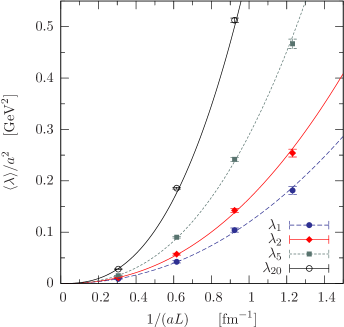
Figure 6.3: The average values $\langle\lambda_{i}\rangle/a^{2}$ (scaled to physical units) of the eigenvalues $\lambda_{i}$ $(i=1,2,5,20)$ are shown vs. the inverse of the linear lattice extension $aL$. Only eigenvalues on bc copies are shown. The lines represent fits to the data using the ansatz $a^{-2}\langle\lambda_{i}\rangle=C_{i}/(aL)^{2+\epsilon_{i}}$.

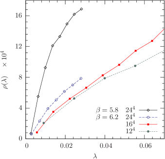
Figure 6.4: The eigenvalue density $\rho$ for bc copies as a function of $\lambda$ estimated on $12^{4}$ and $16^{4}$ lattices at $\beta=6.2$ and on a $24^{4}$ lattice for $\beta=6.2$ and $5.8$. Bin sizes have been chosen as small as possible for each lattice size. Symbols mark the middle of each bin and lines are to guide the eye.

If the low-lying eigenvalues are supplemented with physical units it turns out that the average values of their distributions tend towards zero stronger than by volume scaling proportional to $1/(aL)^{2}$. In fact, using the ansatz

$$f(aL)=\frac{C}{(aL)^{2+\varepsilon}}$$ (6.1)

to fit the data of $\langle\lambda_{i}\rangle/a^{2}$ for different $(aL)$, always a positive $\varepsilon$ is found. The parameter of these fits are given in Table 6.2 and in Fig. 6.4 we show the data and the corresponding fitting functions. There one clearly sees, the low-lying eigenvalues not only approach zero, but also become closer to each other with increasing $aL$. The latter issue has been addressed by fitting the differences $(\langle\lambda_{i+1}\rangle-\langle\lambda_{i}\rangle)/a^{2}$ of adjacent average values using the same ansatz Eq. (6.1). In Table 6.2 we give the parameter of such fits.

$a^{2}f(aL)$	$C$	$\epsilon$	$\chi^{2}/\textsc{ndf}$
$\langle\lambda_{1}\rangle$	0.120(3)	0.16(4)	0.7
$\langle\lambda_{2}\rangle$	0.165(4)	0.24(5)	1.8
$\langle\lambda_{5}\rangle$	0.290(1)	0.45(4)	3.5
$\langle\lambda_{2}\rangle-\langle\lambda_{1}\rangle$	0.045(2)	0.47(9)	0.4
$\langle\lambda_{3}\rangle-\langle\lambda_{2}\rangle$	0.051(1)	0.88(8)	0.2
$\langle\lambda_{4}\rangle-\langle\lambda_{3}\rangle$	0.033(1)	0.62(33)	2.0
$\langle\lambda_{5}\rangle-\langle\lambda_{4}\rangle$	0.037(1)	0.89(1)	0.003

Table 6.2: The parameters $C$ and $\epsilon$ from fitting either the averages $\langle\lambda_{i}\rangle/a^{2}$ or the differences of adjacent average values $\langle\lambda_{i+1}\rangle/a^{2}-\langle\lambda_{i}\rangle/a^{2}$ of the corresponding eigenvalue distributions to the ansatz $f(aL)=C_{i}/(aL)^{2+\epsilon_{i}}$.

6.2.2 An estimate for the density of low-lying eigenvalues

The eigenvalue density $\rho(\lambda)$ is of particular interest. At small $\lambda$ this quantity has been estimated here by

$$\rho(\lambda)=\frac{h(\lambda,\lambda+\Delta\lambda)}{N\Delta\lambda}\,,$$ (6.2)

i.e. the average number $h$ of eigenvalues per gauge-fixed configuration within the interval $[\lambda,\lambda+\Delta\lambda]$ divided by the bin size $\Delta\lambda$. For normalization the denominator $N=8V$ has been chosen, since the FP matrix is a $N\times N$ sparse symmetric matrix with $N$ linearly independent eigenstates. The trivial zero modes would be described by a term $8\delta(\lambda)$ in $\rho(\lambda)$ (not shown).

The estimates for the density $\rho$ are shown in Fig. 6.4 for the different volumes used. The bin sizes have been reasonably adjusted for each volume separately. In Fig. 6.4 one clearly sees the eigenvalue density close to $\lambda=0$ becomes steeper as a function of $\lambda$ as the physical volume becomes larger. It is remarkable that the increase going from $\beta=6.2$ to $\beta=5.8$ on a $24^{4}$ lattice is larger than going from $12^{4}$ to $24^{4}$ at $\beta=6.2$ fixed, although in both cases the physical volume is increased by a factor of about 16.

6.3 Eigenmode expansion of the ghost propagator

Along with the calculation of the low-lying eigenvalues, the corresponding eigenvectors $\boldsymbol{\phi}(x)$ have been determined as well. These are of particular importance for the infrared behavior of the ghost propagator as it becomes clear from Eq. (3.37). In fact, if all eigenvalues $\lambda_{i}$ of the FP operator and the corresponding eigenvectors $\boldsymbol{\Phi}_{i}(k)$ in momentum space were available the ghost propagator could be constructed out of them according to Eq. (3.37) and (3.36). Unfortunately, their determination for each configuration is numerically too demanding.

However, restricting the sum in Eq. (3.37) to the $n$ lowest eigenvalues and eigenvectors ($n\ll N=8V-8$), we can figure out to what extent these modes, i.e. the corresponding estimator Eq. (3.36) and (3.37)

$$G_{n}(q^{2}(k))=\langle G(k|n)\rangle_{\textrm{MC}}$$

where

$$G(k|n)=\frac{1}{8}\leavevmode\nobreak\ \sum_{i=1}^{n}\frac{1}{\lambda_{i}}\,\boldsymbol{\Phi}_{i}(k)\cdot\boldsymbol{\Phi}_{i}(-k)$$

saturates the full ghost propagator $G(q^{2})$. The latter is obtained, of course, independently for a set of momenta by inverting the FP matrix on a set of plane waves. See Sec. 4.3.2 for the corresponding data of $G(q^{2})$.

The degree of saturation is shown in Fig. 6.5 for the lowest $q^{2}_{1}$ and the second lowest momentum $q^{2}_{2}$ available on different lattice sizes for $\beta=6.2$. There the values of $G_{n}(q^{2})$ have been presented relative to the values for the full propagator $G(q^{2})$ in order to assess the saturation for different volumes. Since $\boldsymbol{\Phi}_{i}(k)$ has been obtained by a fast Fourier transformation of the eigenvector $\boldsymbol{\phi}_{i}(x)$, all lattice momenta $k$ are available. Thus $G_{n}(q^{2})$ refers to the average over all $k$ giving raise to the same momentum $q^{2}$. The full propagator values $G(q^{2})$ at $q^{2}_{1}(k)$ and $q^{2}_{2}(k)$, however, refer to the averages over lattice momenta $k=([1,0],0,0)$ and to $k=(1,1,0,0)$, respectively.

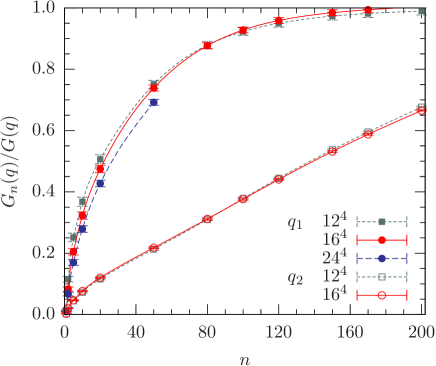
Figure 6.5: The ratio of the truncated ghost propagator $G_{n}(q^{2})$ (in terms of the $n$ lowest FP eigenmodes and eigenvalues) to the full estimate $G(q^{2})$ (taken from SIMPS05d ) shown as a function of $n$ for the lowest ($q^{2}_{1}$) and second lowest ($q^{2}_{2}$) momentum. The inverse coupling is $\beta=6.2$ and the lattice size ranges from $12^{4}$ to $24^{4}$. All data refer to bc copies.

Let us consider first the lowest momentum $q^{2}_{1}$. We observe from Fig. 6.5 that the approach to convergence differs, albeit slightly, for the three different lattice sizes. The relative deficit for $n<50$ rises with the lattice volume. For $n>100$ the rate on a $16^{4}$ lattice is even a bit larger than that on a $12^{4}$ lattice. We could not afford to get data for $n>50$ on the $24^{4}$ lattice. However, for the $12^{4}$ and $16^{4}$ lattices the rates of convergence are about the same. For example, taking only 20 eigenmodes one is definitely far from saturation (by about 50%) whereas 150 to 200 eigenmodes are sufficient to reproduce the ghost propagator within a few percent. In other words, the ghost propagator at lowest momentum on a $12^{4}$ ($16^{4}$) lattice is formed by the lowest 0.12% (0.03%) of the eigenvalues and eigenfunctions of the FP operator.

For the second lowest momentum $q^{2}_{2}$ the contribution of even 200 eigenmodes is far from being sufficient to approximate the propagator.

6.4 The problem of exceptional configurations

We turn now to a peculiarity of the ghost propagator at larger $\beta$ of which has been reported already in SIMPS05d ; SIMP [06]. It was also seen in an earlier $SU(2)$ study BIMMP [04]. While inspecting our data we found, though rarely, that there are exceptionally large values in the Monte Carlo (MC) time histories of the ghost propagator at lowest momentum.

In Fig. 6.6 such time histories are shown of the ghost propagator on fc and bc gauge copies for the two smallest momentum realizations $k=(1,0,0,0)$ and $k=(0,1,0,0)$. From left to right the panels are ordered in ascending order with the (physical) lattice sizes $12^{4}$, $16^{4}$ and $24^{4}$ at $\beta=6.2$ and $24^{4}$ at $\beta=5.8$.

 

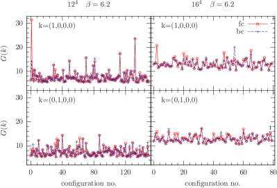
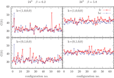
Figure 6.6: The MC time histories of the ghost propagator calculated on first (fc) and best (bc) gauge copies on a $12^{4}$, $16^{4}$ and $24^{4}$ lattice at $\beta=6.2$ and $24^{4}$ lattice at $\beta=5.8$. From left to right the corresponding runs listed in Table 6.1 and Table 4.1 are F-2, F-3, F-4/S-9 and F-1/S-2. The upper and lower panels show data for the lowest momentum realization $k=(1,0,0,0)$ and $k=(0,1,0,0)$, respectively.

As can be seen from this figure in the majority extreme spikes are reduced (or even not seen) when the ghost propagator could be afforded to be measured on a better gauge copy (bc) for a particular configuration. Furthermore, it is obvious that the exceptionality of a given gauge copy is exhibited not simultaneously for all different realizations of the lowest momentum. Consequently, to reduce the impact of such large values on the evaluation of a statistical average for the ghost propagator one should average, if possible, over all momentum realizations giving rise to the same momentum $q^{2}$.

We have tried to find a correlation of such outliers in the history of the ghost propagator with other quantities measured in our simulations. For example we have checked whether there is a correlation between the values of the ghost propagator $G(k)$ as they appear in Fig. 6.6 and the lowest eigenvalue $\lambda_{1}$ of the FP operator.

In Fig. 6.8 we show such correlation in a scatter plot for different lattice sizes at $\beta=5.8$ and $6.2$. There each entry corresponds to a pair $[\lambda_{1},G(k)]$ measured on a given gauge copy of our sets of fc and bc copies. It is visible in this figure, gauge copies giving rise to an extremely large MC value for the ghost propagator are those with very low values for $\lambda_{1}$. This holds for the $12^{4}$ and $16^{4}$ lattice. However, a very low eigenvalue is not sufficient to obtain large MC values for $G(k)$ as can be seen in the same figure. It is possible, of course, that such gauge copies with extremely small eigenvalues would turn out to be exceptional for another realization of lowest momentum $q^{2}(k)$ than those two we have used. This might explain why some configurations with extremely small lowest eigenvalues were not found to be exceptional with respect to the ghost propagator at $k=(1,0,0,0)$ and $k=(0,1,0,0)$.

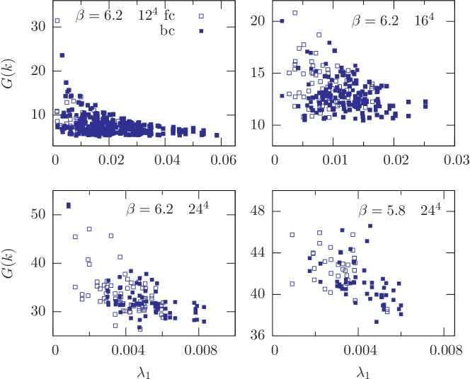
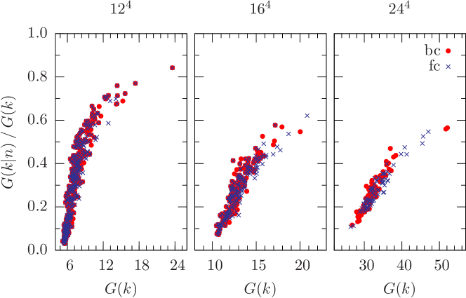
Figure 6.7: Scatter plots of MC time history values of the ghost propagator $G(k)$ at $k=([1,0],0,0)$ vs. the lowest FP eigenvalue $\lambda_{1}$ are shown. The upper panels show data at $\beta=6.2$ on a $12^{4}$ (left) and $16^{4}$ (right) lattice, the lower ones on a $24^{4}$ lattice at $\beta=6.2$ (left) and $\beta=5.8$ (right). Open symbols refer to fc gauge copies and filled symbols to bc copies.

Figure 6.8: Scatter plot of the relative contribution of the truncated sums $G(k|n)$ over eigenmodes (see Eq. (3.37)) to the full ghost propagator values $G(k)$ versus $G(k)$ for lattice momenta $k=(1,0,0,0)$ and $k=(0,1,0,0)$. From left to right the lattice sizes are $12^{4}$, $16^{4}$ and $24^{4}$ all for $\beta=6.2$. Data for fc and bc gauge copies have been plotted separately.

In the light of Eq. (3.37) it is not adequate to concentrate just on the lowest eigenvalues. Instead, one can monitor the contribution of a certain number of eigenvalues $\lambda_{i}$ and eigenmodes $\boldsymbol{\Phi}_{i}(k)$ to the ghost propagator at some momentum in question. Therefore, we have compared the truncated sums $G(k|n)$ according to Eq. (3.37) with the MC history values of the full ghost propagator $G$. In fact, we show in the scatter plots in Fig. 6.8 the ratios $G(k|n)/G(k)$ versus $G(k)$ for $n=10$ and for various lattice sizes.

Obviously there is a strong correlation between the chosen group of low-lying modes and the MC time history values of the full ghost propagator. Indeed, if we consider values $G(k)>15$ to be exceptional in the left-most panel ($12^{4}$ lattice) we find that the contribution of the 10 lowest modes amounts to more than 75% of the actual value of the ghost propagator. On the opposite, for low $G(k)$ values the main contributions come necessarily from the higher eigenmodes, while the 10 lowest modes contribute a minor part only. A similar but less dominant contribution of the 10 lowest modes is found for the time histories produced on larger lattices ($16^{4}$, $24^{4}$).

6.5 Localization properties of low-lying eigenvectors

In recent years a good deal of attention has been directed to the localization properties of various operators (Dirac operator, covariant Laplacian) in the hope to understand more about confinement beyond heavy quark probes. The first quantity of interest is the inverse participation ratio (IPR). Given an eigenvector $\boldsymbol{\phi}(x)$ the IPR is defined as

$$\mbox{{IPR}}=V\sum_{x}|\boldsymbol{\phi}(x)|^{4}\qquad\textrm{with}\;V=L^{4}.$$

Although a direct physical meaning for this quantity is lacking yet, it is a measure for the localization of an eigenvector. It enables us to distinguish between eigenmodes with approximately uniformly distributed modulus squared $|\boldsymbol{\phi}(x)|^{2}$ ($\mbox{{IPR}}\approx 1\ldots 2$) and more specific ones with a small number of sites $x$ having large intensity $|\boldsymbol{\phi}(x)|^{2}$ ($\mbox{{IPR}}\sim\textrm{O}(100)$) where they might be pinned down by special local gauge field excitations. Note, the eight (trivial) zero modes ($\lambda=0$) of the FP operator are constant and have $\mbox{{IPR}}{}=1$.

In Fig. 6.9 the relative distribution $h$ of IPR values per gauge-fixed configuration are shown, separately for certain groups of eigenstates. Again open (full) histogram bars refer to the distribution on fc (bc) gauge copies. From this figure we learn that the majority of eigenvectors of the Faddeev-Popov operator is not localized independent of the choice of gauge copies. In any case, the rare cases of large IPR values have been found among the 10 lowest non-zero eigenmodes. This becomes more likely as the physical volume is increased. So far we have no physical interpretation what causes the stronger localization in these rare cases.

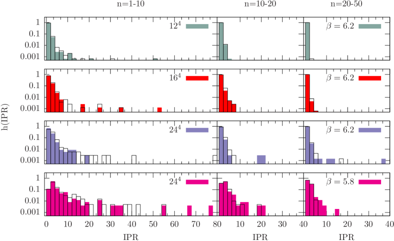
Figure 6.9: The relative distribution $h$ of IPR values of the 10 (left), the 10 to 20 (middle) and the 20 to 50 (right) lowest eigenmodes are shown. Note there is a logarithmic scale for $h(\mbox{{IPR}}{})$. Each row corresponds to one pair of $\beta$ and lattice size. Filled boxes refer to distributions on bc gauge copies, while open ones correspond to fc copies.

[0,l,I,] n this study we have focused on the infrared properties of $SU(3)$ gluodynamics in Landau gauge using the framework of lattice QCD. We have tried to cover as much as possible the different aspects relevant within this context and to verify several assumptions made in recent years. In doing so, we hope to have provided a consistent analysis of several issues that have an effect on the infrared behavior of gluon and ghost propagators, and that, in turn, the behavior we have found satisfies necessary criteria for confinement which apply to QCD in Landau gauge.

For this study we used the Wilson formulation of lattice QCD with and without dynamical clover-improved Wilson fermions. The gauge group was fixed to $SU(3)$. The quenched gauge configurations were generated at the three values $\beta=5.8$, 6.0 and 6.2 using a variety of different symmetric and asymmetric lattice geometries. In the symmetric case we used the lattice sizes $12^{4}$, $16^{4}$, $24^{4}$, $32^{4}$ and $48^{4}$, whereas the asymmetric lattices were chosen to be of size $24^{3}\times 48$, $32^{3}\times 64$, $16^{3}\times 128$ and $24^{3}\times 128$. To study unquenching effects we have analyzed gauge configurations provided to us by the QCDSF collaboration. These configurations were thermalized on a $24^{3}\times 48$ lattice in the presence of two flavors of clover-improved Wilson fermions using three different pairs of $\beta$ and $\kappa$. The corresponding lattice spacings are comparable to that at $\beta=6.0$ in the quenched case.

Both the quenched and unquenched configurations were transformed such that they satisfy the lattice Landau gauge condition. For gauge-fixing we used either over–relaxation or Fourier–accelerated gauge-fixing. A subset of our quenched configurations was gauge-fixed even more than once, always starting from a different random gauge copy of the initial (unfixed) configuration. This has allowed us to examine how the Gribov ambiguity affects the gluon and ghost propagators and the eigenvalue spectrum of the FP operator.

In the following we give a summary of our results presented in previous chapters. Then we draw our conclusions and give recommendations for future studies.

The influence of the Gribov ambiguity

We have demonstrated that the presence of Gribov copies systematically affects the ghost propagator at low momentum, whereas for the gluon propagator such an effect stays within error bars (see also SIMPS05d ). To be specific: Measuring the ghost propagator and ignoring the Gribov ambiguity, the ghost propagator near the momentum $q^{2}=0.2\leavevmode\nobreak\ \!\textrm{GeV}^{2}$ ($1\leavevmode\nobreak\ \!\textrm{GeV}^{2}$) turns out to be overestimated by about 5% (2%) compared to an estimate obtained on a ensemble of best gauge copies. As best we have considered that gauge-fixed copy which gave rise to the largest gauge functional value for a particular gauge configuration. Our results corroborate previous findings for the $SU(2)$ gluon and ghost propagators Cuc [97]; BIMMP [04]; NF04a , but cast doubt on those for the $SU(3)$ gluon propagator ($\beta=5.8$, $12^{4}$ lattice) in SO [04].

Additionally, our data are in favor of the picture promoted in Zwa [04]. According to this, continuum vacuum expectation values of correlation functions obtained from a functional integration over the fundamental modular region $\Lambda$ are equal to those over the Gribov region $\Omega$. Gribov copies inside $\Omega$ should not affect expectation values in the continuum, because functional integrals are dominated by the common boundary of $\Lambda$ and $\Omega$. We have found some numerical evidence that the influence of Gribov copies on the ghost propagator decreases at the same (physical) momentum if the physical volume is enlarged. Note that very recently BBMPM [05] similar indications have been found for the $SU(2)$ gauge group taking non-periodic $Z(2)$ transformations into account. In order to eliminate the last doubts, a future study should continue and follow our fc-bc strategy (explained in the text) on lattice sizes larger than $24^{4}$.

To make the study of the Gribov-copy dependence more complete, we have also shown that the Gribov ambiguity is reflected in the low-lying eigenvalue spectrum of the FP operator. We have found that, on average, the low-lying eigenvalues extracted on bc gauge copies are larger than those on fc copies. Thus better gauge-fixing (in terms of the gauge functional) has the tendency to keep gauge-fixed configurations slightly away from the Gribov horizon.

Other systematic effects on the propagators

Using different lattices sizes at three different $\beta$ values, we have tried to analyze the systematic effects on the gluon and ghost propagators of changing either the lattice spacing $a$ or the physical volume $V$. We have found that for both, the gluon and ghost dressing functions, finite volume effects are clearly visible at volumes smaller than $(2.2\leavevmode\nobreak\ \textrm{fm})^{4}$, which corresponds to a $16^{4}$ lattice at $\beta=5.8$. The effect grows with decreasing momentum or decreasing lattice size. At larger volumes, however, the data for $q>1\leavevmode\nobreak\ \textrm{GeV}$ coincide within errors for the different lattice sizes. For $q<1\leavevmode\nobreak\ \textrm{GeV}$ we have found only small finite volume effects for both dressing functions at the lowest momentum. This is based on data obtained on the lattice sizes $24^{4}$, $32^{4}$ and $48^{4}$ using $\beta=5.8$ and 6.0. Concerning discretization effects our study is only partial and limited to a region of intermediate momenta. In any case, fixing the physical volume to $V\approx(2.2\leavevmode\nobreak\ \textrm{fm})^{4}$ we have found that the gluon dressing function at constant physical momentum increases with decreasing the lattice spacing. A similar effect (beyond error bars) is not observable for the ghost dressing function.

We have combined this investigation of lattice artifacts with an analysis of effects caused by asymmetric lattice geometries. We could demonstrate that the more asymmetric the lattice size has been chosen, the larger are the systematic errors induced by that. In fact, data obtained for the ghost (gluon) propagator on asymmetric lattices are less enhanced (suppressed) than those obtained on symmetric lattices geometries. The same effects have been reported recently for the gluon propagator in three-dimensional pure $SU(2)$ gauge theory CM [06]. Therefore, extractions of an infrared exponent for the gluon propagator using only on-axis momenta on asymmetric lattices SO05b ; SO05a (without adapting the lattice spacing in the different directions to compensate this) should be taken with caution.

Infrared behavior of gluon and ghost propagators

Studying the momentum dependence of the gluon and ghost dressing functions, we have applied cuts on our data, namely the cylinder and the cone cut LSWP [99]. They have much reduced the lattice artifacts mentioned above. In fact, our data for the renormalized dressing functions surviving these cuts lie on smooth curves if considered as functions of the momentum.

We have compared these renormalized data with recent solutions of truncated system of DSEs for the gluon and ghost propagators and have tried to extract the infrared exponents, $\kappa_{D}$ and $\kappa_{G}$, for the gluon and ghost dressing functions, respectively. From fits with the corresponding power laws to our data we cannot confirm the relation $\kappa_{G}=2\kappa_{D}$ as expected from DSE studies in the continuum vSAH [97]; vSHA [98]. Also, both exponents are found to be significantly lower than expected in LvS [02]; Zwa [02]. Such a conclusion was also drawn in other lattice studies B⁺05b ; B⁺06a ; FN04b .

Moreover, our fits suggest that power-behaved gluon and ghost propagators are not the best description of the momentum dependence of our data, at least in the region of lower momenta considered here. The data for the ghost propagator seem to depend logarithmically on the momenta in this region. This observation has been confirmed very recently in B⁺06a , even though in this reference also arguments for an infrared finite ghost dressing function have been put forward.

Studying unquenching effects on the gluon and ghost propagators we have found that these effects are small for the ghost propagator, but are clearly visible for the gluon propagator at intermediate momenta. Concerning the infrared limit of both propagators, the influence of two fermion flavors seems to become less towards lower momenta. This all agrees with the findings in DSE studies (e.g. FA [03]; FAC⁺ [06]).

From our data, we cannot judge without doubt on the existence of an infrared vanishing gluon propagator.

The running coupling constant and the ghost-gluon vertex

In connection with the infrared behavior of the gluon and ghost dressing functions, we have determined the running coupling constant based on the ghost-gluon vertex. This coupling constant is found to match the RG-invariant two-loop expression considering data at large momenta. However, for $q^{2}<0.4\leavevmode\nobreak\ \textrm{GeV}^{2}$ the running coupling constant decreases with decreasing momentum. The same is observed considering data for the unquenched case. Also an influence of Gribov copies cannot be made responsible for this. Therefore, we cannot confirm an infrared fixed point for this coupling constant as it has been proposed in DSE studies vSAH [97]; vSHA [98] (see also AFLE [05]). This reflects once more the different infrared exponents we have found for the gluon and ghost propagators.

In any case, our data are in qualitative agreement with recent studies of DSEs on a torus FAR [02]; FA [02]; FGA [06]; FP [06]. There a similar behavior for the gluon and ghost propagators and for the running coupling constant at low momentum has been presented. Also other lattice studies agree with our results for this coupling constant FN04a ; FN04b ; B⁺05b .

In order to verify that the assumption of a bare ghost-gluon vertex is valid beyond perturbation theory, we have calculated the corresponding renormalization constant $\widetilde{Z}_{1}$ using a MOM scheme with zero gluon momentum. Our data show that in this scheme $\widetilde{Z}_{1}$ is approximately equal to one within error bars for all momenta considered here. Only a slight deviation is visible in the interval $0.3\leavevmode\nobreak\ \textrm{GeV}^{2}\leq q^{2}\leq 2\leavevmode\nobreak\ \textrm{GeV}^{2}$. Unquenching effects are not resolvable. We thus agree with a recent DSE study SMWA [05] where a semiperturbative calculation of $\widetilde{Z}_{1}$ has been presented using a MOM scheme with asymmetric (the same as used by us) and symmetric subtraction points. Furthermore, our results are in full agreement with those presented in CMM [04] for the case of $SU(2)$. It is worthwhile to continue the lattice calculation of $\widetilde{Z}_{1}$ using other renormalization schemes, for example with a symmetric subtraction point.

Together with our data for the running coupling constant we can thus confirm that the product in Eq. (2.10) is renormalization-group invariant in the particular MOM scheme considered here and defines a nonperturbative running coupling constant which, as shown here, decreases monotonously with decreasing momentum $q^{2}<0.4\leavevmode\nobreak\ \textrm{GeV}^{2}$.

Results on the confinement criteria

In addition we have presented results which support the Kugo–Ojima confinement scenario KO [79] to be realized for lattice QCD in Landau gauge. To confirm this, one has to show that the function $u^{ab}(q^{2})=u(q^{2})\delta^{ab}$ defined via the Green’s function in Eq. (2.17) Kug [95]; AvS [01] has the zero-momentum limit: $u(0)=-1$. Alternatively, if this limit is realized then the (renormalized) ghost dressing function $J(q^{2})$ must diverge in the same limit. This is because at zero momentum it holds that $1+u(0)=1/J(0)$ Kug [95].

In this thesis we have shown that the ghost dressing function seems to diverge at zero momentum which is in favor of the Kugo–Ojima confinement scenario and also satisfies the Gribov-Zwanziger horizon condition Gri [78]; Zwa [93, 02]. Moreover, we have measured the function $u(q^{2})$ at different momenta $q^{2}$. To our knowledge a direct calculation of $u(q^{2})$ has never been done before. Conclusions in other studies FN04a ; FN04b ; WA [01]; AvSW [01] were drawn on results obtained for the ghost dressing functions only. For the renormalization of $u(q^{2})$ we have developed a new ansatz using a minimization process (see Sec. 5.2.2 for details). Our renormalized data for both the ghost dressing function and the function $u(q^{2})$ are consistent with $u(q^{2})-J^{-1}(q^{2})$ approaching minus one in the limit of vanishing momenta, even though this convergence is very slow. Therefore, as the ghost dressing function diverges we expect $u(q^{2})$ to reach minus one. Hence the Kugo-Ojima confinement criterion is realized.

Based on our data obtained on larger lattice sizes we are also in the fortunate position to present numerical evidence that not only the quenched but also the unquenched $SU(3)$ gluon propagator in Landau gauge violates reflection positivity explicitly. Thus, on one hand, we agree with other lattice studies for quenched $SU(3)$ MO [87]; BPS [93]; MMST [93]; FN04b and for three-dimensional $SU(2)$ CMT [05] gauge theory. On the other hand, we confirm presently available solutions to the corresponding DSE of the gluon propagator ADFM [04], even though our data suggest a different infrared exponent for the gluon propagator.

Since reflection positivity is violated by the gluon propagator and the Kugo–Ojima confinement criterion seems to be satisfied, we agree with the conjecture that transverse gluon states are confined by the quartet mechanism KO [79].

Spectral properties of the FP operator

We have also investigated the spectral properties of the FP operator and their relation to the ghost propagator in $SU(3)$ Landau gauge SIMP [06]. As expected from Ref. Zwa [04] we have found that the low-lying eigenvalues are shifted towards $\lambda=0$ and the eigenvalue density $\rho(\lambda)$ becomes a steeper rising function as the volume is increased.

On average, the corresponding FP eigenmodes are not localized, however, a few large IPR values have been seen among the lowest eigenmodes.

We could demonstrate that the ghost propagator at low momentum is dominated by the low-lying eigenvalues and eigenmodes of the FP operator. For example, the value of the ghost propagator at lowest momentum (on a $12^{4}$ lattice at $\beta=6.2$) can be estimated using a number of 200 low-lying eigenvalues and eigenmodes of the FP operator. In other words, a fraction of about 0.12% of the whole spectrum is sufficient to reconstruct the asymptotic result. For larger volumes the number of necessary eigenmodes seems to be somewhat larger. Also for the next higher momentum, saturation needs a much bigger part of the low-lying spectrum.

We hope to have presented a careful numerical study of different aspects of $SU(3)$ Landau gauge gluodynamics, a subject which has been the focus of much attention in recent years. We have concentrated on the low momentum region and have clarified the influence of different systematic effects on the infrared behavior of gluon and ghost propagators in Landau gauge. We have shown that the momentum dependence of both propagators is consistent with different criteria for confinement. Considering also our results for the running coupling constant and for the ghost-gluon vertex we agree with the findings of other lattice studies and of DSE studies on a torus. However, there is some disagreement with DSE studies in the continuum. At present there seems to be no solution of this puzzle.

We think, it is interesting to look in a future study also at the momentum dependence of other vertex functions and of the quark propagator in Landau gauge. In particular, for clover-improved Wilson fermions this has not been done before. It is also worthwhile to perform a similar study using another gauge condition, for example, the Coulomb gauge. Such investigations might provide further valuable information towards a full understanding of nonperturbative QCD (see e.g. Zwa [98]; CZ [02]; Zwa03a ; GO [03]).

In the same way, the larger momentum region should be investigated further. Note that our study has focused only on the infrared momentum region. Since computing time was restricted, the amount of data for the ghost propagator and for the running coupling constant in the ultraviolet momentum region is not as large as in the low momentum region. It is worthwhile, however, to continue and to perform additional measurements at larger momenta considering different loop-expansions of the corresponding asymptotic form. In particular, an investigation of nonperturbative power corrections to the ghost and gluon propagators in Landau gauge (see e.g. B⁺00b ; B⁺00a ; B⁺ [01]; B⁺06b ) due to non-zero values of QCD condensates could be an interesting topic in future lattice studies.

Appendix A Some details on algorithms and performance

[0,l,W,] e list algorithms and numerical libraries used in this study for the different purposes and we give references for further details. Then we report on some experiences we gained with gauge-fixing. In particular, we compare the performance of over-relaxation and Fourier-accelerated gauge-fixing. After this, we analyze gauge functional values obtained by following our fc-bc strategy and demonstrate that the final ranking of functional values is already visible at an intermediate iteration step. We show that the inversion of the FP matrix can be accelerated by using a pre-conditioned conjugate gradient algorithm.

A.1 A note on the algorithms used

For the generation of our quenched configurations we employed the hybrid over-relaxation algorithm. It has become standard for the simulation of pure gauge theory and is a combination of several, say $N_{ov}$, micro-canonical over-relaxation steps BW [87]; Cre [87] and one heatbath FH [84]; KP [85] step. In both steps a decomposition of $SU(3)$ link variables into $SU(2)$ matrices, as proposed by Cabbibo and Marinari CM [82], was applied. We have always used $N_{ov}=4$. Further details on these algorithms can be found, for examples, in the PhD theses Kne [99]; Geh [02].

All sets of our unquenched $SU(3)$ gauge configurations were provided to us through the QCDSF collaboration which generated them using the hybrid Monte Carlo algorithm DKPR [87]; GLT⁺ [87] with even-odd preconditioning G⁺ [89].

Both the quenched and unquenched configurations were transformed such that they satisfy the lattice Landau gauge condition (see Eq. (4.1)). For gauge-fixing we have employed two popular algorithms: over-relaxation (RLX) MO90a and Fourier–accelerated gauge-fixing (FAG) D⁺ [88]. For Fourier–accelerated gauge-fixing we used the implementation as introduced in D⁺ [88]. For future studies, however, we recommend to use the multigrid implementation of FAG as proposed in CM [98]. This implementation is better suited for a parallel computing environment with distributed memory (see App. A.2.1).

Fourier transforms, for example of the gluon fields, were calculated using an algorithm that performs a Fast-Fourier transformation (FFT). For all FFTs, we have employed the FFTW-library FJ [98]. We can recommend this library (see also online: http://www.fftw.org).

For observables which involve the inverse of the FP operator we applied the pre-conditioned conjugate gradient algorithm to solve the corresponding linear systems. As pre-conditioning matrix we used the inverse Laplacian operator $\Delta^{-1}$ with diagonal color substructure. This significantly has reduced the amount of computing time as it is discussed in more detail in App. A.3.

The eigenvalues and eigenmodes of the FP operator were calculated using the ARPACK package, PARPACK LMSY . For minimization of $\chi^{2}$ functions we used the new C++ implementation of the library MINUIT JW [04]. We can recommend both libraries too.

A.2 Experience report on lattice Landau gauge fixing

In this section we report on some experiences we made with gauge-fixing. Since efficiency of gauge-fixing algorithms is an important issue in studying gauge-dependent quantities, this report might help in future studies.

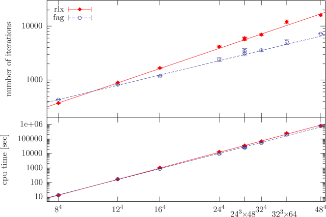
Figure A.1: The average number of iterations for both gauge-fixing using over-relaxation (rlx) and gauge-fixing using the Fourier-accelerated method (fag) is shown in the upper panel. The lower panel shows the corresponding CPU time in seconds (sum over all processors).

A.2.1 Over-relaxation versus Fourier–accelerated gauge-fixing

For the purpose of this study we have employed two different algorithms for fixing thermalized gauge configurations to Landau gauge. These are over-relaxation (RLX) MO90a and Fourier–accelerated gauge-fixing (FAG) D⁺ [88]. Both algorithms are commonly used in the lattice community, but usually either of them is chosen. The reason why we used two is simple: Initially, we had started with over-relaxation, but later we checked whether computing time can be saved using FAG instead. Now this puts us in the fortunate position to provide an explicit cross-check on the performance of both algorithms. This might be interesting for future studies, in particular when writing applications for computing time.

Even though both algorithms are quite different, they are both iterative in nature. After each iteration-cycle the functional $F_{U}[g]$ (Eq. (3.14)) is increased a bit until a (local) maximum is reached. As stopping criterion not the functional itself, but the violation of transversality (see Eq. (3.15)) is used. In our implementation the iteration process stopped as soon as $\Theta<10^{-14}$ with

$$\Theta\mathrel{\mathop{\mathchar 58\relax}}=\max_{x}\operatorname{\mathfrak{Re}}\operatorname{Tr}\left[(\nabla_{\mu}{}^{g}\!\!A_{x,\mu})(\nabla_{\mu}{}^{g}\!\!A_{x,\mu})^{\dagger}\right]$$ (A.1)

was fulfilled at each lattice site $x$. The number of necessary iterations depends on the lattice sizes, but usually it also varies quite strongly for different configurations using the same lattice size. To get an impression about these variations have a look at Fig. A.2. There $\Theta$ is shown versus the numbers of iterations for two different random gauge copies of the same gauge configuration.

In any case, the mean iteration number $N_{\textrm{iter}}$ and the mean iteration time $T_{\textrm{iter}}$ (until the final precision is reached) scale with the lattice size $V=L_{S}^{3}\times L_{T}$ according to

$$N_{\textrm{iter}}(V;a,b) = a\cdot V^{b}\;,$$ (A.2a)

$$T_{\textrm{iter}}(V;c,d) = c\cdot V^{d}\;.$$ (A.2b)

$L_{S}$ and $L_{T}$ denote the number of lattice points in spatial and temporal direction, respectively. That this scaling holds for both algorithms can be seen in Fig. A.1. There in the upper (lower) panel we show $N_{\textrm{iter}}$ ($T_{\textrm{iter}}$) as a function of the lattice size. The parameters from fits of the Ansätze in Eq. (A.2) to the data are given in Table A.1. Obviously, FAG performs better on larger lattice sizes than RLX.

	$N_{\textrm{iter}}$			$T_{\textrm{iter}}$
	a	b	$\chi^{2}/ndf$	c	d	$\chi^{2}/ndf$
rlx	4.5(2)	0.53(1)	1.6	$3.2(4)\cdot 10^{-5}$	1.55(1)	5.6
fag	19(2)	0.38(1)	3.0	$5.0(9)\cdot 10^{-5}$	1.51(2)	8.1

Table A.1: The parameters of the functions $\texttt{iter}(V;a,b)$ and $\texttt{cpu}(V;c,d)$ fitted to the average number of iterations and average CPU time, respectively.

The reason why in our implementation the actual amount of computing time for FAG is comparable to that of RLX is just because we have performed two Fast-Fourier transformations (FFTs) in each iteration cycle of FAG. Of course, in a parallel computing environment with distributed memory FFT routines usually do not scale well if the number of processors in increased. Therefore, for future studies we rather recommend to use the multigrid implementation of FAG as proposed by Cucchieri and Mendes CM [98].

A.2.2 A way to preselect best gauge copies

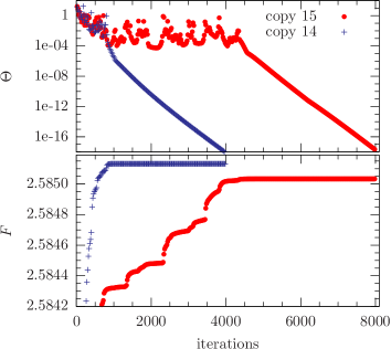
Figure A.2: The values of $F$ and $\Theta$ (see Eq. (3.14) and (A.1)) and are shown as functions of the iteration number for two sample gauge copies of the same configurations ($\beta=6.0,24^{4}$).

We have seen above that fixing gauge configurations to Landau gauge might become a CPU time intensive task on large lattices. This was even more intensive for us when we followed our fc-bc-strategy (see Sec. 4.1.3). For this, several random gauge copies for each gauge configuration $U$ were gauge-fixed. Then we have selected the first gauge copy and that with the largest (final) functional value (Eq. (3.14)) to study the influence of Gribov copies on different observables. Obviously, it would be quite helpful if the final ranking of functional values were known, without actually doing all the necessary iterations.

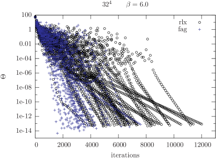
Figure A.3: The local maximum of violation of transversality, $\Theta$, is shown as a function of the number of iterations for over-relaxation (rlx) and Fourier accelerated gauge-fixing (fag). The lattice size is $32^{4}$ and $\beta=6.0$.

Starting just from a random gauge copy of $U$ we cannot forecast the final functional value, because those iterative gauge-fixing algorithms behave like a chaotic system under change of initial conditions. For example, if the order of going through the lattice is changed, a different functional value might been reached. Also checking the ranking of functional values after a fixed number of iterations is not very reasonable, since iteration processes are quite different as is illustrated in Fig. A.2. There the functional values $F$ and the maximal violation of transversality $\Theta$ (Eq. (A.1)) are shown at intermediate iteration steps for two sample gauge copies. Although both iteration processes started from a (different) random gauge copy of the same configuration, the ways to convergence differ substantial. For one process, labeled as copy 15, the functional $F$ reveals more often irregular jumps to larger values during the iteration loop than for the other process. This happens always in conjunction with sudden increases of $\Theta$. However, inspecting Fig. A.3 such non-monotonous behavior is seen in the majority only for larger values of $\Theta$. Thus it seems that for $\Theta$ below some threshold the final ranking of functional values is already fixed.

From our study we know the final and a list of intermediate functional values for each gauge-fixed copy of $U$, because we actually have gauge-fixed each copy until the gauge condition was reached. Therefore, we can check now if the final ranking of functional values is already visible at an intermediate iteration state, i.e. at fixed, but larger values of $\Theta$.

To be specific, in Fig. A.4 we show the probability of whether that copy with the largest functional value at an intermediate value of $\Theta$ is that with the largest functional value (best copy) after gauge-fixing has finished. Of course, for $\Theta$ below the convergence criteria this holds and for $\Theta>1$ (not fixed) it does not.

Looking at Fig. A.4 we easily see that the probability of having found those copies which will result in the largest functional values increases with lowering $\Theta$. For $\Theta\approx 10^{-4}$ the probability is almost 100%, independent of $\beta$ and the lattice size. In other words, to select the best gauge-fixed copy for each configuration $U$, it is enough to gauge-fix several random copies of $U$ until the value $\Theta=10^{-4}$ has been reached and then continue the process only for that with the largest intermediate functional value among all. In this way copies are singled out which will definitely not reach a larger functional value compared to others. If we had used this strategy we would have saved about 40% (57%) of the total number of iterations for the $24^{4}$ lattice at $\beta=5.8$ (6.2), which is quite a lot.

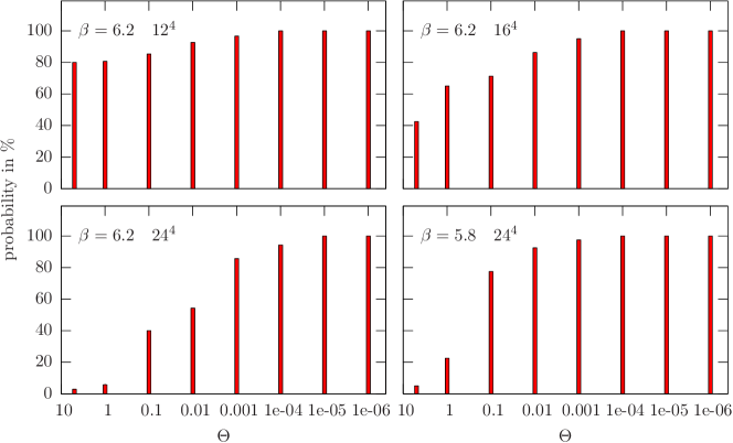
Figure A.4: In this figure we show the probability of having found (at intermediate values of $\Theta$) those copies which will result in the largest functional values after the gauge-fixing process has converged.

A.3 Speeding up the inversion of the FP operator

For the solution of the linear system $M\boldsymbol{\phi}=\boldsymbol{\psi}_{c}$ with symmetric matrix $M$, the conjugate gradient (CG) algorithm is the method of choice. Its convergence rate depends on the condition number, the ratio of largest to lowest eigenvalue of $M$. When all $U_{x,\mu}=\mathbb{1}$ obviously the FP operator is minus the Laplacian $\Delta$ with a diagonal color substructure. Thus instead of solving $M\boldsymbol{\phi}=\boldsymbol{\psi}_{c}$ one rather solves the transformed system

$$[M\Delta^{-1}]\,(\Delta\boldsymbol{\phi}\,)=\boldsymbol{\psi}_{c}$$

In this way the condition number is reduced, however, the price to pay is one extra matrix multiplication by $\Delta^{-1}$ per iteration cycle. In terms of CPU time this should be more than compensated by the reduction of iterations.

The pre-conditioned CG algorithm (PCG) can be described as follows:

initialize:

$$\boldsymbol{r}^{\,(0)} = \boldsymbol{\psi}-M\boldsymbol{\phi}^{\,(0)},\quad\boldsymbol{p}^{\,(0)}=\Delta^{-1}\,\boldsymbol{r}^{\,(0)},$$

$$\gamma^{(0)} = (\boldsymbol{p}^{\,(0)},\boldsymbol{r}^{\,(0)})$$

start do loop: $$k=0,1,\ldots$$

$$\boldsymbol{z}^{\,(k)} = M\boldsymbol{p}^{\,(k)},\quad\alpha^{(k)}=\gamma^{\,(k)}/(\boldsymbol{z}^{\,(k)},\boldsymbol{p}^{\,(k)})$$

$$\boldsymbol{\phi}^{\,(k+1)} = \boldsymbol{\phi}^{\,(k)}+\alpha^{(k)}\boldsymbol{p}^{\,(k)}$$

$$\boldsymbol{r}^{\,(k+1)} = \boldsymbol{r}^{\,(k)}-\alpha^{(k)}\boldsymbol{z}^{\,(k)}$$

$$\boldsymbol{z}^{\,(k+1)} = \Delta^{-1}\,\boldsymbol{r}^{\,(k+1)}$$

$$\gamma^{(k+1)} = (\boldsymbol{z}^{\,(k+1)},\boldsymbol{r}^{\,(k+1)})$$

if $$(\gamma^{(k+1)}<\varepsilon)\quad\textit{exit do loop}$$

$$\boldsymbol{p}^{\,(k+1)} = \boldsymbol{z}^{\,(k+1)}+\frac{\gamma^{(k+1)}}{\gamma^{(k)}}\boldsymbol{p}^{\,(k)}$$

end do loop

Here $(\cdot,\cdot)$ denotes the scalar product.

	CG		PCG		speed up
lattice	iter	CPU[sec]	iter	CPU[sec]	iter	CPU[sec]
$8^{4}$	1400	3.7	570	2.4	60%	35%
$16^{4}$	3900	240	1050	130	73%	46%
$32^{4}$	9900	13400	2250	3900	77%	71%

Table A.2: The average number of iterations and CPU time per processor (PE) using the CG and PCG algorithm to invert the FP operator are given for different lattice sizes. All inversions have been performed at $\beta=5.8$ with source $\delta^{bc}\exp(i\,k\!\cdot\!y)$ where $k=(1,0,0,0)$. To compare the different lattice sizes 4 PEs have always been used.

To perform the additional matrix multiplication with $\Delta^{-1}$ we used two fast Fourier transformations $\mathcal{F}$, due to $(-\Delta)^{-1}=\mathcal{F}^{-1}\,q^{-2}(k)\,\mathcal{F}$. The performance we achieved is presented in Table A.2. We conclude that on larger lattice sizes the reduction of iterations is about 70-75%, while the resulting reduction of CPU time depends on the lattice size. This is because we are using the fast Fourier transformations in a parallel CPU environment. If the ratio of used processors to the lattice size is small (see e.g. the data for $32^{4}$ lattice at this table), almost the same reductions of CPU time as for the number of iterations is achieved.

Further improvement may be achieved by using the multigrid Poisson solver to solve $\Delta\boldsymbol{z}^{\,(k)}=\boldsymbol{r}^{\,(k)}$. This method is supposed to perform better on parallel machines. Perhaps a further improvement is possible by using as pre-conditioning matrix $\widetilde{M}^{-1}=-\Delta^{-1}-\Delta^{-1}M_{1}\Delta^{-1}+\ldots$ which is an approximation of the FP operator $M=-\Delta+M_{1}$ to a given order Zwa [94] (see also FN04a ). However, the larger the order, the more matrix multiplications per iteration cycle are required. This may reduce the overall performance. We have not checked so far which is the optimal order.

References

- A+ [97] Aiso, H.; et al.: Towards understanding of confinement of gluons. In: Nucl. Phys. Proc. Suppl., volume 53:pp. 570–573, 1997.
- [2] Atkinson, D.; Bloch, J. C. R.: QCD in the infrared with exact angular integrations. In: Mod. Phys. Lett., volume A13:pp. 1055–1062, 1998. hep-ph/9802239.
- [3] Atkinson, D.; Bloch, J. C. R.: Running coupling in non-perturbative QCD. I: Bare vertices and y-max approximation. In: Phys. Rev., volume D58:p. 094036, 1998. hep-ph/9712459.
- ADFM [04] Alkofer, R.; Detmold, W.; Fischer, C. S.; Maris, P.: Analytic properties of the Landau gauge gluon and quark propagators. In: Phys. Rev., volume D70:p. 014014, 2004. hep-ph/0309077.
- ADJS [81] Atkinson, D.; Drohm, J. K.; Johnson, P. W.; Stam, K.: Nonperturbative confinement in Quantum Chromodynamics. 1. Study of an approximate equation of Mandelstam. In: J. Math. Phys., volume 22:p. 2704, 1981.
- AFLE [05] Alkofer, R.; Fischer, C. S.; Llanes-Estrada, F. J.: Vertex functions and infrared fixed point in Landau gauge SU(N) Yang-Mills theory. In: Phys. Lett., volume B611:pp. 279–288, 2005. hep-th/0412330.
- AFvS [03] Alkofer, R.; Fischer, C. S.; von Smekal, L.: Kugo-Ojima confinement criterion, Zwanziger-Gribov horizon condition, and infrared critical exponents in Landau gauge QCD, 2003. hep-ph/0301107.
- AHI+ [04] Aoki, S.; Hashimoto, S.; Ishizuka, N.; Kanaya, K.; Kuramashi, Y., editors: Lattice field theory. Proceedings, 21st International Symposium, Lattice 2003, Tsukuba, Japan, July 15-19, 2003. Nucl. Phys. B, Proc. Suppl. 129/130, 2004. Prepared for 21st International Symposium on Lattice Field Theory (LATTICE 2003), Tsukuba, Ibaraki, Japan, 15-19 July 2003, 950 pages.
- AJS [82] Atkinson, D.; Johnson, P. W.; Stam, K.: Nonperturbative confinement in Quantum Chromodynamics. 2. Mandelstam’s gluon propagator. In: J. Math. Phys., volume 23:p. 1917, 1982.
- AK+ [03] Ali Khan, A.; et al. (QCDSF): Accelerating the hybrid Monte Carlo algorithm. In: Phys. Lett., volume B564:pp. 235–240, 2003. hep-lat/0303026.
- AvS [01] Alkofer, R.; von Smekal, L.: The infrared behavior of QCD Green’s functions: Confinement, dynamical symmetry breaking, and hadrons as relativistic bound states. In: Phys. Rept., volume 353:p. 281, 2001. hep-ph/0007355.
- AvSW [01] Alkofer, R.; von Smekal, L.; Watson, P.: The Kugo-Ojima confinement criterion from Dyson-Schwinger equations. In: , 2001. hep-ph/0105142.
- [13] Boucaud, P.; et al.: Lattice calculation of corrections to and of in the scheme. In: JHEP, volume 04:p. 006, 2000. hep-ph/0003020.
- [14] Boucaud, Ph.; et al.: Consistent OPE description of gluon two point and three point Green function? In: Phys. Lett., volume B493:pp. 315–324, 2000. hep-ph/0008043.
- B+ [01] Boucaud, Ph.; et al.: Testing Landau gauge OPE on the lattice with a condensate. In: Phys. Rev., volume D63:p. 114003, 2001. hep-ph/0101302.
- B+ [03] Boucaud, Ph.; et al.: The strong coupling constant at small momentum as an instanton detector. In: JHEP, volume 04:p. 005, 2003. hep-ph/0212192.
- [17] Bodwin, G.; et al., editors: Lattice field theory. Proceedings, 22nd International Symposium, Lattice 2004, Batavia, USA, June 21-26, 2004. Nucl. Phys. B, Proc. Suppl. 140, 1-896, 2005. Prepared for 22nd International Symposium on Lattice Field Theory (Lattice 2004), Batavia, Illinois, 21-26 June 2004.
- [18] Boucaud, Ph.; et al.: The infrared behaviour of the pure Yang-Mills Green functions, 2005. hep-ph/0507104.
- [19] Boucaud, Ph.; et al.: Large momentum behavior of the ghost propagator in SU(3) lattice gauge theory. In: Phys. Rev., volume D72:p. 114503, 2005.
- [20] Bowman, P. O.; et al.: Unquenched quark propagator in Landau gauge. In: Phys. Rev., volume D71:p. 054507, 2005. hep-lat/0501019.
- [21] Boucaud, Ph.; et al.: Is the QCD ghost dressing function finite at zero momentum?, 2006. hep-ph/0604056.
- [22] Boucaud, Ph.; et al.: Non-perturbative power corrections to ghost and gluon propagators. In: JHEP, volume 01:p. 037, 2006. hep-lat/0507005.
- [23] Boucaud, Ph.; et al.: Short comment about the lattice gluon propagator at vanishing momentum, 2006. hep-lat/0602006.
- Bau [85] Baulieu, L.: Perturbative gauge theories. In: Phys. Rept., volume 129:p. 1, 1985.
- BBL+ [99] Bonnet, F. D. R.; Bowman, P. O.; Leinweber, D. B.; Williams, A. G.; Richards, D. G.: Discretisation errors in Landau gauge on the lattice. In: Austral. J. Phys., volume 52:pp. 939–948, 1999. hep-lat/9905006.
- BBL+ [01] Bonnet, F. D. R.; Bowman, P. O.; Leinweber, D. B.; Williams, A. G.; Zanotti, J. M.: Infinite volume and continuum limits of the Landau-gauge gluon propagator. In: Phys. Rev., volume D64:p. 034501, 2001. hep-lat/0101013.
- BBL+ [02] Bonnet, F. D. R.; Bowman, P. O.; Leinweber, D. B.; Williams, A. G.; Zhang, J. (CSSM Lattice): Overlap quark propagator in Landau gauge. In: Phys. Rev., volume D65:p. 114503, 2002. hep-lat/0202003.
- BBLW [00] Bonnet, F. D. R.; Bowman, P. O.; Leinweber, D. B.; Williams, A. G.: Infrared behavior of the gluon propagator on a large volume lattice. In: Phys. Rev., volume D62:p. 051501, 2000. hep-lat/0002020.
- BBMPM [05] Bogolubsky, I. L.; Burgio, G.; Müller-Preussker, M.; Mitrjushkin, V. K.: Landau gauge ghost and gluon propagators in SU(2) lattice gauge theory: Gribov ambiguity revisited, 2005. hep-lat/0511056.
- BCLM [03] Bloch, J. C. R.; Cucchieri, A.; Langfeld, K.; Mendes, T.: Running coupling constant and propagators in SU(2) Landau gauge. In: Nucl. Phys. Proc. Suppl., volume 119:pp. 736–738, 2003. hep-lat/0209040.
- BCLM [04] Bloch, J. C. R.; Cucchieri, A.; Langfeld, K.; Mendes, T.: Propagators and running coupling from SU(2) lattice gauge theory. In: Nucl. Phys., volume B687:pp. 76–100, 2004. hep-lat/0312036.
- BHL+ [04] Bowman, P. O.; Heller, U. M.; Leinweber, D. B.; Parappilly, M. B.; Williams, A. G.: Unquenched gluon propagator in landau gauge. In: Phys. Rev., volume D70:p. 034509, 2004. hep-lat/0402032.
- BHL+ [05] Bowman, P. O.; Heller, U. M.; Leinweber, D. B.; Williams, A. G.; Zhang, J. B.: Quark propagator from LQCD and its physical implications. In: Lect. Notes Phys., volume 663:pp. 17–63, 2005.
- BHW [02] Bowman, P. O.; Heller, U. M.; Williams, A. G.: Lattice quark propagator with staggered quarks in Landau and Laplacian gauges. In: Phys. Rev., volume D66:p. 014505, 2002. hep-lat/0203001.
- BIMMP [04] Bakeev, T. D.; Ilgenfritz, E.-M.; Mitrjushkin, V. K.; Müller-Preussker, M.: On practical problems to compute the ghost propagator in SU(2) lattice gauge theory. In: Phys. Rev., volume D69:p. 074507, 2004. hep-lat/0311041.
- [36] Boucaud, Ph.; Leroy, J. P.; Micheli, J.; Pene, O.; Roiesnel, C.: Lattice calculation of alpha(s) in momentum scheme. In: JHEP, volume 10:p. 017, 1998. hep-ph/9810322.
- [37] Boucaud, Ph.; Leroy, J. P.; Micheli, J.; Pene, O.; Roiesnel, C.: Three-loop beta function and non-perturbative alpha(s) in asymmetric momentum scheme. In: JHEP, volume 12:p. 004, 1998. hep-ph/9810437.
- Blo [01] Bloch, J. C. R.: Multiplicative renormalizability of gluon and ghost propagators in QCD. In: Phys. Rev., volume D64:p. 116011, 2001. hep-ph/0106031.
- Blo [02] Bloch, J. C. R.: Multiplicative renormalizability and quark propagator. In: Phys. Rev., volume D66:p. 034032, 2002. hep-ph/0202073.
- BP [89] Brown, N.; Pennington, M. R.: Studies of confinement: How the gluon propagates. In: Phys. Rev., volume D39:p. 2723, 1989.
- BPS [93] Bernard, C. W.; Parrinello, C.; Soni, A.: The gluon propagator in momentum space. In: Nucl. Phys. Proc. Suppl., volume 30:pp. 535–538, 1993. hep-lat/9211020.
- BPS [94] Bernard, Claude W.; Parrinello, C.; Soni, A.: A lattice study of the gluon propagator in momentum space. In: Phys. Rev., volume D49:pp. 1585–1593, 1994. hep-lat/9307001.
- BRS [75] Becchi, C.; Rouet, A.; Stora, R.: Renormalization of the abelian Higgs-Kibble model. In: Commun. Math. Phys., volume 42:pp. 127–162, 1975.
- BRS [76] Becchi, C.; Rouet, A.; Stora, R.: Renormalization of gauge theories. In: Annals Phys., volume 98:pp. 287–321, 1976.
- BW [87] Brown, F. R.; Woch, T. J.: Overrelaxed heat bath and Metropolis algorithms for accelerating pure gauge Monte Carlo calculations. In: Phys. Rev. Lett., volume 58:p. 2394, 1987.
- CG [79] Celmaster, W.; Gonsalves, R. J.: The renormalization prescription dependence of the QCD coupling constant. In: Phys. Rev., volume D20:p. 1420, 1979.
- Che [97] Chetyrkin, K. G.: Quark mass anomalous dimension to . In: Phys. Lett., volume B404:pp. 161–165, 1997. hep-ph/9703278.
- Che [05] Chetyrkin, K. G.: Four-loop renormalization of QCD: Full set of renormalization constants and anomalous dimensions. In: Nucl. Phys., volume B710:pp. 499–510, 2005. hep-ph/0405193.
- CM [82] Cabibbo, N.; Marinari, E.: A new method for updating SU(N) matrices in computer simulations of gauge theories. In: Phys. Lett., volume B119:pp. 387–390, 1982.
- CM [98] Cucchieri, A.; Mendes, T.: A multigrid implementation of the Fourier acceleration method for Landau gauge fixing. In: Phys. Rev., volume D57:pp. 3822–3826, 1998. hep-lat/9711047.
- CM [06] Cucchieri, A.; Mendes, T.: Infrared behavior of gluon and ghost propagators from asymmetric lattices, 2006. hep-lat/0602012.
- CMM [04] Cucchieri, A.; Mendes, T.; Mihara, A.: Numerical study of the ghost-gluon vertex in Landau gauge. In: JHEP, volume 12:p. 012, 2004. hep-lat/0408034.
- CMT [05] Cucchieri, A.; Mendes, T.; Taurines, A. R.: Positivity violation for the lattice Landau gluon propagator. In: Phys. Rev., volume D71:p. 051902, 2005. hep-lat/0406020.
- Col [84] Collins, J. C.: Renormalization. Cambridge University Press, 1984.
- CR [00] Chetyrkin, K. G.; Retey, A.: Renormalization and running of quark mass and field in the regularization invariant and MS-bar schemes at three and four loops. In: Nucl. Phys., volume B583:pp. 3–34, 2000. hep-ph/9910332.
- Cre [83] Creutz, M.: Quarks, Gluons and Lattices. Cambridge Monographs On Mathematical Physics. Cambridge, Uk: University Press, 1983. 169 pages.
- Cre [87] Creutz, M.: Overrelaxation and Monte Carlo simulation. In: Phys. Rev., volume D36:p. 515, 1987.
- Cuc [97] Cucchieri, A.: Gribov copies in the minimal Landau gauge: The influence on gluon and ghost propagators. In: Nucl. Phys., volume B508:pp. 353–370, 1997. hep-lat/9705005.
- Cuc [98] Cucchieri, A.: Numerical study of the fundamental modular region in the minimal Landau gauge. In: Nucl. Phys., volume B521:pp. 365–379, 1998. hep-lat/9711024.
- CZ [02] Cucchieri, A.; Zwanziger, D.: Numerical study of gluon propagator and confinement scenario in minimal Coulomb gauge. In: Phys. Rev., volume D65:p. 014001, 2002. hep-lat/0008026.
- D+ [88] Davies, C. T. H.; et al.: Fourier acceleration in lattice gauge theories. 1. Landau gauge fixing. In: Phys. Rev., volume D37:p. 1581, 1988.
- Dav [02] Davies, C.: Lattice QCD, pp. 105–146. Scottish Graduate Textbook Series, Institute of Physics 2002. St. Andrews 2001, Heavy flavour physics edition, 2002. Lectures given at 55th Scottish Universities Summer School in Physics: Heavy Flavor Physics, St. Andrews, Scotland, 7-23, hep-lat/0506036.
- Dav [05] Davies, C.: Lattice QCD - A guide for people who want results, 2005. hep-lat/0509046.
- DH [87] Damgaard, P. H.; Hüffel, H.: Stochastic quantization. In: Phys. Rept., volume 152:p. 227, 1987.
- DKPR [87] Duane, S.; Kennedy, A. D.; Pendleton, B. J.; Roweth, D.: Hybrid monte carlo. In: Phys. Lett., volume B195:pp. 216–222, 1987.
- E+ [04] Eidelman, S.; et al. (Particle Data Group): Review of Particle Physics. In: Phys. Lett., volume B592:p. 1, 2004. URL http://pdg.lbl.gov.
- ERV [94] Ebert, D.; Reinhardt, H.; Volkov, M. K.: Effective hadron theory of QCD. In: Prog. Part. Nucl. Phys., volume 33:pp. 1–120, 1994.
- ET [93] Efron, B.; Tibshirani, R. J.: An introduction to the Bootstrap. Chapman & Hall, 1993.
- FA [02] Fischer, C. S.; Alkofer, R.: Infrared exponents and running coupling of SU(N) Yang-Mills theories. In: Phys. Lett., volume B536:pp. 177–184, 2002. hep-ph/0202202.
- FA [03] Fischer, C. S.; Alkofer, R.: Non-perturbative propagators, running coupling and dynamical quark mass of Landau gauge QCD. In: Phys. Rev., volume D67:p. 094020, 2003. hep-ph/0301094.
- FAC+ [06] Fischer, C. S.; Alkofer, R.; Cassing, W.; Llanes-Estrada, F.; Watson, P.: Studying unquenching effects in QCD with Dyson-Schwinger equations. In: Nucl. Phys. Proc. Suppl., volume 153:pp. 90–97, 2006. hep-ph/0511147.
- FAR [02] Fischer, C. S.; Alkofer, R.; Reinhardt, H.: The elusiveness of infrared critical exponents in Landau gauge Yang-Mills theories. In: Phys. Rev., volume D65:p. 094008, 2002. hep-ph/0202195.
- Fey [48] Feynman, R. P.: Space-time approach to nonrelativistic quantum mechanics. In: Rev. Mod. Phys., volume 20:pp. 367–387, 1948.
- FGA [06] Fischer, C. S.; Grüter, B.; Alkofer, R.: Solving coupled Dyson-Schwinger equations on a compact manifold. In: Ann. Phys., volume 321:pp. 1918–1938, 2006. hep-ph/0506053.
- FH [84] Fabricius, K.; Haan, O.: Heat bath method for the twisted Eguchi-Kawai model. In: Phys. Lett., volume B143:p. 459, 1984.
- Fis [03] Fischer, C. S.: Non-perturbative propagators, running coupling and dynamical mass generation in ghost - antighost symmetric gauges in QCD. Ph.D. thesis, Tübingen University, 2003. hep-ph/0304233.
- FJ [98] Frigo, M.; Johnson, S. G.: FFTW: An adaptive software architecture for the FFT. In: Proc. 1998 IEEE Intl. Conf. Acoustics Speech and Signal Processing, volume 3, pp. 1381–1384. IEEE, 1998.
- FLS [72] Fujikawa, K.; Lee, B. W.; Sanda, A. I.: Generalized renormalizable gauge formulation of spontaneously broken gauge theories. In: Phys. Rev., volume D6:pp. 2923–2943, 1972.
- [79] Furui, S.; Nakajima, H.: Infrared features of the Landau gauge QCD. In: Phys. Rev., volume D69:p. 074505, 2004. hep-lat/0305010.
- [80] Furui, S.; Nakajima, H.: What the Gribov copy tells about confinement and the theory of dynamical chiral symmetry breaking. In: Phys. Rev., volume D70:p. 094504, 2004. hep-lat/0403021.
- [81] Furui, S.; Nakajima, H.: Infrared features of KS fermion and Wilson fermion in lattice Landau gauge QCD, 2005. hep-lat/0503029.
- [82] Furui, S.; Nakajima, H.: The running coupling in lattice Landau gauge with unquenched Wilson fermion and KS fermion. In: PoS, volume LAT2005:p. 291, 2005. hep-lat/0509035.
- [83] Furui, S.; Nakajima, H.: Effects of the quark field on the ghost propagator of lattice landau gauge QCD, 2006. hep-lat/0602027.
- [84] Furui, S.; Nakajima, H.: Unquenched Kogut-Susskind quark propagator in lattice Landau gauge QCD. In: Phys. Rev., volume D73:p. 074503, 2006. hep-lat/0511045.
- FP [67] Faddeev, L. D.; Popov, V. N.: Feynman diagrams for the Yang-Mills field. In: Phys. Lett., volume B25:pp. 29–30, 1967.
- FP [06] Fischer, C. S.; Pennington, M. R.: Finite volume effects in a quenched lattice-QCD quark propagator. In: Phys. Rev., volume D73:p. 034029, 2006. hep-ph/0512233.
- FWC [05] Fischer, C. S.; Watson, P.; Cassing, W.: Probing unquenching effects in the gluon polarisation in light mesons. In: Phys. Rev., volume D72:p. 094025, 2005. hep-ph/0509213.
- G+ [89] Gupta, R.; et al.: QCD with dynamical Wilson fermions. In: Phys. Rev., volume D40:p. 2072, 1989.
- G+ [04] Göckeler, M.; et al. (QCDSF): Determination of light and strange quark masses from full lattice QCD, 2004. hep-ph/0409312.
- G+ [06] Göckeler, M.; et al. (QCDSF–UKQCD): A determination of the Lambda parameter from full lattice QCD. In: Phys. Rev., volume D73:p. 014513, 2006. hep-ph/0502212.
- Geh [02] Gehrmann, B.: The step scaling function of QCD at negative flavor number. Ph.D. thesis, Humboldt University Berlin, 2002. hep-lat/0207016.
- GHP+ [05] Göckeler, M.; Horsley, R.; Pleiter, D.; Rakow, P. E. L.; Schierholz, G. (QCDSF): A lattice determination of moments of unpolarised nucleon structure functions using improved Wilson fermions. In: Phys. Rev., volume D71:p. 114511, 2005. hep-ph/0410187.
- GJ [87] Glimm, J.; Jaffe, A. M.: Quantum Physics. A Functional Integral Point of View. Springer-Verlag New York Inc., 2nd edition, 1987. 535 pages.
- GKW [05] Ghiotti, M.; Kalloniatis, A. C.; Williams, A. G.: Landau gauge Jacobian and BRST symmetry. In: Phys. Lett., volume B628:pp. 176–182, 2005. hep-th/0509053.
- GLR [04] Gattnar, J.; Langfeld, K.; Reinhardt, H.: Signals of confinement in Green functions of SU(2) Yang-Mills theory. In: Phys. Rev. Lett., volume 93:p. 061601, 2004. hep-lat/0403011.
- GLT+ [87] Gottlieb, S.; Liu, W.; Toussaint, D.; Renken, R. L.; Sugar, R. L.: Hybrid molecular dynamics algorithms for the numerical simulation of Quantum Chromodynamics. In: Phys. Rev., volume D35:pp. 2531–2542, 1987.
- GO [03] Greensite, J.; Olejnik, S.: Coulomb energy, vortices, and confinement. In: Phys. Rev., volume D67:p. 094503, 2003. hep-lat/0302018.
- Gre [03] Greensite, J.: The confinement problem in lattice gauge theory. In: Prog. Part. Nucl. Phys., volume 51:p. 1, 2003. hep-lat/0301023.
- Gri [78] Gribov, V. N.: Quantization of non-Abelian gauge theories. In: Nucl. Phys., volume B139:p. 1, 1978.
- Gup [97] Gupta, R.: Introduction to lattice QCD. In: Probing the standard model of particle interactions, Pt. 2 (Les Houches 1997), pp. 83–219, 1997. Lectures given at the LXVIII Les Houches Summer School, July 28–Sept 5 1997, hep-lat/9807028.
- [101] Gross, D. J.; Wilczek, F.: Asymptotically free gauge theories. 1. In: Phys. Rev., volume D8:pp. 3633–3652, 1973.
- [102] Gross, D. J.; Wilczek, F.: Ultraviolet behavior of non-abelian gauge theories. In: Phys. Rev. Lett., volume 30:pp. 1343–1346, 1973.
- Haa [92] Haag, R.: Local Quantum Physics: Fields, Particles, Algebras. Springer-Verlag Berlin, 1992. (Texts and monographs in physics), Corrected 2nd Printing 1993, 356p.
- Has [98] Hasenfratz, P.: The theoretical background and properties of perfect actions. In: , 1998. Prepared for Advanced Summer School on Nonperturbative Quantum Field Physics, Peniscola, Spain, 2-6 Jun 1997. In *Peniscola 1997, Non-perturbative quantum field physics* 137-199, hep-lat/9803027.
- Hua [92] Huang, K.: Quarks, leptons and gauge fields. Singapore, Singapore: World Scientific Publishing Co. Pte. Ltd., 1992. 333 pages.
- IMM [05] Irving, A.; McNeile, C.; Michael, C., editors: Lattice field theory. Proceedings, 23st International Symposium, Lattice 2005, Trinity College, Dublin, Ireland, 25-30 July 2005. PoS(LAT2005), 2005. Prepared for 23st International Symposium on Lattice Field Theory (LATTICE 2005), Trinity College, Dublin, Ireland, 25-30 July 2005.
- IMPSS [06] Ilgenfritz, E. M.; Müller-Preussker, M.; Sternbeck, A.; Schiller, A.: Gauge-variant propagators and the running coupling from lattice QCD. In: Sense of Beauty in Physics; Festschrift in honor of Adriano Di Giacomo’s 70-th birthday, 2006. January 26-27, 2006, Pisa, Italy, hep-lat/0601027.
- IT [76] Iofa, M. Z.; Tyutin, I. V.: Gauge invariance of spontaneously broken nonabelian theories in the Bogolyubov-Parasiuk-Hepp-Zimmerman method. (in russian). In: Teor. Mat. Fiz., volume 27:pp. 38–47, 1976.
- IZ [80] Itzykson, C.; Zuber, J.: Quantum field theory. McGraw-Hill Inc., 1980. 705 pages.
- JW [04] James, F.; Winkler, M.: MINUIT. CERN, May 2004. URL http://www.cern.ch/minuit.
- Kak [93] Kaku, M.: Quantum field theory: A modern introduction. New York, USA: Oxford University Press, 1993.
- Käl [52] Källen, G.: In: Helv. Phys. Acta, volume 25:p. 417, 1952.
- Kle [92] Klevansky, S. P.: The Nambu-Jona-Lasinio model of quantum chromodynamics. In: Rev. Mod. Phys., volume 64:pp. 649–708, 1992.
- Kne [99] Knechtli, F.: The static potential in the SU(2) Higgs model. Ph.D. thesis, Humboldt University Berlin, 1999. hep-lat/9910044.
- KNS [81] Kawai, H.; Nakayama, R.; Seo, K.: Comparison of the lattice Lambda parameter with the continuum Lambda parameter in massless QCD. In: Nucl. Phys., volume B189:p. 40, 1981.
- KO [79] Kugo, T.; Ojima, I.: Local covariant operator formalism of nonabelian gauge theories and quark confinement problem. In: Prog. Theor. Phys. Suppl., volume 66:p. 1, 1979.
- Kog [83] Kogut, J. B.: A review of the lattice gauge theory approach to quantum chromodynamics. In: Rev. Mod. Phys., volume 55:p. 775, 1983.
- KP [85] Kennedy, A. D.; Pendleton, B. J.: Improved heat bath method for Monte Carlo calculations in lattice gauge theories. In: Phys. Lett., volume B156:pp. 393–399, 1985.
- KU [82] Kugo, T.; Uehara, S.: General procedure of gauge fixing based on BRS invariance principle. In: Nucl. Phys., volume B197:p. 378, 1982.
- Kug [95] Kugo, T.: The universal renormalization factors Z(1) / Z(3) and color confinement condition in non-Abelian gauge theory, 1995. hep-th/9511033.
- KvSW [05] Kalloniatis, A. C.; von Smekal, L.; Williams, A. G.: Curci-Ferrari mass and the Neuberger problem. In: Phys. Lett., volume B609:pp. 424–429, 2005. hep-lat/0501016.
- Leh [54] Lehmann, H.: On the properties of propagation functions and renormalization contants of quantized fields. In: Nuovo Cim., volume 11:pp. 342–357, 1954.
- Lep [00] Lepage, G. P.: Lattice QCD for Novices. In: Proceedings of HUGS 98, edited by J.L. Goity, World Scientific, 2000. hep-lat/0506036.
- [124] Lehoucq, R.; Maschhoff, K.; Sorensen, D.; Yang, C.: ARPACK SOFTWARE. URL http://www.caam.rice.edu/software/ARPACK/.
- LRG [02] Langfeld, K.; Reinhardt, H.; Gattnar, J.: Gluon propagators and quark confinement. In: Nucl. Phys., volume B621:pp. 131–156, 2002. hep-ph/0107141.
- LSSW [96] Lüscher, M.; Sint, S.; Sommer, R.; Weisz, P.: Chiral symmetry and O(a) improvement in lattice QCD. In: Nucl. Phys., volume B478:pp. 365–400, 1996. hep-lat/9605038.
- LSWP [98] Leinweber, D. B.; Skullerud, J. I.; Williams, A. G.; Parrinello, C. (UKQCD): Gluon propagator in the infrared region. In: Phys. Rev., volume D58:p. 031501, 1998. hep-lat/9803015.
- LSWP [99] Leinweber, D. B.; Skullerud, J. I.; Williams, A. G.; Parrinello, C. (UKQCD): Asymptotic scaling and infrared behavior of the gluon propagator. In: Phys. Rev., volume D60:p. 094507, 1999. hep-lat/9811027.
- Lüs [03] Lüscher, M.: Lattice QCD: From quark confinement to asymptotic freedom. In: Annales Henri Poincare, volume 4:pp. S197–S210, 2003. Plenary talk given at International Conference on Theoretical Physics (TH 2002), Paris, France, 22-26 Jul 2002, hep-ph/0211220.
- LvS [02] Lerche, C.; von Smekal, L.: On the infrared exponent for gluon and ghost propagation in Landau gauge QCD. In: Phys. Rev., volume D65:p. 125006, 2002. hep-ph/0202194.
- LW [85] Luscher, M.; Weisz, P.: On-shell improved lattice gauge theories. In: Commun. Math. Phys., volume 97:p. 59, 1985.
- Man [79] Mandelstam, S.: Approximation scheme for QCD. In: Phys. Rev., volume D20:p. 3223, 1979.
- MM [94] Montvay, I.; Münster, G.: Quantum fields on a lattice. Cambridge University Press, 1994. 491 pages.
- MMS [95] Marenzoni, P.; Martinelli, G.; Stella, N.: The gluon propagator on a large volume, at . In: Nucl. Phys., volume B455:pp. 339–356, 1995. hep-lat/9410011.
- MMST [93] Marenzoni, P.; Martinelli, G.; Stella, N.; Testa, M.: High statistics study of the gluon propagator in the Landau gauge at . In: Phys. Lett., volume B318:pp. 511–516, 1993.
- MO [87] Mandula, J. E.; Ogilvie, M.: The gluon is massive: a lattice calculation of the gluon propagator in the Landau gauge. In: Phys. Lett., volume B185:pp. 127–132, 1987.
- [137] Mandula, J. E.; Ogilvie, M.: Efficient gauge fixing via overrelaxation. In: Phys. Lett., volume B248:pp. 156–158, 1990.
- [138] Mandula, J. E.; Ogilvie, M. C.: A possible resolution of the lattice Gribov ambiguity. In: Phys. Rev., volume D41:p. 2586, 1990.
- MP [78] Marciano, W. J.; Pagels, H.: Quantum chromodynamics: A review. In: Phys. Rept., volume 36:p. 137, 1978.
- MR [03] Maris, P.; Roberts, C. D.: Dyson-schwinger equations: A tool for hadron physics. In: Int. J. Mod. Phys., volume E12:pp. 297–365, 2003. nucl-th/0301049.
- Mut [98] Muta, T.: Foundations of quantum chromodynamics (2nd edition). In: World Sci. Lect. Notes Phys., volume 57:pp. 1–409, 1998.
- Nak [66] Nakishi, N.: Covariant quantization of the electromagnetic field in the Landau gauge. In: Prog. Theor. Phys., volume 35:p. 1111, 1966.
- Neu [87] Neuberger, H.: Nonperturbative BRS invariance and the Gribov problem. In: Phys. Lett., volume B183:p. 337, 1987.
- [144] Nakajima, H.; Furui, S.: Numerical tests of the Kugo-Ojima color confinement criterion, 2000. hep-lat/0006002.
- [145] Nakajima, H.; Furui, S.: Test of the Kugo-Ojima confinement criterion in the lattice Landau gauge. In: Nucl. Phys. Proc. Suppl., volume 83:pp. 521–523, 2000. hep-lat/9909008.
- [146] Nakajima, H.; Furui, S.: Infrared features of the lattice Landau gauge QCD. In: Nucl. Phys. Proc. Suppl., volume 129:pp. 730–732, 2004. hep-lat/0309165.
- [147] Nakajima, H.; Furui, S.: Numerical study of lattice Landau gauge QCD and the Gribov copy problem, 2004. hep-lat/0408001.
- NO [90] Nakanishi, N.; Ojima, I.: Covariant operator formalism of gauge theories and quantum gravity. In: World Sci. Lect. Notes Phys., volume 27:pp. 1–434, 1990.
- NS [02] Necco, S.; Sommer, R.: The N(f) = 0 heavy quark potential from short to intermediate distances. In: Nucl. Phys., volume B622:pp. 328–346, 2002. hep-lat/0108008.
- Oeh [95] Oehme, R.: Analytic structure of amplitudes in gauge theories with confinement. In: Int. J. Mod. Phys., volume A10:pp. 1995–2014, 1995. hep-th/9412040.
- Oji [78] Ojima, I.: Observables and quark confinement in the covariant canonical formalism of the Yang-Mills theory. In: Nucl. Phys., volume B143:p. 340, 1978.
- Opp [30] Oppenheimer, J. R.: Note on the theory of the interaction of field and matter. In: Phys. Rev., volume 35:pp. 461–477, 1930.
- OS [73] Osterwalder, K.; Schrader, R.: Axioms for Euclidean Green’s functions. In: Commun. Math. Phys., volume 31:pp. 83–112, 1973.
- OS [75] Osterwalder, K.; Schrader, R.: Axioms for Euclidean Green’s functions. 2. In: Commun. Math. Phys., volume 42:p. 281, 1975.
- [155] Oliveira, O.; Silva, P. J.: Finite volume effects in the gluon propagator. In: PoS, volume LAT2005:p. 287, 2005. hep-lat/0509037.
- [156] Oliveira, O.; Silva, P. J.: The infrared Landau gauge gluon propagator from lattice QCD. In: AIP Conf. Proc., volume 756:pp. 290–292, 2005. hep-lat/0410048.
- P+ [06] Parappilly, Maria B.; et al.: Scaling behavior of quark propagator in full QCD. In: Phys. Rev., volume D73:p. 054504, 2006. hep-lat/0511007.
- Pol [73] Politzer, H. D.: Reliable perturbative results for strong interactions? In: Phys. Rev. Lett., volume 30:pp. 1346–1349, 1973.
- PS [95] Peskin, M. E.; Schroeder, D. V.: An Introduction to quantum field theory. Reading, USA: Addison-Wesley, 1995. 842 pages.
- PTVF [92] Press, W. H.; Teukolsky, S. A.; Vetterling, W. T.; Flannery, B. P.: Numerical Recipes in Fortran 77: The Art of Scientific Computing. Cambridge University Press, Cambridge (UK) and New York, 2nd edition, 1992. ISBN 0-521-43064-X.
- PW [81] Parisi, G.; Wu, Yong-shi: Perturbation theory without gauge fixing. In: Sci. Sin., volume 24:p. 483, 1981.
- Rei [89] Reisz, T.: Lattice gauge theory: renormalization to all orders in the loop expansion. In: Nucl. Phys., volume B318:p. 417, 1989.
- Rot [97] Rothe, H. J.: Lattice gauge theories: An introduction. In: World Sci. Lect. Notes Phys., volume 59:pp. 1–512, 1997.
- RS [00] Roberts, C. D.; Schmidt, S. M.: Dyson-Schwinger equations: Density, temperature and continuum strong QCD. In: Prog. Part. Nucl. Phys., volume 45:pp. S1–S103, 2000. nucl-th/0005064.
- RW [94] Roberts, C. D.; Williams, A. G.: Dyson-Schwinger equations and their application to hadronic physics. In: Prog. Part. Nucl. Phys., volume 33:pp. 477–575, 1994. hep-ph/9403224.
- SBK+ [03] Skullerud, J. I.; Bowman, P. O.; Kizilersu, A.; Leinweber, D. B.; Williams, A. G.: Nonperturbative structure of the quark gluon vertex. In: JHEP, volume 04:p. 047, 2003. hep-ph/0303176.
- Sch [04] Schleifenbaum, W.: The ghost-gluon vertex in Landau gauge Yang-Mills theory in four and three dimensions. Diploma thesis, TU-Darmstadt, December 2004.
- SIMP [06] Sternbeck, A.; Ilgenfritz, E.-M.; Müller-Preussker, M.: Spectral properties of the Landau gauge Faddeev-Popov operator in lattice gluodynamics. In: Phys. Rev., volume D73:p. 014502, 2006. hep-lat/0510109.
- [169] Sternbeck, A.; Ilgenfritz, E.-M.; Müller-Preussker, M.; Schiller, A.: The gluon and ghost propagator and the influence of Gribov copies. In: Nucl. Phys. Proc. Suppl., volume 140:pp. 653–655, 2005. hep-lat/0409125.
- [170] Sternbeck, A.; Ilgenfritz, E.-M.; Müller-Preussker, M.; Schiller, A.: The influence of Gribov copies on the gluon and ghost propagator. In: AIP Conf. Proc., volume 756:pp. 284–286, 2005. hep-lat/0412011.
- [171] Sternbeck, A.; Ilgenfritz, E.-M.; Müller-Preussker, M.; Schiller, A.: Studying the infrared region in Landau gauge QCD. In: PoS, volume LAT2005:p. 333, 2005. hep-lat/0509090.
- [172] Sternbeck, A.; Ilgenfritz, E.-M.; Müller-Preussker, M.; Schiller, A.: Towards the infrared limit in SU(3) Landau gauge lattice gluodynamics. In: Phys. Rev., volume D72:p. 014507, 2005. hep-lat/0506007.
- SIMPS [06] Sternbeck, A.; Ilgenfritz, E.-M.; Müller-Preussker, M.; Schiller, A.: Landau gauge ghost and gluon propagators and the Faddeev- Popov operator spectrum. In: Nucl. Phys. Proc. Suppl., volume 153:pp. 185–190, 2006. hep-lat/0511053.
- Sin [78] Singer, I. M.: Some remarks on the Gribov ambiguity. In: Commun. Math. Phys., volume 60:pp. 7–12, 1978.
- SK [02] Skullerud, J.; Kizilersu, A.: Quark-gluon vertex from lattice QCD. In: JHEP, volume 09:p. 013, 2002. hep-ph/0205318.
- Sla [72] Slavnov, A. A.: Ward identities in gauge theories. In: Theor. Math. Phys., volume 10:pp. 99–107, 1972.
- SLW [01] Skullerud, J.; Leinweber, D. B.; Williams, A. G.: Nonperturbative improvement and tree-level correction of the quark propagator. In: Phys. Rev., volume D64:p. 074508, 2001. hep-lat/0102013.
- Smi [02] Smit, J.: Introduction to quantum fields on a lattice: A robust mate, volume 15 of Cambridge lecture notes in physics. Cambridge University Press, Cambridge, 2002. ISBN: 0521890519.
- SMWA [04] Schleifenbaum, W.; Maas, A.; Wambach, J.; Alkofer, R.: The ghost-gluon vertex in Landau gauge Yang-Mills theory, 2004. hep-ph/0411060.
- SMWA [05] Schleifenbaum, W.; Maas, A.; Wambach, J.; Alkofer, R.: Infrared behaviour of the ghost-gluon vertex in Landau gauge Yang-Mills theory. In: Phys. Rev., volume D72:p. 014017, 2005. hep-ph/0411052.
- SO [04] Silva, P. J.; Oliveira, O.: Gribov copies, lattice QCD and the gluon propagator. In: Nucl. Phys., volume B690:pp. 177–198, 2004. hep-lat/0403026.
- [182] Silva, P. J.; Oliveira, O.: The IR gluon propagator from lattice QCD. In: PoS, volume LAT2005:p. 286, 2005. hep-lat/0509034.
- [183] Silva, P. J.; Oliveira, O.: On the infrared gluon propagator, 2005. hep-lat/0511043.
- Som [94] Sommer, R.: A new way to set the energy scale in lattice gauge theories and its applications to the static force and in SU(2) Yang-Mills theory. In: Nucl. Phys., volume B411:pp. 839–854, 1994. hep-lat/9310022.
- SS [96] Suman, H.; Schilling, K.: First lattice study of ghost propagators in SU(2) and SU(3) gauge theories. In: Phys. Lett., volume B373:pp. 314–318, 1996. hep-lat/9512003.
- SW [85] Sheikholeslami, B.; Wohlert, R.: Improved continuum limit lattice action for QCD with Wilson fermions. In: Nucl. Phys., volume B259:p. 572, 1985.
- SW [01] Skullerud, J. I.; Williams, A. G.: Quark propagator in Landau gauge. In: Phys. Rev., volume D63:p. 054508, 2001. hep-lat/0007028.
- SW [05] Stüben, H.; Wollny, S.: Using the mass storage system at ZIB within I3HP, 2005. hep-lat/0512008.
- Tay [71] Taylor, J. C.: Ward identities and charge renormalization of the Yang- Mills field. In: Nucl. Phys., volume B33:pp. 436–444, 1971.
- Tes [98] Testa, M.: Lattice gauge fixing, Gribov copies and BRST symmetry. In: Phys. Lett., volume B429:pp. 349–353, 1998. hep-lat/9803025.
- [191] ’t Hooft, G.: Renormalizable Lagrangians for massive Yang-Mills fields. In: Nucl. Phys., volume B35:pp. 167–188, 1971.
- [192] ’t Hooft, G.: Renormalization of massless Yang-Mills fields. In: Nucl. Phys., volume B33:pp. 173–199, 1971.
- tHV [72] ’t Hooft, G.; Veltman, M. J. G.: Regularization and renormalization of gauge fields. In: Nucl. Phys., volume B44:pp. 189–213, 1972.
- Tyu [75] Tyutin, I. V.: 1975. Lebedev Institute preprint N39.
- vB [92] van Baal, P.: More (thoughts on) Gribov copies. In: Nucl. Phys., volume B369:pp. 259–275, 1992.
- vSAH [97] von Smekal, L.; Alkofer, R.; Hauck, A.: The infrared behavior of gluon and ghost propagators in Landau gauge QCD. In: Phys. Rev. Lett., volume 79:pp. 3591–3594, 1997. hep-ph/9705242.
- vSHA [98] von Smekal, L.; Hauck, A.; Alkofer, R.: A solution to coupled Dyson-Schwinger equations for gluons and ghosts in Landau gauge. In: Ann. Phys., volume 267:p. 1, 1998. hep-ph/9707327.
- VW [91] Vogl, U.; Weise, W.: The Nambu and Jona Lasinio model: Its implications for hadrons and nuclei. In: Prog. Part. Nucl. Phys., volume 27:pp. 195–272, 1991.
- WA [01] Watson, P.; Alkofer, R.: Verifying the Kugo-Ojima confinement criterion in Landau gauge QCD. In: Phys. Rev. Lett., volume 86:p. 5239, 2001. hep-ph/0102332.
- Wei [83] Weisz, P.: Continuum limit improved lattice action for pure Yang-Mills theory. 1. In: Nucl. Phys., volume B212:p. 1, 1983.
- Wei [95] Weinberg, S.: The Quantum theory of fields. Vol. 1: Foundations. Cambridge, UK: University Press, 1995. 609 pages.
- Wei [96] Weinberg, S.: The Quantum theory of fields. Vol. 2: Modern Applications. Cambridge University Press, 1996. 489 pages.
- Wil [74] Wilson, K. G.: Confinement of quarks. In: Phys. Rev., volume D10:pp. 2445–2459, 1974.
- Wil [02] Williams, A. G.: QCD, gauge fixing, and the Gribov problem. In: Nucl. Phys. Proc. Suppl., volume 109A:pp. 141–145, 2002. hep-lat/0202010.
- Wil [03] Williams, A. G.: Nonperturbative QCD, gauge-fixing, Gribov copies, and the lattice. In: Prog. Theor. Phys. Suppl., volume 151:pp. 154–160, 2003. hep-lat/0304003.
- Wu [86] Wu, C. F. J.: Jackknife, bootstrap and other resampling plans in regression analysis. In: Annals of Statistics, volume 14:pp. 1261–1295, 1986.
- WW [84] Weisz, P.; Wohlert, R.: Continuum limit improved lattice action for pure Yang-Mills theory. 2. In: Nucl. Phys., volume B236:p. 397, 1984. Erratum-ibid.B247:544,1984.
- Z+ [05] Zhang, J. B.; et al.: Quark propagator in Landau and Laplacian gauges with overlap fermions. In: Phys. Rev., volume D71:p. 014501, 2005. hep-lat/0410045.
- ZBL+ [04] Zhang, J. B.; Bowman, Patrick O.; Leinweber, D. B.; Williams, A. G.; Bonnet, F. D. R. (CSSM Lattice): Scaling behavior of the overlap quark propagator in landau gauge. In: Phys. Rev., volume D70:p. 034505, 2004. hep-lat/0301018.
- Zwa [82] Zwanziger, D.: Nonperturbative modification of the Faddeev-Popov formula and banishment of the naive vacuum. In: Nucl. Phys., volume B209:p. 336, 1982.
- [211] Zwanziger, D.: Vanishing color magnetization in lattice Landau and Coulomb gauges. In: Phys. Lett., volume B257:pp. 168–172, 1991.
- [212] Zwanziger, D.: Vanishing of zero momentum lattice gluon propagator and color confinement. In: Nucl. Phys., volume B364:pp. 127–161, 1991.
- Zwa [92] Zwanziger, D.: Critical limit of lattice gauge theory. In: Nucl. Phys., volume B378:pp. 525–590, 1992.
- Zwa [93] Zwanziger, D.: Renormalizability of the critical limit of lattice gauge theory by BRS invariance. In: Nucl. Phys., volume B399:pp. 477–513, 1993.
- Zwa [94] Zwanziger, D.: Fundamental modular region, Boltzmann factor and area law in lattice gauge theory. In: Nucl. Phys., volume B412:pp. 657–730, 1994.
- Zwa [98] Zwanziger, D.: Renormalization in the coulomb gauge and order parameter for confinement in qcd. In: Nucl. Phys., volume B518:pp. 237–272, 1998.
- Zwa [02] Zwanziger, D.: Non-perturbative Landau gauge and infrared critical exponents in QCD. In: Phys. Rev., volume D65:p. 094039, 2002. hep-th/0109224.
- [218] Zwanziger, D.: No confinement without Coulomb confinement. In: Phys. Rev. Lett., volume 90:p. 102001, 2003. hep-lat/0209105.
- [219] Zwanziger, D.: Time-independent stochastic quantization, DS equations, and infrared critical exponents in QCD. In: Phys. Rev., volume D67:p. 105001, 2003. hep-th/0206053.
- Zwa [04] Zwanziger, D.: Non-perturbative Faddeev-Popov formula and infrared limit of QCD. In: Phys. Rev., volume D69:p. 016002, 2004. hep-ph/0303028.
Acknowledgments
First and foremost, I would like to thank my Ph.D. advisor Michael Müller-Preußker for the opportunity to work on this subject and the good support over the last years. The support from him stems from the time I began studying for my degree at the Humboldt-University Berlin. Also, I would like to thank him for the possibility to extend my stay within the PHA group half a year longer than planned before and for reading the manuscript.
Furthermore, I owe deep gratitude to Ernst–Michael Ilgenfritz for many helpful discussions and for careful reading several drafts of this thesis. His questioning mind contributed greatly to this project.
I also thank Giuseppe Burgio, Hilmar Forkel and Jan Volkholz for enlightening discussions and for proof reading parts of the manuscript. They delivered many useful comments and improving remarks. Furthermore, I would like to thank my former and present office mates Dirk Peschka and Peter Schemel for discussions and inspiring coffee breaks. It was also always a pleasure for me to have discussions with Dietmar Ebert all the years at Humboldt-University.
Also I am indebted to Hinnerk Stüben for contributing parts of the program code. Due to his expert knowledge I have learned a lot about efficient programming for high performance computing. This has enabled me to develop the simulation program for this study.
I also acknowledge valuable discussions and correspondence with Reinhard Alkofer, Christian Fischer, Valentin K. Mitrjushkin, Arwed Schiller and Lorenz von Smekal.
I wish to send a special thank to Anett for all her love she gave me during the years and her support while writing this thesis. I thank Nikola and wish the best for her degree.
I would also like to thank the Magisters for providing me Internet access at home all the time, in particular on weekends. This helped me to keep the simulations running all the time.
This work was supported by the DFG-funded graduate school GK 271 and by the SFB/Tr9. All simulations have been done on the IBM pSeries 690 at HLRN. I used configurations generated by the QCDSF collaboration which I could access in the framework of the I3 Hadron-Physics initiative (EU contract RII3-CT-2004-506078). I thank Gerrit Schierholz, Dirk Pleiter and Stefan Wollny for their help.