HIP-2006-41/TH

Plaquette expectation value and lattice free energy
of three-dimensional SU$(N_{\rm c})$ gauge theory

A. Hietanen^a,b, A. Kurkela^a,

^aTheoretical Physics Division, Department of Physical Sciences,
P.O.Box 64, FI-00014 University of Helsinki, Finland

^bHelsinki Institute of Physics,
P.O.Box 64, FI-00014 University of Helsinki, Finland

1 Introduction

The determination of QCD pressure up to order $g^{6}$ is a long-standing problem in finite-temperature field theory [1, 2, 3]. This is the first order where a coefficient of the weak-coupling expansion, due to infrared divergences, gets contributions from an infinite number of loop-diagrams and thus is non-perturbative.

However, at high enough temperatures ($T\gtrsim 2T_{c}$) the properties of finite-temperature QCD can be described by dimensionally reduced effective field theory methods [4, 5]. By integrating out temporal degrees of freedom a three-dimensional pure gauge theory, called magnetostatic QCD (MQCD), is constructed. This allows us to isolate all the divergences to MQCD and study it using lattice calculations. The integration out is most conveniently performed perturbatively in $\overline{\rm{MS}}$ scheme [6].

We can relate any lattice regularized quantities within MQCD to the continuum scheme ($\overline{\rm{MS}}$), because MQCD is super-renormalizable. There are ultraviolet divergences up to 4-loop level only [7]. Terms required in the conversion have been determined up to 3-loop level [8, 9]. Infrared divergences cause an additional complication in the 4-loop level. The computation requires an introduction of an IR cutoff, which then cancels once lattice and $\overline{\rm{MS}}$ results are subtracted. This computation has been carried out recently for $N_{\rm c}=3$ in [10] using stochastic perturbation theory.

In [11] the plaquette expectation value, which determines the non-perturbative contribution, was measured for $N_{\rm c}=3$. The purpose of this paper is to extend the results to study the $N_{\rm c}$-dependence of this observable. We carry out lattice measurements of the plaquette with $N_{\rm c}=2,3,4,5$ and $8$ to obtain the $N_{\rm c}$-dependence. We also get an independent approximation for the $N_{\rm c}=3$ result. This acts as a consistency check for the whole pressure calculation. Namely, we expect to see smooth $N_{\rm c}$-dependence in the observable.

Additionally, there are various other physical motivations to study the $N_{\rm c}$-dependence and especially the large-$N_{\rm c}$ limit of SU($N_{\rm c}$) gauge theories [12]. The limit $N_{\rm c}\rightarrow\infty$ simplifies the theory significantly, but nevertheless the phenomenology is in many ways similar to SU(3). These reasons have motivated numerous large-$N_{\rm c}$ limit studies on the lattice [13, 14].

The paper is organized as follows. In Sec. 2, we give the theoretical background of our study and specify the observable we consider. In Sec. 3 we present the numerical results of lattice Monte Carlo simulations. Conclusions are given in Sec. 4.

2 Theoretical setup

The ultimate interest of our study is Euclidean pure SU($N_{\rm c}$) Yang-Mills theory, defined in continuum dimensional regularization by

$$S_{\rm{E}}=\int\!\textrm{d}^{d}x\,\mathcal{L}_{\rm{E}},\quad\quad\mathcal{L}_{\rm{E}}=\frac{1}{2g_{3}^{2}}\sum_{k,l}\textrm{Tr}[F^{2}_{kl}],$$ (2.1)

where $d=3-2\epsilon$, $g_{3}^{2}$ is the gauge coupling, $k,l=1,\dots,d$, $F_{kl}=i[D_{k},D_{l}]$, $D_{k}=\partial_{k}-iA_{k}$, $A_{k}=A_{k}^{a}T^{a}$, and $T^{a}$ are Hermitean generators of SU($N_{\rm c}$) normalized such that $\textrm{Tr}[T^{a}T^{b}]=\delta^{ab}/2$. The vacuum energy density in $\overline{\rm{MS}}$ (suppressing Faddev-Popov and gauge fixing terms) is defined by

$$f_{\overline{\rm{MS}}}\equiv-\lim_{V\rightarrow\infty}\frac{1}{V}\ln\left[\int\!\mathcal{D}A_{k}\,\exp\left(-S_{\rm{E}}\right)\right]_{\overline{\rm{MS}}},$$ (2.2)

where $V$ denotes the $d$-dimensional volume. The use of the $\overline{\rm{MS}}$ dimensional regularization scheme removes any $1/\epsilon$ poles from the expression. In fact, using dimensional regularization the perturbative result vanishes, because there are no mass scales in the propagators and therefore the UV and IR divergences cancel each other. However, for dimensional reasons, the non-perturbative form of the free energy is

$$f_{\overline{\rm{MS}}}=g_{3}^{6}\left[A_{G}^{\prime}\ln\frac{\bar{\mu}}{g_{3}^{2}}+B_{G}^{\prime}\right],$$ (2.3)

where $\bar{\mu}$ is the $\overline{\rm{MS}}$ renormalization scheme scale parameter. The coefficient of the logarithm has been calculated by introducing a mass scale $m_{\rm{G}}^{2}$ for gluon and ghost propagators and sending $m_{\rm{G}}^{2}\rightarrow 0$ after the computation [3, 15]:

$$f_{\overline{\rm{MS}}}=-g_{3}^{6}\frac{d_{A}N_{\rm c}^{3}}{(4\pi)^{4}}\left[\left(\frac{43}{12}-\frac{157}{768}\pi^{2}\right)\ln\frac{\bar{\mu}}{2N_{\rm c}g_{3}^{2}}+B_{\rm{G}}(N_{\rm c})+\mathcal{O}(\epsilon)\right],$$ (2.4)

where $d_{A}=N_{\rm c}^{2}-1$. The non-perturbative constant part $B_{\rm{G}}$, which is a function of the number of colors, is what one would ultimately like to determine.

Using standard Wilson discretization, we can write the corresponding action on the lattice as

$$S_{a}=\beta\sum_{{\bf x}}\sum_{k<l}^{3}\left(1-\frac{1}{N_{\rm c}}\textrm{Re}\textrm{Tr}[P_{kl}({\bf x})]\right),$$ (2.5)

where $P_{kl}$ is the plaquette, $a$ is the lattice spacing and $\beta\equiv 2N_{\rm c}/(ag_{3}^{2})$. Hence the continuum limit is taken by $\beta\rightarrow\infty$. Analogously to $\overline{\rm{MS}}$, the free energy density is defined on the lattice as

$$f_{a}\equiv-\lim_{V\rightarrow\infty}\frac{1}{V}\ln\left[\int\!\mathcal{D}U_{k}\,\exp\left(-S_{a}\right)\right].$$ (2.6)

Dimensionally, the vacuum energy density consists of terms of the form $g_{3}^{2n}a^{n-3}$. Thus, approaching the continuum limit, we can relate $f_{a}$ and $f_{\overline{\rm{MS}}}$ as follows:

$$\Delta f \equiv f_{a}-f_{\overline{\rm{MS}}}$$ (2.7)

$$= C_{1}\frac{1}{a^{3}}\left(\ln\frac{1}{ag_{3}^{2}}+C_{1}^{\prime}\right)+C_{2}\frac{g_{3}^{2}}{a^{2}}+C_{3}\frac{g_{3}^{4}}{a}+C_{4}g_{3}^{6}\left(\ln\frac{1}{a\bar{\mu}}+C_{4}^{\prime}\right)+\mathcal{O}(g_{3}^{8}a).$$ (2.8)

Taking derivatives of Eq. (2.7) with respect to $g_{3}^{2}$ and using 3d rotational and translational symmetries on the lattice, we obtain the relation [11]

$$8\frac{d_{A}N_{\rm c}^{6}}{(4\pi)^{4}}B_{\rm{G}}(N_{\rm c})=\lim_{\beta\rightarrow\infty}\beta^{4}\left\{\langle 1-\frac{1}{N_{\rm c}}\textrm{Tr}[P]\rangle_{a}-\left[\frac{c_{1}}{\beta}+\frac{c_{2}}{\beta^{2}}+\frac{c_{3}}{\beta^{3}}+\frac{c_{4}}{\beta^{4}}(\ln\beta+c_{4}^{\prime})\right]\right\}.$$ (2.9)

The relations between $c_{i}$ and $C_{i}$ are

$$c_{1} =C_{1}/3 c_{2} =-\frac{2N_{\rm c}}{3}C_{2} c_{3} =-\frac{8N_{\rm c}^{2}}{3}C_{3}$$

$$c_{4} =-8N_{\rm c}^{3}C_{4} c_{4}^{\prime} =C_{4}^{\prime}-\frac{1}{3}-2\ln(2N_{\rm c}).$$ (2.10)

The first follows from a straightforward 1-loop computation:

$$c_{1}=\frac{d_{A}}{3}.$$ (2.11)

The 2-loop constant has been computed in three dimensions in [16] and can be written as

$$c_{2} = -\frac{2}{3}\frac{d_{A}N_{\rm c}^{2}}{(4\pi)^{2}}\left(\frac{4\pi^{2}}{3N_{\rm c}^{2}}+\frac{\Sigma^{2}}{4}-\pi\Sigma-\frac{\pi^{2}}{2}+4\kappa_{1}+\frac{2}{3}\kappa_{5}\right)$$ (2.12)

$$= d_{A}N_{\rm c}^{2}\left(0.03327444(8)-\frac{1}{18}\frac{1}{N_{\rm c}^{2}}\right),$$ (2.13)

where the coefficients $\Sigma$, $\kappa_{1}$ and $\kappa_{5}$ can be found in [7, 17]. The 3-loop term has been computed in three dimensions recently in Ref. [9]:

$$c_{3}=d_{A}N_{\rm c}^{4}\left(0.0147397(3)-0.04289464(7)\frac{1}{N_{\rm c}^{2}}+0.04978944(1)\frac{1}{N_{\rm c}^{4}}\right).$$ (2.14)

Because there is no $\bar{\mu}$ dependence in $f_{a}$, the value of $c_{4}$ is determined by $f_{\overline{\rm{MS}}}$,

$$c_{4}=0.000502301323d_{A}N_{\rm c}^{6}.$$ (2.15)

The four-loop free energy itself is an IR divergent quantity at in both $\overline{\rm{MS}}$ and lattice schemes. But the finite difference between them, $c_{4}^{\prime}$, can be defined by introducing the same IR cutoff, e.g. a gluon mass, to both schemes. The cutoff dependence then cancels out when the two schemes are compared. At present $c_{4}^{\prime}$ is known only for $N_{\rm c}=3$, for which it has been calculated using stochastic perturbation theory [10].

For later use we define the quantity

$$P_{G}(\beta,N_{\rm c})\equiv\frac{32\pi^{4}\beta^{4}}{d_{A}N_{\rm c}^{6}}\left\{\langle 1-\frac{1}{N_{\rm c}}\textrm{Tr}[P]\rangle_{a}-\left[\frac{c_{1}}{\beta}+\frac{c_{2}}{\beta^{2}}+\frac{c_{3}}{\beta^{3}}+\frac{c_{4}}{\beta^{4}}\ln\beta\right]\right\},$$ (2.16)

which is a normalized plaquette expectation value minus all the ultraviolet divergences. Hence,

$$B_{\rm{G}}(N_{\rm c})-\left(\frac{43}{12}-\frac{157}{768}\pi^{2}\right)c_{4}^{\prime}=P_{G}(\infty,N_{\rm c}).$$ (2.17)

Our goal here is to determine $P_{G}(\infty,N_{c})$. After the $N_{\rm c}$-dependence of $c_{4}^{\prime}$ has been determined by, e.g., stochastic perturbation theory, one has reached the final goal, the determination of $B_{G}(N_{c})$.

3 Lattice computations

The simulations were performed using Kennedy-Pendleton quasi heat bath (HB) [18] and overrelaxation (OR) algorithms. For the overrelaxation we used an algorithm which updates the whole matrix using singular value decomposition and performs very well for large $N_{\rm c}$ [19]. Lattices of size $N^{3}$, $N=24,\ldots,400$ were used.

For each HB update we performed one OR. The number of updated subgroups in HB for $N_{\rm c}=$ 3, 4, 5 and 8 were 3, 4, 8 and 24, respectively. These subgroups were chosen randomly for each update. After each of these cycles we measured the value of the plaquette. The integrated autocorrelation times were around 0.75. For SU(2) we used dedicated OR and HB algorithms, with a ratio of one OR step for each HB update. The autocorrelation time was around 0.6. The data sets used for SU(3) are the same as in [11].

The contribution of $B_{G}$ to the plaquette expectation value in Eq. (2.9) is about five orders of magnitude smaller than the leading order contribution. Thus we experience massive significance loss in the subtraction and the accuracy requirement makes the numerical computation demanding (Fig. 1).

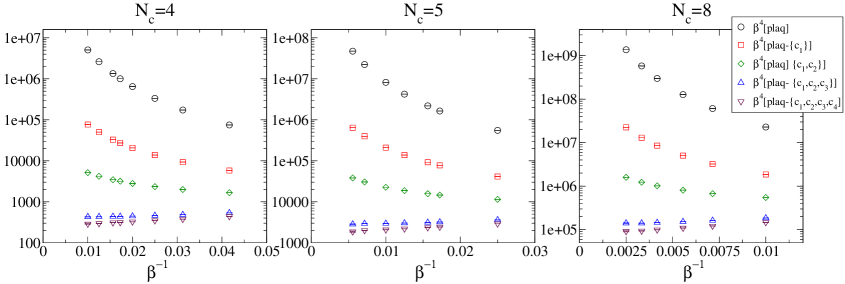
Figure 1: The significance loss due to the subtraction of ultraviolet divergences in the plaquette expectation value with different $N_{\rm c}$. Here “plaq”$\equiv\langle 1-\frac{1}{N_{\rm c}}\textrm{Tr}[P]\rangle$ and the symbols $c_{i}$ in curly brackets represent which subtractions of Eq. (2.9) have been taken into account.

The only physical scale in this problem is the correlation length of the lightest glueball, which according to [20] is $\sim 1/N_{\rm c}g_{3}^{2}$. The requirement, that this scale be in the reach of the lattice gives us the condition

$$a\ll\frac{1}{g_{3}^{2}N_{\rm c}}\ll Na,$$ (3.1)

which translates into

$$2N_{\rm c}^{2}\ll\beta\ll 2N_{\rm c}^{2}N.$$ (3.2)

Systematic errors due to the finite-volume effects turn out to be well under control. Because the theory is confining, we expect finite-volume effects to be exponentially suppressed when the condition (3.2) is fulfilled. As seen in Fig. 2, the finite-volume effects are no longer visible within our resolution when $\beta\lesssim 0.2N_{\rm c}^{2}N$.

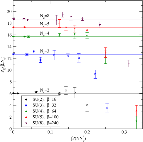
Figure 2: $P_{G}(\beta,N_{\rm c})$ as a function of the physical lattice size $\beta/(NN_{\rm c}^{2})$. Points denoted by open symbols are relatively low-statistics small volume simulations, included in order to illustrate the exponentially suppressed finite volume effects. These are omitted in the extrapolation. Finite-volume effects become visible when $\beta/(NN_{\rm c}^{2})\sim 0.2$. The points on the vertical axis indicate the infinite-volume estimate, obtained by fitting a constant to data in the range $\beta/(NN_{\rm c}^{2})<0.1$.

In Fig. 3 the effects arising from finite lattice spacing can be seen. We experience a qualitative change in the behavior of the plaquette expectation value at $\beta\approx N_{\rm c}^{2}$. The plaquette expectation value as a function of volume and lattice spacing $a$ is consistent with the assumption of correlation lengths being $\sim N_{\rm c}^{2}/\beta$.

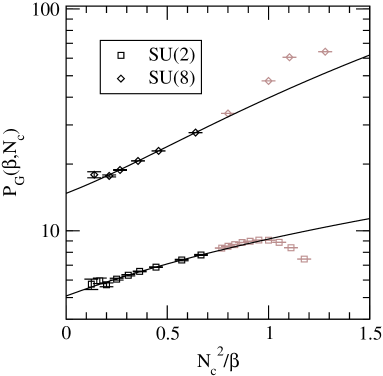
Figure 3: The solid line indicates the continuum extrapolation obtained by fitting a second order polynomial to the infinite-volume extrapolated data. Points denoted by lighter color are omitted. The bulk phase transition point is around $N_{\rm c}^{2}/\beta\sim 0.9$.

After numerous test runs we use in our simulations the requirement

$$N_{\rm c}^{2}<\beta\lesssim N(N_{\rm c}/3)^{2},$$ (3.3)

which is also the case in [11].

The continuum extrapolation is obtained by fitting a polynomial $P_{G}(N_{\rm c})=d_{1}+d_{2}/\beta+d_{3}\beta^{2}$ to the infinite-volume extrapolated data in Fig. 4 for each $N_{\rm c}$ separately. This functional form describes data quite well. The $\chi^{2}/$dof values for $N_{\rm c}=2,3,5$ are excellent but slightly discouraging for $N_{\rm c}=4,8$. The fitted values are show in Table 1. Using only statistical errors of the fitting parameters would underestimate the uncertainties of the continuum values, because the fit is dominated by points far from the continuum limit. Inclusion of higher order terms to the fitting function changes the continuum extrapolations by about one sigma. Therefore we expect that the 1-sigma error of the continuum extrapolated value is comparable to 2-sigma error of the fitting parameter $d_{1}$.

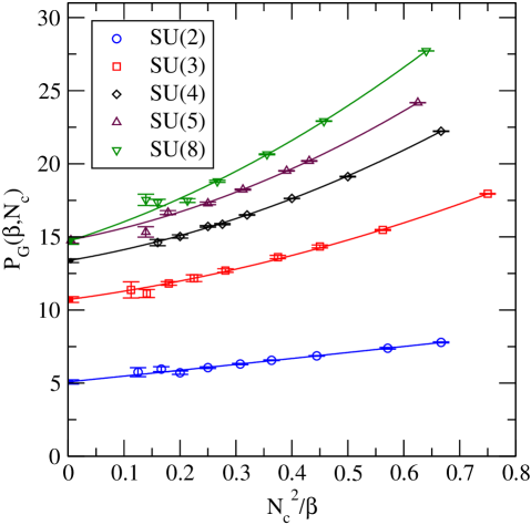
Figure 4: Continuum extrapolations of infinite-volume extrapolated data for each $N_{\rm c}$.

At the leading order in $N_{\rm c}$, our measurements agree with the prediction of planar diagram theory with $P_{G}(N_{\rm c},\infty)$, approaching a constant (Fig. 5). To study the next order contributions we fit polynomials $b_{1}+b_{2}/N_{\rm c}$, $b_{1}+b_{2}/N_{\rm c}+b_{3}/N_{\rm c}^{2}$ and $b_{1}+b_{3}/N_{\rm c}^{2}$ to the continuum extrapolated data in Fig. 6. We find that two last forms fit the data quite well. The $b_{2}$ coefficient is zero (within our resolution) as could be expected from the form of the perturbative coefficients, which are also functions of $N_{\rm c}^{2}$. The data is not accurate enough to determine higher order terms.

$N_{\rm c}$	fit					$\chi^{2}/$dof	$P_{G}(\infty,N_{\rm c})$
2	$5.09(15)$	$+$	$16(3)\beta^{-1}$	$+$	$3(11)\beta^{-2}$	$5.1/6$	5.1(3)
3	$10.7(2)$	$+$	$46(7)\beta^{-1}$	$+$	$4.85(6)\times 10^{2}\beta^{-2}$	$5.8/6$	10.7(4)
4	$13.38(13)$	$+$	$1.05(9)\times 10^{2}\beta^{-1}$	$+$	$2.58(14)\times 10^{3}\beta^{-2}$	$12.3/5$	13.4(3)
5	$14.8(2)$	$+$	$1.8(2)\times 10^{2}\beta^{-1}$	$+$	$7.9(5)\times 10^{3}\beta^{-2}$	$7.7/4$	14.8(4)
8	$14.7(2)$	$+$	$7.7(5)\times 10^{2}\beta^{-1}$	$+$	$5.3(3)\times 10^{4}\beta^{-2}$	$17.7/4$	14.7(4)

Table 1: The fitted values and $\chi^{2}/$dof of continuum extrapolations for each $N_{\rm c}$. The value in the brackets indicates the uncertainty of the last digit. The last column indicates the continuum limit with systematic errors included.

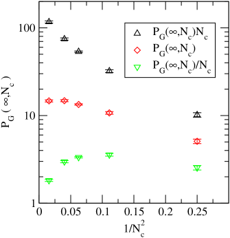
Figure 5: Comparing the leading order behavior of $P_{G}(\infty,N_{\rm c})$ in $N_{\rm c}$. As predicted by planar theory, $P_{G}$ approaches a constant in the large-$N_{\rm c}$ limit.

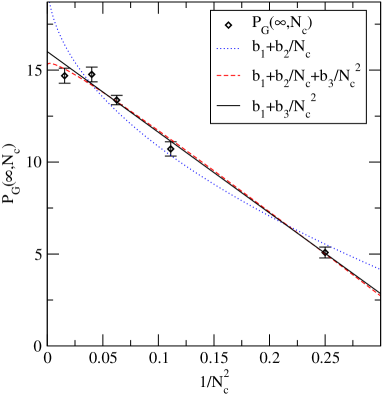
Figure 6: Comparing different fits for higher order terms in $N_{\rm c}$. The term $N_{\rm c}^{-1}$ is zero within our resolution implying that $P_{G}$ is a function of $N_{\rm c}^{-2}$.

As our final results we quote

$$B_{G}(N_{\rm c})+\left(\frac{43}{12}-\frac{157}{768}\pi^{2}\right)c_{4}^{\prime}=P_{G}(\infty,N_{\rm c})=15.9(2)-44(2)/N_{\rm c}^{2}$$ (3.4)

Inserting $N_{\rm c}=3$ we get

$$B_{G}(3)+\left(\frac{43}{12}-\frac{157}{768}\pi^{2}\right)c_{4}^{\prime}=11.0\pm 0.3,$$ (3.5)

which is consistent with the direct determination $10.7\pm 0.4$ [11].

function	values	$\chi^{2}/$dof
$b_{1}+b_{2}N_{\rm c}^{-1}$	$20.0(4)-28.9(12)N_{\rm c}^{-1}$	$27.9/3$
$b_{1}+b_{2}N_{\rm c}^{-1}+b_{3}N_{\rm c}^{-2}$	$15.25(11)+4.8(7)N_{\rm c}^{-1}-50.5(11)N_{\rm c}^{-2}$	$4.9/2$
$b_{1}+b_{3}N_{\rm c}^{-2}$	$15.9(2)-43.5(17)N_{\rm c}^{-2}$	$5.4/3$

Table 2: Different fitting functions for $P_{G}(\infty,N_{\rm c})$. The term $N_{\rm c}^{-1}$ provides a very bad description of the data (1st case) or has a coefficient consistent with zero within our resolution (2nd case); see also Fig. 6. The confidence values of fits are plausible for the last two functions.

4 Conclusions

The purpose of this paper has been to measure the $N_{\rm c}$-dependence of the expectation value of the plaquette in three-dimensional pure gauge theory. We have also outlined how the continuum $\overline{\rm{MS}}$ scheme free energy can be extracted from it. High precision lattice measurements of plaquette were performed with $N_{\rm c}=2,3,4,5$ and $8$ and the large-$N_{\rm c}$ limit was taken by extrapolation. We found that the non-perturbative input is $P_{G}=15.9(2)-44(2)/N_{\rm c}^{2}$. The data does not seem to allow for terms $\sim 1/N_{\rm c}$, and higher order terms, $\mathcal{O}(1/N_{\rm c}^{3})$ or $\mathcal{O}(1/N_{\rm c}^{4})$, are small enough such that the physical case $N_{\rm c}=3$ is very well described by this form.

Appendix A Tables

In this Appendix we collect the numerical results for the plaquette expectation value measurements, which have been used in the continuum extrapolations. The column $N_{\textrm{ind}}$ gives the number of independent measurements within a data set. The data sets used for SU(3) are the same as in [11].

SU(2) $\beta$ volume $N_{\textrm{ind}}$ $\langle 1-\frac{1}{N_{\rm c}}\textrm{Tr}[P]\rangle_{a}$ 6 $48^{3}$ 40719 0.1752161(16) 7 $48^{3}$ 42164 0.1488698(13) 9 $48^{3}$ 43187 0.1145493(10) 9 $320^{3}$ 5104 0.11454906(17) 11 $48^{3}$ 42993 0.0931322(8) 11 $320^{3}$ 8463 0.09313207(11) 13 $48^{3}$ 44195 0.0784776(7) 13 $320^{3}$ 8024 0.07847755(9) 16 $64^{3}$ 157777 0.06350205(19) 16 $320^{3}$ 14881 0.06350198(5) 20 $64^{3}$ 271054 0.05062861(11) 20 $320^{3}$ 12613 0.05062829(5) 24 $48^{3}$ 904993 0.04209730(8) 24 $64^{3}$ 317058 0.04209720(9) 24 $320^{3}$ 14961 0.04209733(4) 32 $64^{3}$ 868436 0.03148821(4) 32 $320^{3}$ 15064 0.03148828(2) 32 $400^{3}$ 6193 0.03148828(3)

SU(3) $\beta$ volume $N_{\textrm{ind}}$ $\langle 1-\frac{1}{N_{\rm c}}\textrm{Tr}[P]\rangle_{a}$ 12 $24^{3}$ 13459 0.2417125(8) 12 $32^{3}$ 10309 0.241717(6) 12 $48^{3}$ 16236 0.241714(3) 16 $24^{3}$ 15337 0.176526(6) 16 $32^{3}$ 18668 0.176531(3) 16 $48^{3}$ 19076 0.1765290(17) 16 $64^{3}$ 11833 0.1765302(14) 20 $24^{3}$ 11484 0.139295(5) 20 $32^{3}$ 11634 0.139283(3) 20 $48^{3}$ 19814 0.1392932(13) 24 $24^{3}$ 15992 0.115100(3) 24 $32^{3}$ 20983 0.1151000(19) 24 $48^{3}$ 20723 0.1150986(11) 24 $64^{3}$ 12101 0.1151009(9) 32 $48^{3}$ 20451 0.0854789(8) 32 $64^{3}$ 24662 0.0854815(5) 32 $96^{3}$ 24875 0.0854806(3) 40 $48^{3}$ 20817 0.0680065(6) 40 $64^{3}$ 25442 0.0680058(4) 40 $96^{3}$ 25700 0.06800677(19) 50 $64^{3}$ 33448 0.0541741(3) 50 $96^{3}$ 69213 0.05417428(10) 50 $128^{3}$ 29261 0.05417418(10) 50 $320^{3}$ 8298 0.05417406(5) 64 $96^{3}$ 25211 0.04217128(12) 64 $128^{3}$ 35565 0.04217113(6) 64 $320^{3}$ 7921 0.04217123(4) 80 $128^{3}$ 34310 0.03365240(6) 80 $320^{3}$ 8356 0.03365247(3)

SU(4) $\beta$ volume $N_{\textrm{ind}}$ $\langle 1-\frac{1}{N_{\rm c}}\textrm{Tr}[P]\rangle_{a}$ 24 $48^{3}$ 79254 0.2257701(7) 24 $64^{3}$ 15474 0.2257703(10) 32 $48^{3}$ 58752 0.1651322(6) 32 $64^{3}$ 16039 0.1651320(7) 40 $64^{3}$ 16704 0.1303851(5) 40 $96^{3}$ 33574 0.1303857(2) 40 $128^{3}$ 32872 0.13038581(13) 50 $64^{3}$ 17257 0.1033093(4) 50 $96^{3}$ 34295 0.10330876(16) 50 $128^{3}$ 33813 0.10330879(10) 58 $96^{3}$ 34810 0.08861313(14) 58 $128^{3}$ 33443 0.08861289(9) 64 $96^{3}$ 17342 0.08007684(17) 64 $128^{3}$ 50908 0.08007682(6) 80 $128^{3}$ 50664 0.06372001(5) 100 $128^{3}$ 51510 0.05076660(4)

SU(5) $\beta$ volume $N_{\textrm{ind}}$ $\langle 1-\frac{1}{N_{\rm c}}\textrm{Tr}[P]\rangle_{a}$ 40 $128^{3}$ 4667 0.2161236(5) 58 $128^{3}$ 8515 0.1447591(2) 64 $128^{3}$ 27137 0.13048507(12) 80 $128^{3}$ 22616 0.10336875(10) 100 $128^{3}$ 20238 0.08208926(8) 140 $128^{3}$ 12886 0.05817279(8) 140 $160^{3}$ 16049 0.05817267(5) 180 $128^{3}$ 12184 0.04505589(6) 180 $160^{3}$ 8597 0.04505586(5) SU(8) $\beta$ volume $N_{\textrm{ind}}$ $\langle 1-\frac{1}{N_{\rm c}}\textrm{Tr}[P]\rangle_{a}$ 100 $96^{3}$ 6493 0.2285506(5) 140 $96^{3}$ 9789 0.1584135(3) 180 $96^{3}$ 7127 0.1214678(2) 180 $128^{3}$ 3522 0.1214678(2) 240 $96^{3}$ 3755 0.0900746(3) 240 $128^{3}$ 3857 0.09007497(16) 300 $96^{3}$ 11266 0.07160377(11) 300 $128^{3}$ 3831 0.07160353(13) 400 $96^{3}$ 18120 0.05337892(6) 400 $128^{3}$ 4251 0.05337902(8) 460 $128^{3}$ 8656 0.04631022(5)

References

- [1] A. D. Linde, Infrared problem in thermodynamics of the Yang-Mills gas, Phys. Lett. B 96, 289 (1980).
- [2] D. J. Gross, R. D. Pisarski and L. G. Yaffe, QCD and instantons at finite temperature, Rev. Mod. Phys. 53, 43 (1981).
- [3] K. Kajantie, M. Laine, K. Rummukainen and Y. Schroder, The pressure of hot QCD up to g**6 ln(1/g), Phys. Rev. D 67, 105008 (2003) [hep-ph/0211321].
- [4] P. H. Ginsparg, First order and second order phase transitions in gauge theories at finite temperature, Nucl. Phys. B 170, 388 (1980). T. Appelquist and R. D. Pisarski, High-Temperature Yang-Mills theories and three-dimensional quantum chromodynamics, Phys. Rev. D 23, 2305 (1981).
- [5] K. Kajantie, M. Laine, K. Rummukainen and M. E. Shaposhnikov, Generic rules for high temperature dimensional reduction and their application to the standard model, Nucl. Phys. B 458, 90 (1996) [hep-ph/9508379].
- [6] E. Braaten and A. Nieto, Free energy of QCD at high temperature, Phys. Rev. D 53, 3421 (1996) [hep-ph/9510408].
- [7] K. Farakos, K. Kajantie, K. Rummukainen and M. E. Shaposhnikov, 3-d physics and the electroweak phase transition: A Framework for lattice Monte Carlo analysis, Nucl. Phys. B 442, 317 (1995) [hep-lat/9412091].
- [8] F. Di Renzo, A. Mantovi, V. Miccio and Y. Schroder, Four loop stochastic perturbation theory in 3d SU(3), Nucl. Phys. Proc. Suppl. 129, 590 (2004) [hep-lat/0309111]. 3-d lattice QCD free energy to four loops, JHEP 0405, 006 (2004) [hep-lat/0404003].
- [9] H. Panagopoulos, A. Skouroupathis and A. Tsapalis, Free energy and plaquette expectation value for gluons on the lattice, in three dimensions, Phys. Rev. D 73, 054511 (2006) [hep-lat/0601009].
- [10] F. Di Renzo, M. Laine, V. Miccio, Y. Schroder and C. Torrero, The leading non-perturbative coefficient in the weak-coupling expansion of hot QCD pressure, JHEP 0607, 026 (2006) [hep-ph/0605042].
- [11] A. Hietanen, K. Kajantie, M. Laine, K. Rummukainen and Y. Schroder, Plaquette expectation value and gluon condensate in three dimensions, JHEP 0501, 013 (2005) [hep-lat/0412008]. A. Hietanen, K. Kajantie, M. Laine, K. Rummukainen and Y. Schroder, Non-perturbative plaquette in 3d pure SU(3), PoS LAT2005, 174 (2006) [hep-lat/0509107].
- [12] G. ’t Hooft, A planar diagram theory for strong interactions, Nucl. Phys. B 72, 461 (1974).
-
[13]
B. Bringoltz and M. Teper,
The pressure of the SU(N) lattice gauge theory at large-N,
Phys. Lett. B 628, 113 (2005)
[hep-lat/0506034].
T. Eguchi and H. Kawai,
Reduction of dynamical degrees of freedom in the large N gauge theory,
Phys. Rev. Lett. 48, 1063 (1982).
H. B. Meyer,
The spectrum of SU(N) gauge theories in finite volume,
JHEP 0503 (2005) 064
[hep-lat/0412021].
H. B. Meyer,
Static forces in d = 2+1 SU(N) gauge theories,
[hep-lat/0607015].
R. Narayanan and H. Neuberger,
Large N gauge theories: Numerical results,
[hep-th/0607149]. M. Teper, Large-N gauge theories: Lattice perspectives and conjectures,
[hep-th/0412005]. - [14] C. P. Korthals Altes and H. B. Meyer, Hot QCD, k-strings and the adjoint monopole gas model, [hep-ph/0509018].
- [15] Y. Schroder, Tackling the infrared problem of thermal QCD, Nucl. Phys. Proc. Suppl. 129, 572 (2004) [hep-lat/0309112].
- [16] U. M. Heller and F. Karsch, One loop perturbative calculation of Wilson loops on finite lattices, Nucl. Phys. B 251, 254 (1985).
- [17] M. Laine and A. Rajantie, Lattice-continuum relations for 3d SU(N)+Higgs theories, Nucl. Phys. B 513 (1998) 471 [hep-lat/9705003].
- [18] A. D. Kennedy and B. J. Pendleton, Improved heat bath method for Monte Carlo calculations in lattice gauge theories, Phys. Lett. B 156, 393 (1985).
- [19] P. de Forcrand and O. Jahn, Monte Carlo overrelaxation for SU(N) gauge theories, [hep-lat/0503041].
- [20] M. J. Teper, SU(N) gauge theories in 2+1 dimensions, Phys. Rev. D 59 (1999) 014512 [hep-lat/9804008]. B. Lucini and M. Teper, SU(N) gauge theories in 2+1 dimensions: Further results, Phys. Rev. D 66 (2002) 097502 [hep-lat/0206027].