Leptonic widths of heavy quarkonia: QCD/NRQCD matching for the electromagnetic current at $O(\alpha_{s}v^{2})$

Abstract:

We construct the S-wave part of the electromagnetic vector annihilation current to $\mathcal{O}(\alpha_{s}v^{2})$, where $v$ is the non-relativistic quark velocity, for heavy quarks whose dynamics are described by the NRQCD action on the lattice. The NRQCD vector current for $Q\bar{Q}$ annihilation is expressed as a linear combination of lattice operators with quantum numbers $L=0$, $J^{P}=1^{-}$, and the coefficients are determined by matching to the corresponding continuum current in QCD to $\mathcal{O}(v^{2})$ at one-loop. The annihilation channel gives a complex amplitude with Coulomb-exchange and infrared singularities, making a careful choice for the contours of integration and infrared subtraction functions in the numerical integration necessary. An automated vertex generation program written in Python is employed, allowing us to use a realistic NRQCD action and an improved gluon lattice action; a change in the definition of either action is easily accommodated in this procedure. The final result is applicable to simulations of electromagnetic decays of heavy quarkonia, notably the $\Upsilon$ meson.

1 Introduction

Leptonic widths of heavy quarkonia such as the $\Upsilon$ or the $J/\psi$ are an important test of electroweak Standard Model in the heavy quark sector: The heavy quarks are the heaviest Standard Model particles and hence should be sensitive to possible new physics at or above the electroweak scale, and leptonic decays have experimentally clean signatures. Moreover, ratios of leptonic widths can be measured to good accuracy both experimentally and on the lattice.

The CLEO collaboration has experimental results to few-percent precision [1]:

$$\frac{\Gamma_{\Upsilon(2S)\to e^{+}e^{-}}}{\Gamma_{\Upsilon(1S)\to e^{+}e^{-}}}=0.457(6)$$ (1)

which has to be compared with the current best lattice result [2]

$$\frac{\Gamma_{\Upsilon(2S)\to e^{+}e^{-}}M^{2}_{\Upsilon(2S)}}{\Gamma_{\Upsilon(1S)\to e^{+}e^{-}}M^{2}_{\Upsilon(1S)}}=0.48(5)$$ (2)

There is thus a challenge to the lattice community to obtain a precision on theoretical predictions that can be compared to that achieved experimentally.

2 Matching S-wave decays between NRQCD and QCD

The leptonic width of a $\bar{Q}Q$ state is given by

$$\Gamma_{\bar{Q}Q\to l^{+}l^{-}}=\frac{8\pi}{3M_{\bar{Q}Q}}\left|\left<0\left|\mathbf{J}^{QCD}\right|\bar{Q}Q\right>\right|^{2}e_{Q}^{2}\alpha_{em}^{2}$$ (3)

with all the nonperturbative QCD contributions encapsulated in the matrix element $\left<0\left|\mathbf{J}^{QCD}\right|\bar{Q}Q\right>$. Unfortunately, it is not possible to simulate QCD with heavy quarks directly due to their short Compton wavelengths, so Non-Relativistic QCD (NRQCD) has to be used in lattice simulations of heavy quarkonia.

Hence, we need to match the desired QCD matrix element to a series of NRQCD matrix elements which can be measured on the lattice:

$$\left<0\left|\mathbf{J}^{QCD}\right|\bar{Q}Q\right>=\sum_{i}a_{i}\left<0\left|\mathbf{J}_{i}^{NRQCD}\right|\bar{Q}Q\right>$$ (4)

where the $a_{i}$ are the matching coefficients which we need to determine. For the case of S-wave decays, which we will study exclusively in this paper, we can take the NRQCD currents to be $\mathbf{J}_{i}^{NRQCD}={\bm{\sigma}}\left(\frac{\Delta^{2}}{M^{2}}\right)^{i}$.

To compute the matching coefficients perturbatively, we expand both the coefficients and the matrix elements perturbatively:

$$a_{i}=\sum_{n}\alpha_{s}^{n}a_{i}^{(n)}\hskip 56.9055pt\left<0\left|\mathbf{J}\right|\bar{Q}Q\right>=\sum_{n}\alpha_{s}^{n}\left<0\left|\mathbf{J}\right|\bar{Q}Q\right>^{(n)}$$ (5)

and match order by order in $\alpha_{s}$.

In the $\Upsilon$ system, the order of the NRQCD expansion parameters is $v^{2}\sim\alpha_{s}\sim 10\%$. Prima facie, this would suggest that to achieve $\sim 1\%$ accuracy, we would need to go to $\mathcal{O}(\alpha_{s}^{2},\alpha_{s}v^{2},v^{4})$. However, in matrix element ratios the $\mathcal{O}(\alpha_{s}^{2})$ terms cancel, and hence we only need to include $\mathcal{O}(\alpha_{s},\alpha_{s}v^{2},v^{4})$ corrections for $\sim 1\%$ accuracy.

If we are only interested in the ratio of leptonic widths of, say, $\Upsilon(2s)$ and $\Upsilon(1s)$, we do not care about the overall normalisation of the matrix element, and so for each decay we need only consider instead the quantity

$$\frac{M_{\textrm{ME}}}{a_{0}}=\left<J_{0}\right>+\frac{a_{1}}{a_{0}}\left<J_{1}\right>+\frac{a_{2}}{a_{0}}\left<J_{2}\right>\;.$$ (6)

and we can define matching coefficients for the ratio as

$$b_{1} \equiv \frac{a_{1}}{a_{0}}=\frac{a_{1}^{(0)}}{a_{0}^{(0)}}+\frac{\alpha_{s}}{a_{0}^{(0)}}\left[a_{1}^{(1)}-\frac{a_{1}^{(0)}a_{0}^{(1)}}{a_{0}^{(0)}}\right]\;,$$

$$b_{2} \equiv \frac{a_{2}}{a_{0}}=\frac{a_{2}^{(0)}}{a_{0}^{(0)}}\;.$$ (7)

In the following, we work in the Breit frame, where the decaying meson is stationary and the quark has momentum $p^{\mu}=(iE,0,0,Mv)$, use $v$ as the non-relativistic expansion parameter (which is exact at the order to which we are working) and treat the quarks as being exactly on-shell (which can also be shown to be justified).

3 The improved NRQCD action

The improved NRQCD action used for simulations is

$$\mathcal{S}_{NRQCD}=\sum_{x,t}\psi^{\dagger}\psi-\psi^{\dagger}\left(1-\frac{a\delta H}{2}\right)\left(1-\frac{aH_{0}}{2n}\right)^{n}U_{4}^{\dagger}\left(1-\frac{aH_{0}}{2n}\right)^{n}\left(1-\frac{a\delta H}{2}\right)\psi$$ (8)

with

$$aH_{0} = \frac{\Delta^{(2)}}{2M}$$

$$a\delta H = -c_{1}\,\frac{(\Delta^{(2)})^{2}}{8{(aM)}^{3}}+c_{2}\,\frac{i}{8{(aM)}^{2}}\left(\bm{\nabla}\cdot\tilde{\bm{E}}-\tilde{\bm{E}}\cdot\bm{\nabla}\right)-c_{3}\,\frac{1}{8{(aM)}^{2}}\bm{\sigma}\cdot(\tilde{\bm{\nabla}}\times\tilde{\bm{E}}-\tilde{\bm{E}}\times\tilde{\bm{\nabla}})$$

$$-c_{4}\,\frac{1}{2{(aM)}}\,\bm{\sigma}\cdot\tilde{\bm{B}}+c_{5}\,\frac{{\Delta^{(4)}}}{24{(aM)}}-c_{6}\,\frac{(\Delta^{(2)})^{2}}{16n{(aM)}^{2}}$$

where $n$ is a stability parameter for the euclidean-space Schrödinger equation, which must satisfy $n\geq 3/(Ma)$ for numerical stability. To the perturbative order considered here, we can take $c_{i}=1$.

As our glue action, we use a Symanzik improved action with tadpole improved links.

4 Automatically generating Feynman rules

In order to correctly determine the desired matching coefficients, we need to consider exactly the same NRQCD action in perturbation theory as is used in simulations. For the improved NRQCD action, the Feynman rules become extremely complicated: The QQg vertex, e.g., has $\sim 8,000$ terms, and the QQgg vertex has $\sim 70,000$ terms! It is clear that a traditional manual treatment would be extremely cumbersome and error-prone.

For this reason, we have developed HiPPy, an automated tool for generating Feynman rules from lattice actions. HiPPy is written entirely in Python with companion modules in Fortran 95, and is freely available from any of the authors. The main strength of HiPPy lies in its great flexibility: HiPPy is capable of handling not only various kinds of NRQCD actions, but also relativistic (staggered, Wilson …) quark and gluon actions with or without improvement. A description of HiPPy has been published in [3], and it is currently being used by HPQCD member to calculate a variety of different improvement and renormalisation constants. Due to its flexible design, a HiPPy-based program can easily accommodate a change in the quark or gluon action being used without the need for changes to the user code.

5 Matching at tree level

At tree-level, the relevant matrix elements are given by

$$\left<0\left|\mathbf{J}^{QCD}\right|\bar{Q}Q\right>^{(0)} = \bar{v}(-\mathbf{p}){\bm{\gamma}}u(\mathbf{p})=\chi^{\dagger}{\bm{\sigma}}\left(\frac{2}{3}+\frac{M}{3E}\right)\psi$$

$$\left<0\left|\mathbf{J}_{i}^{NRQCD}\right|\bar{Q}Q\right>^{(0)} = g_{i}(v)\chi^{\dagger}{\bm{\sigma}}\psi$$

where

$$g_{0}(v) = 1$$

$$g_{1}(v) = -\frac{4}{(Ma)^{2}}\sin^{2}\left(\frac{aMv}{2}\right)$$

$$g_{2}(v) = \frac{4}{(Ma)^{2}}\left[4\sin^{2}\left(\frac{aMv}{2}\right)-\sin^{2}(aMv)\right]$$

Expanding these matrix elements in powers of $v^{2}$, we determine $a_{i}^{(0)}$ to match:

$$a_{0}^{(0)}=1\;\;\;\;\;\;\;\;a_{1}^{(0)}=\frac{1}{6}\;\;\;\;\;\;\;\;a_{2}^{(0)}=\frac{1}{8}-\frac{(aM)^{2}}{72}$$ (9)

6 Matching to one-loop order

Expanding the matching condition to first order in $\alpha_{s}$ gives

$$\sum_{i}\underbrace{a_{i}^{(1)}}\limits_{\textrm{wanted}}\overbrace{\left<0\left|\mathbf{J}_{i}^{NRQCD}\right|\bar{Q}Q\right>^{(0)}}\limits^{\textrm{{known} functions of $v$}}=\underbrace{\left<0\left|\mathbf{J}^{QCD}\right|\bar{Q}Q\right>^{(1)}}\limits_{I_{QCD}}-\underbrace{\sum_{i}a_{i}^{(0)}\left<0\left|\mathbf{J}_{i}^{NRQCD}\right|\bar{Q}Q\right>^{(1)}}\limits_{I_{NRQCD}}$$ (10)

Both the QCD and the NRQCD matrix elements on the right-hand side contain odd powers of $v$ coming from the Coulomb-exchange singularity; however, only even powers of $v$ are available for matching on the left-hand side, so the odd powers must cancel exactly.

In fact, the odd powers of $v$ are a purely infrared phenomenon, and are known exactly:

$$I_{odd}=\frac{h(v)}{12v}=-\Im\left\{\frac{4}{3}\int\frac{d^{4}k}{(2\pi)^{4}}\frac{h(v)}{(\bm{k}^{2}+\mu^{2})(ik_{0}-\frac{\bm{k}^{2}+2\bm{k}\cdot\bm{p}}{2M})(ik_{0}+\frac{\bm{k}^{2}+2\bm{k}\cdot\bm{p}}{2M})}\right\}$$ (11)

where $h(v)$ is a known even function of $v$. We can hence analytically subtract the odd powers from both QCD and NRQCD by rearranging the right-hand side as

$$I_{QCD}-I_{NRQCD}=(I_{QCD}-I_{odd})-\left.(I_{NRQCD}-I_{odd})\right|_{\mathcal{B}}+\left.I_{odd}\right|_{\mathbf{R}^{4}\setminus\mathcal{B}}$$ (12)

where $\mathcal{B}$ signifies integration over the Brillouin zone only.

The term $(I_{QCD}-I_{odd})$ is known analytically, while the other terms are calculated numerically using farmed VEGAS on the CCHPCF SunFire Galaxy class computer.

The results obtained at various $v$ are then fitted with the ansatz

$$I_{QCD}-I_{NRQCD}=a_{0}^{(1)}-a_{1}^{(1)}g_{1}(v)$$ (13)

to obtain the matching coefficients at one-loop order.

6.1 The QCD form factors

The relevant QCD on-shell form factors

$$\left<0\left|\mathbf{J}^{QCD}\right|\bar{Q}Q\right>^{(1)} = F_{1,R}^{(1)}(4E^{2})\bar{v}(-\mathbf{p}){\bm{\gamma}}u(\mathbf{p})+F_{2}^{(1)}(4E^{2})\bar{v}(-\mathbf{p})\frac{\tilde{\mathbf{q}}}{2M}u(\mathbf{p})$$

$$= \Big{(}F_{1,R}^{(1)}(4E^{2})f_{1}(v^{2})+F_{2}^{(1)}(4E^{2})f_{2}(v^{2})\Big{)}\chi^{\dagger}{\bm{\sigma}}\psi$$

are simply the corresponding QED form factors (times a colour factor), which are well known at the one loop level. The $F_{2}$ term is both UV- and IR-finite; the $F_{1}$ term is UV-finite by virtue of the Ward identity, but IR divergences (which cancel against those in the NRQCD matrix elements) remain. Moreover, the $F_{1}$ term contains odd powers of $v$ which arise from the $1/v$ Coulomb-exchange singularity. As mentioned before, these odd powers are known to be the same in QCD and NRQCD, allowing them to be subtracted analytically.

6.2 The NRQCD self-energy

To account for the wavefunction renormalisation in NRQCD, as well as to establish the connection between the renormalised mass in terms of which the QCD form factors are formulated and the bare mass appearing in the NRQCD action, we need to compute the self-energy of the NRQCD heavy quarks.

The NRQCD self-energy, which is the sum of the usual “rainbow” and “tadpole” diagrams, can be decomposed as

$$a\Sigma(p_{0},\bm{p})=A+B(p_{0},\bm{p})\;aT(\bm{p})+C(p_{0},\bm{p})\left[1-e^{-iap_{0}}\left(1-aT(\bm{p})\right)\right]$$ (14)

where $T(\bm{p})$ is the tree-level kinetic energy, and from this form it is straightforward to derive the needed quantities, namely the wavefunction and (kinetic) mass renormalisation constants as

$$Z_{\psi}(\bm{p}) = 1+\alpha_{s}\left(a\Sigma+\frac{\partial a\Sigma}{\partial(iap_{0})}\right)_{\textrm{on-shell}}$$

$$Z_{M} = 1+\alpha_{s}2M\left.\frac{da\Sigma}{d\bm{p}^{2}}\right|_{\bm{p^{2}}=0}$$

Given the complicated nature of the Feynman rules, we employ automatic differentiation techniques [4] to calculate the derivatives.

6.3 The NRQCD vertex correction

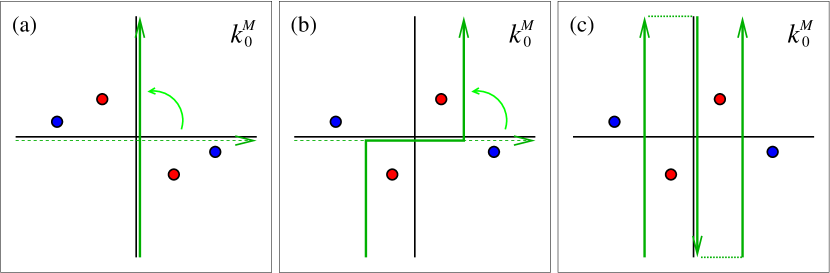
Figure 1: The position of the quark (red) and gluon (blue) poles in the Minkowskified energy plane. A normal Wick rotation (a) is only possible for $\mathbf{k}^{2}>-2\mathbf{p\cdot k}$; otherwise, the integration contour has to be deformed as in (b); for numerical work, the equivalent contour shown in (c) is adopted instead.

The NRQCD vertex correction suffers from the same infrared divergences that appear in the corresponding QCD diagram; we use a small gluon mass $\mu$ as an infrared regulator.

In terms of the Minkowskified energy variable $k_{0}^{M}$, the poles of the integrand (in the continuum limit) are at $\pm k_{0}^{M}=\sqrt{\mathbf{k}^{2}+\mu^{2}}-i\epsilon$ for the gluons, and $\pm k_{0}^{M}=\left(\frac{2\mathbf{p\cdot k}+\mathbf{k}^{2}}{2M}\right)-i\epsilon$ for the quarks, as shown in fig. 1. Hence, a normal Wick rotation between Euclidean and Minkowskian momenta is possible only for $\mathbf{k}^{2}>-2\mathbf{p\cdot k}$, since otherwise, the quark poles cross imaginary axis. We therefore need to deform the Euclidean contour of integration to avoid the quark poles and pick up the correct analytic continuation to Minkowksi space, and the choice of contour is shown in fig. 1 (c).

To subtract the odd powers of $v$ coming from the Coulomb-exchange singularity, we use the integral form of eqn. 11. The evaluation of the resulting finite integral is still quite hard numerically, and takes up the major part of the computer time used.

For $i>0$, the matrix elements of the NRQCD current $\mathbf{J}_{i}$ also contains tadpole-type diagrams. Since each tadpole loop reduces the $v$-dependence of the result by one power of $v^{2}$, this leads to a contamination of the lower-order matching coefficients by ”mixing down”, which would appear to necessitate a complete recalculation if higher-order currents are added in later. The solution lies in defining subtracted currents $\bar{J}_{i}=z_{ij}J_{j}^{NRQCD}$ where $z_{ij}$ is defined such that we have $\left<0\left|\bar{J}_{i}\right|\bar{Q}Q\right>^{(n)}=\mathcal{O}(v^{2i})$ for all $n$. For details, we have to refer the reader to [5].

7 Results

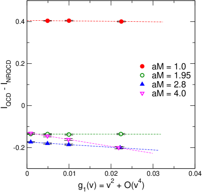
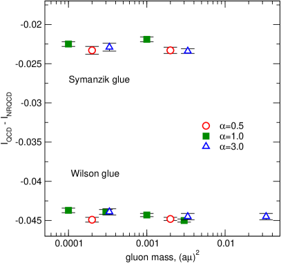
Figure 2: Left: the numerical results with the fit to extract the matching coefficients; right: a plot of results in different gauges against the infrared gluon mass, showing gauge and gluon mass independence.

$M_{0}a$	$n$	$a_{0}^{1}$	$a_{1}^{1}$	$b_{1}^{1}$	$b_{2}^{0}$
4.0	2	-0.1288(27)	-3.32(29)	-3.30(30)	-0.0972
2.8	2	-0.1732(21)	-1.35(22)	-1.32(22)	0.0161
1.95	2	-0.1358(16)	0.26(17)	0.14(17)	0.0722
1.0	4	0.4056(20)	-0.50(17)	-0.56(17)	0.1111

Table 1: The matching coefficients, as a function of the bare heavy quark mass, for the leptonic width ($a_{i}$) and leptonic width ratio ($b_{i}$). Note that $a_{0}^{(0)}=1$, $a_{1}^{(0)}=b_{1}^{(0)}=\frac{1}{6}$, and that there is no subtraction to prevent mixing down.

We have run our calculation at a number of different quark masses corresponding to the bottom quark on the MILC supercoarse, coarse and fine ensembles, and to the charm quark on the super-coarse ensemble. We have also performed extensive tests of gauge invariance, infrared regulator independence, and agreement with known results for $a_{0}^{(1)}$ at $v=0$ in the case of simpler NRQCD actions. A plot of our results can be seen in fig. 2, as can be a plot showing the gauge and regulator independence of our results. Our final results for the matching coefficients are given in tab. 1.

The authors thank G.P. Lepage and C.T.H. Davies for useful discussions and the Cambridge–Cranfield High Performance Computing Facility for advice and use of the SunFire supercomputer. This research was supported in part by the U.K. Royal Society, the Canadian Natural Sciences and Engineering Research Council (NSERC) and the Government of Saskatchewan.

References

• [1] CLEO Collaboration, J. L. Rosner et al., Phys. Rev. Lett. 96 (2006) 092003, [hep-ex/0512056].
• [2] A. Gray et al., Phys. Rev. D72 (2005) 094507, [hep-lat/0507013].
• [3] A. Hart, G. M. von Hippel, R. R. Horgan, and L. C. Storoni, J. Comput. Phys. 209 (2005) 340–353, [hep-lat/0411026].
• [4] G. M. von Hippel, Comput. Phys. Commun. 174 (2006) 569–576, [physics/0506222].
• [5] A. Hart, G. M. von Hippel, and R. R. Horgan, hep-lat/0605007.