Probing Nucleon Structure on the Lattice

Abstract

The QCDSF/UKQCD collaboration has an ongoing program to calculate nucleon matrix elements with two flavours of dynamical ${\cal O}(a)$ improved Wilson fermions. Here we present recent results on the electromagnetic form factors, the quark momentum fraction $\langle x\rangle$ and the first three moments of the nucleon’s spin-averaged and spin-dependent generalised parton distributions, including preliminary results with pion masses as low as 320 MeV.

1 Introduction

The ability of generalised parton distributions (GPDs) GPD to describe both exclusive and inclusive processes has led to an enormous amount of interest in these functions both experimentally and theoretically. Not only do GPDs encompass the ordinary electromagnetic form factors and parton distribution functions, but they also allow for the computation of the total quark contribution to the nucleon spin Ji as well as revealing important information on the transverse structure of the nucleon Diehl ; Bu . A full mapping of the parameter space spanned by GPDs is an extremely extensive task which needs support from non-perturbative techniques like lattice simulations.

Substantial progress has already been made in computing the first three moments of unpolarised, polarised QCDSF-1 ; MIT ; MIT-2 and tensor tensorGPDs GPDs on the lattice.

In this paper we present recent results from the QCDSF /UKQCD collaboration. In section 2 we investigate the $q^{2}$ dependence of the Dirac and Pauli electromagnetic form factors, while section 3 contains preliminary results for the average fraction of the nucleon’s momentum carried by the quarks, $\langle x\rangle$. Finally, in section 4 we present results for the first three moments of the GPDs $H$ and $\tilde{H}$.

2 Electromagnetic form factors

The study of the electromagnetic properties of hadrons provides important insights into the non-perturbative structure of QCD. The EM form factors reveal important information on the internal structure of hadrons including their size, charge distribution and magnetisation. Phenomenological interest in these form factors has been revived by recent Jefferson Lab polarisation experiments JLabFF measuring the ratio of the proton electric to magnetic form factors, $\mu^{(p)}G_{e}^{(p)}(q^{2})/G_{m}^{(p)}(q^{2})$. These experiments show that this ratio unexpectedly decreases almost linearly with increasing $q^{2}$, indicating that the proton’s electric form factor falls off faster than the magnetic form factor.

A lattice calculation of the $q^{2}$ dependence of the proton’s electromagnetic form factors can not only allow for a comparison with experiment, but also help in the understanding of the asymptotic behaviour of these form factors. Such a lattice calculation would also allow for the extraction of other phenomenologically interesting quantities such as magnetic and electric charge radii and magnetic moments.

2.1 Lattice Techniques

On the lattice, we determine the form factors $F_{1}(q^{2})$ and $F_{2}(q^{2})$ by calculating the following matrix element of the electromagnetic current

$$\langle p^{\prime},\,s^{\prime}|j_{\mu}|p,\,s\rangle = \bar{u}(p^{\prime},\,s^{\prime})\bigg{[}\gamma_{\mu}F_{1}(q^{2})$$ (1)

$$+\,i\sigma_{\mu\nu}\frac{q_{\nu}}{2m_{N}}F_{2}(q^{2})\bigg{]}u(p,\,s)\,,$$

where $u(p,\,s)$ is a Dirac spinor with momentum $p$ and spin polarisation $s$, $q=p^{\prime}-p$ is the momentum transfer with $Q^{2}=-q^{2}$, $m_{N}$ is the nucleon mass and $j_{\mu}$ is the electromagnetic current.

The form factors of the proton are obtained by using

$$j_{\mu}^{(p)}=\frac{2}{3}\bar{u}\gamma_{\mu}u-\frac{1}{3}\bar{d}\gamma_{\mu}d\ ,$$ (2)

while for iso-vector (i.e. proton $-$ neutron) form factors

$$j_{\mu}^{v}=\bar{u}\gamma_{\mu}u-\bar{d}\gamma_{\mu}d\ .$$ (3)

It is common to rewrite the form factors $F_{1}$ and $F_{2}$ as

$${\cal G}_{e}(q^{2}) = F_{1}(q^{2})+\frac{q^{2}}{(2m_{N})^{2}}F_{2}(q^{2}),$$ (4)

$${\cal G}_{m}(q^{2}) = F_{1}(q^{2})+F_{2}(q^{2}),$$ (5)

which are known as the electric and magnetic Sachs form factors, respectively.

At zero momentum transfer, $F_{1}(0)={\cal G}_{e}(0)$ gives the electric charge (e.g. 1 for the proton), while

$${\cal G}_{m}^{(p)}(0)=\mu^{(p)}=1+\kappa^{(p)}\ ,$$ (6)

gives the magnetic moment, where $F_{2}^{(p)}(0)=\kappa^{(p)}$ is the anomalous magnetic moment.

In order to extract the non-forward matrix elements from our lattice simulations, we compute ratios of three- and two-point functions

$${\cal R}(t,\tau;\vec{p}\,^{\prime},\vec{p};{\cal O})\,=\frac{C_{\Gamma}(t,\tau;\vec{p}\,^{\prime},\vec{p},{\cal O})}{C_{2}(t,\vec{p}\,^{\prime})}$$

$$\times\left[\frac{C_{2}(\tau,\vec{p}\,^{\prime})C_{2}(t,\vec{p}\,^{\prime})C_{2}(t-\tau,\vec{p}\,)}{C_{2}(\tau,\vec{p}\,)C_{2}(t,\vec{p}\,)C_{2}(t-\tau,\vec{p}\,^{\prime})}\right]^{\frac{1}{2}}$$

which for large time separations, $0\ll\tau\ll t\lesssim\frac{1}{2}L_{T}$, where $L_{T}$ is the temporal extent of our lattice, is proportional to the matrix element we are interested in, $\langle p^{\prime}|{\cal O}_{q}|p\rangle$. The nucleon two- and three-point functions are given, respectively, by

$$C_{2}(\tau,\vec{p}) = {\rm Tr}\left[\Gamma_{\rm unpol}\langle B(\tau,\vec{p})\overline{B}(0,\vec{p})\rangle\right]\,,$$

$$C_{\Gamma}(t,\tau;\vec{p}\,^{\prime},\vec{p},{\cal O}) = {\rm Tr}\left[\Gamma\langle B(t,\vec{p}\,^{\prime}){\cal O}(\tau)\overline{B}(0,\vec{p})\rangle\right]\,.$$ (8)

Here $t$ and $\tau$ are the Euclidean times of the nucleon sink and operator insertion, respectively, $\vec{p}\,^{\prime}\ (\vec{p})$ is the nucleon momentum at the sink (source), and ${\cal O}$ is the local vector current

$${\cal O}(\tau)=\psi(\tau)\gamma_{\mu}\psi(\tau)\ ,$$ (9)

which we renormalise non-perturbatively Bakeyev:2003ff . The trace in Eq. (8) is over spinor indices and the $\Gamma$ matrix determines the polarisation of the nucleon with $\Gamma_{\text{unpol}}=\frac{1}{2}(1+\gamma_{4})$. We note here that in the calculation of nucleon matrix elements, we neglect contributions coming from disconnected quark diagrams as these are extremely computationally demanding. Hence, in the following we mainly restrict ourselves to the calculation of iso-vector matrix elements where the disconnected quark contributions cancel.

Finally, we use the Sommer parameter, $r_{0}$, to set the scale with $r_{0}=0.5$ fm.

2.2 Results

Of particular interest is the need to understand the behaviour of the form factor $F_{2}(Q^{2})$. The question arises which is the best way to fit the form factor since such a fitting function also allows an extrapolation of the form factor to $Q^{2}=0$. This is a necessary ingredient to find the anomalous magnetic moment of the nucleon, $\kappa$.

Based on perturbative QCD, $F_{1}$ should scale asymptotically as $1/Q^{4}$, while $F_{2}\sim 1/Q^{6}$ Brodsky:1974vy ; Lepage:1980fj . It is difficult to obtain lattice data with high enough precision over a large enough range of $Q^{2}$ values to distinguish between a dipole or tripole behaviour. It may, however, be instructive to consider the form factor ratio $F_{2}(Q^{2})/F_{1}(Q^{2})$ since asymptotically this ratio should scale as $1/Q^{2}$. Spin polarisation experiments have instead found that the data is compatible with

$$\frac{F_{2}(Q^{2})}{F_{1}(Q^{2})}\sim\frac{1}{\sqrt{Q^{2}}}\ .$$ (10)

To investigate the asymptotic behaviour of the form factor ratio $F_{2}(Q^{2})/F_{1}(Q^{2})$, we plot in Fig. 1 the results for $\sqrt{Q^{2}}F_{2}/F_{1}$ obtained at three working points with approximately the same pion mass, but with different values of the lattice spacing. Here we observe the lattice data to be consistent with a constant for $Q^{2}>1.5\,\text{GeV}^{2}$, similar to the experimental data. Multiplying these results by an extra factor of $\sqrt{Q^{2}}$, as suggested by perturbative QCD, would clearly destroy the plateau. Quantitatively, though, the lattice data is higher than the corresponding experimental ratios, cf Belitsky:2002kj . This shows that the lattice simulations are able to reproduce the qualitative features of the experimental data, but for a quantitative reproduction the pion mass is still unrealistically large.

In the following we fit $F_{1}$ and $F_{2}$ with a dipole ansatz

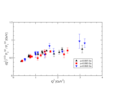
Figure 1: $\sqrt{Q^{2}}\,F_{2}/F_{1}$ form factor ratio on three datasets with the same pion mass ($\approx 550$ MeV), but with different lattice spacings, $a=0.085,\,0.080,\,0.068$ fm.

$$F_{i}^{(v)}(q^{2})=\frac{F_{i}(0)}{(1-q^{2}/M_{i}^{2})^{2}}$$ (11)

where $F_{1}^{(v)}(0)=1$, $F_{2}^{(v)}(0)=\kappa^{(v)}$ and $M_{i}$ is the fitted dipole mass for the form factor, $i$.

We display our results for the isovector magnetic moment in Fig. 2 as a function of $m_{\pi}^{2}$. Our results are in good agreement with recent quenched Gockeler:2003ay ; Boinepalli:2006xd ; Alexandrou:2006ru and $N_{f}=2$ Alexandrou:2006ru results, which indicates that there appears to be little effect due to quenching on the magnetic moments, as predicted in Young:2004tb . The experimental value is indicated by a star at the physical pion mass. We clearly see that a linear extrapolation would miss the experimental point. This, however, is not completely unexpected as results from chiral perturbation theory suggest that we should observe a dramatic increase in the results at lighter pion masses Gockeler:2003ay ; Young:2004tb . The new points at lighter pion masses, $m_{\pi}^{2}<0.2$ GeV², are beginning to show a hint of such curvature, although more work needs to be done to reduce the error bars.

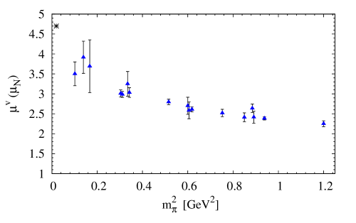
Figure 2: Results for the isovector magnetic moment as a function of $m_{\pi}^{2}$. The experimental value is denoted by the star.

3 Quark momentum fraction, $\langle x\rangle$

Forward matrix elements (no momentum transfer) provide moments of quark distributions in some scheme, $\cal S$, at some scale, $M$:

$$\langle N(\vec{p})|{\cal O}^{\{\mu_{1}\cdots\mu_{n}\}}_{q}|N(\vec{p})\rangle^{\cal S}=2v_{n}^{(q){\cal S}}(g^{\cal S}(M))\;p^{\mu_{1}}\cdots p^{\mu_{n}},$$ (12)

where

$${\cal O}_{q}^{\{\mu_{1}\cdots\mu_{n}\}}=\overline{q}\,i^{n-1}\,\gamma^{\{\mu_{1}}\,\overset{\leftrightarrow}{D}^{\mu_{2}}\cdots\overset{\leftrightarrow}{D}^{\mu_{n}\}}\!q\ ,$$ (13)

$\overset{\leftrightarrow}{D}=\frac{1}{2}(\overset{\rightarrow}{D}-\overset{\leftarrow}{D})$ and $\{\cdots\}$ indicates symmetrisation of indices and removal of traces.

Matrix elements with no momentum transfer are determined from a simplified version of the ratio of three-point to two-point correlation functions given in Eq. (2.1). See Gockeler:2004wp for additional details.

We use non-perturbative renormalisation as outlined in Section 5.2.3 of Gockeler:2004wp to convert our lattice results to the $\overline{\text{MS}}$ scheme at $\mu^{2}=4$ GeV².

In the language of the parton model, $v_{n}^{q}$ is often denoted by $\langle x^{n-1}\rangle^{q}$

$$\langle x^{n-1}\rangle^{q}=\int^{1}_{0}\,dx\,x^{n-1}\,[q(x)+(-1)^{n}\bar{q}(x)]=v_{n}^{q}\ .$$ (14)

Of particular interest is the first ($n=2$) moment, $v_{2}^{q}=\langle x\rangle^{q}$, which determines the fraction of the nucleon’s momentum carried by the quark, $q$. This quantity is notorious on the lattice for producing values much larger than phenominologically accepted results. These discrepancies can possibly be explained by the fact that all lattice calculations to date have been performed at quark masses that are much larger than the physical masses Detmold:2001jb . Hence, it is a challenge for current lattice simulations to calculate $\langle x\rangle$ at small enough quark masses in order to search for the severe curvature predicted in Ref. Detmold:2001jb .

Figure 3 displays preliminary results for $\langle x\rangle^{(u-d)}$ with pion masses as low as $\sim 320$ MeV. Before we can draw any conclusions on the behaviour at small quark masses, we need to study scaling violations and finite size effects more carefully. Indeed, it has been suggested Detmold:2005pt ; Detmold:2003rq that a volume of at least (4 fm)³ is required to confirm the predicted chiral curvature.

Figure 3: Isovector $\langle x\rangle$ as a function of $m_{\pi}^{2}$ in the $\overline{\text{MS}}$ scheme at $\mu^{2}=4$ GeV². These preliminary results are obtained at four different lattice spacings (in fm): 0.092 (triangles), 0.085 (diamonds), 0.080 (circles) and 0.068 (squares). The star indicates the phenomenological result of the MRST analysis Martin:2001es as given in Gockeler:2004wp . This is in agreement with a recent higher order analysis Blumlein:2006be .

4 Generalised parton distributions

4.1 Matrix Elements And Moments of GPDs

For a lattice calculation of GPDs, we work in Mellin-space to relate matrix elements of local operators to Mellin moments of the GPDs. The non-forward matrix elements of the twist-2 operator in Eq. (13) specifies the $(n-1)^{th}$ moments of the spin-averaged generalised parton distributions. Replacing $\gamma$ with $\gamma_{5}\gamma$ leads to moments of the spin-dependent GPDs. In particular, for the unpolarised GPDs, we have

$$\!\!\int_{-1}^{1}dx\,x^{n-1}\,H^{q}(x,\xi,t)=H^{q}_{n}(\xi,t)\,,\!\int_{-1}^{1}dx\,x^{n-1}\,E^{q}=E^{q}_{n}\,,$$ (15)

where Ji

$$H^{q}_{n}(\xi,t) = \sum_{i=0}^{\lfloor\frac{n-1}{2}\rfloor}A^{q}_{n,2i}(t)(-2\xi)^{2i}+C^{q}_{n}(t)(-2\xi)^{n}|_{n\text{ even}}\,,$$

$$E^{q}_{n}(\xi,t) = \sum_{i=0}^{\lfloor\frac{n-1}{2}\rfloor}B^{q}_{n,2i}(t)(-2\xi)^{2i}-C^{q}_{n}(t)(-2\xi)^{n}|_{n\text{ even}}\,.$$

Here we denote the invariant of the momentum transfer by $t=\Delta^{2}=(p^{\prime}-p)^{2}$. The generalised form factors $A^{q}_{n,2i}(t)$, $B^{q}_{n,2i}(t)$ and $C^{q}_{n}(t)$ for the lowest three moments are extracted from non-forward nucleon matrix elements of the operators in Eq. (13) MIT .

For the lowest moment, $A_{10}$ and $B_{10}$ are just the Dirac and Pauli form factors $F_{1}$ and $F_{2}$, respectively

$$\int_{-1}^{1}dx\,H^{q}(x,\xi,t) = A^{q}_{10}(t)=F_{1}(t)\,,$$ (17)

$$\int_{-1}^{1}dx\,E^{q}(x,\xi,t) = B^{q}_{10}(t)=F_{2}(t)\,,$$ (18)

while $\widetilde{A}_{10}$ and $\widetilde{B}_{10}$ are the usual axial-vector and pseudoscalar form factors, respectively

$$\int_{-1}^{1}dx\,\widetilde{H}^{q}(x,\xi,t) = \widetilde{A}^{q}_{10}(t)=g_{A}(t)\,,$$ (19)

$$\int_{-1}^{1}dx\,\widetilde{E}^{q}(x,\xi,t) = \widetilde{B}^{q}_{10}(t)=g_{P}(t)\,.$$ (20)

We also observe that in the forward limit ($t=\xi=0$), the moments of $H_{q}$ reduce to the moments of the unpolarised parton distribution $A_{n0}(0)=\langle x^{n-1}\rangle$.

4.2 Results For Generalised Form Factors

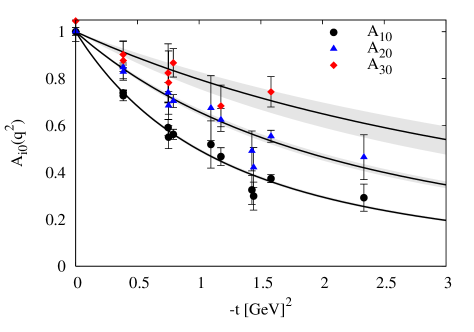
Figure 4: Generalised form factors $A^{u-d}_{10},\ A^{u-d}_{20}$, $A^{u-d}_{30}$ together with a dipole fit. All form factors have been normalised to unity.

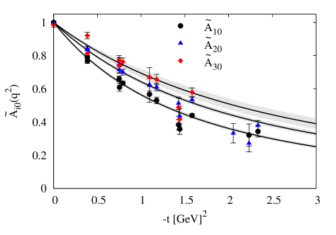
Figure 5: Generalised form factors $\widetilde{A}^{u-d}_{10},\ \widetilde{A}^{u-d}_{20}$, $\widetilde{A}^{u-d}_{30}$ together with a dipole fit. All form factors have been normalised to unity.

Burkardt Bu has shown that the spin-independent and spin-dependent generalised parton distributions $H(x,0,t)$ and $\widetilde{H}(x,0,t)$ gain a probability interpretation when Four-ier transformed to impact parameter space at longitudinal momentum transfer $\xi=0$

$$q(x,\vec{b}_{\perp})=\int\frac{d^{2}\Delta_{\perp}}{(2\pi)^{2}}\,{\rm e}^{-i\vec{b}_{\perp}\cdot\vec{\Delta}_{\perp}}H(x,0,-\Delta_{\perp}^{2})\,,$$ (21)

(and similar for the polarised $\Delta q(x,\vec{b}_{\perp})$) where $q(x,\vec{b}_{\perp})$ is the probability density for a quark with longitudinal momentum fraction $x$ and at transverse position (or impact parameter) $\vec{b}_{\perp}$.

Burkardt Bu also argued that $H(x,0,-\Delta_{\perp}^{2})$ becomes $\Delta_{\perp}^{2}$-independent as $x\rightarrow 1$ since, physically, we expect the transverse size of the nucleon to decrease as $x$ increases, i.e. $\lim_{x\rightarrow 1}q(x,\vec{b}_{\perp})\propto\delta^{2}(\vec{b}_{\perp})$. As a result, we expect the slopes of the moments of $H(x,0,-\Delta_{\perp}^{2})$ in $\Delta_{\perp}^{2}$ to decrease as we proceed to higher moments. This is also true for the polarised moments of $\widetilde{H}(x,0,-\Delta_{\perp}^{2})$, so from Eq. (LABEL:GPDmoments) with $\xi=0$, we expect that the slopes of the generalised form factors $A_{n0}(t)$ and $\widetilde{A}_{n0}(t)$ should decrease with increasing $n$.

In Figs. 4 and 5, we show the $t$-dependence of $A_{n0}(t)$ and $\widetilde{A}_{n0}(t)$, respectively, $n=1,2,3$, for $\beta=5.40$, $\kappa_{\text{sea}}=\kappa_{\text{val}}=0.13500$. The form factors have been normalised to unity to make a comparison of the slopes easier and we fit the form factors with a dipole form as in Eq. (11). We observe here that the form factors for the unpolarised moments are well separated and that their slopes do indeed decrease with increasing $n$ as predicted. For the polarised moments, we observe a similar scenario, however here the change in slope between the form factors is not as large. The flattening of the GFFs $A_{n0}(t)$ has first been observed in Ref. MIT-2 , where at the same time practically no change in slope was seen going from $\widetilde{A}_{20}(t)$ to $\widetilde{A}_{30}(t)$.

Although fitting the form factors with a dipole is purely phenomenological (see Ref. Diehl:2004cx for an alternative ansatz), it does provide us with a useful means to measure the change in slope of the form factors by monitoring the extracted dipole masses as we proceed to higher moments. We have calculated these generalised form factors on a subset of our full complement of $(\beta,\,\kappa)$ combinations and have extracted the corresponding dipole masses. Recall that $A_{10}$ is the Dirac form factor $F_{1}$, while $\tilde{A}_{10}$ is the axial form factor $g_{A}$. Hence the dipole fits can be compared with experiment. A linear extrapolation produces a result larger than experiment for both the polarised and unpolarised case, although the findings of Ref. Thomas suggest that the chiral extrapolation of the dipole masses of the electromagnetic form factors may be non-linear.

In Fig. 6 we show the lowest three moments of the GPD $H(x,\xi=0,t)$ (top) and $\widetilde{H}(x,\xi=0,t)$ (bottom) in impact parameter space. The curves correspond to the Fourier-transformation of our dipole ansatz Eq. (11), with the dipole masses extrapolated linearly to the chiral limit, to $b_{\perp}$-space, and the shaded error band is a result of the errors in the extrapolated dipole masses at the physical pion mass. The curves have been normalised so that they represent line densities with $\int{\rm d}b\,q^{n}(b)=1$. The top figure of Fig. 6 clearly shows how the $u-d$ quark distribution narrows as we proceed to higher moments $n$ and thereby larger values of the average momentum fraction, while for the polarised case in the bottom figure, the narrowing of the distribution is not so severe.

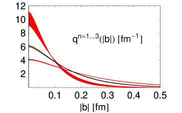
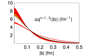
Figure 6: The lowest three moments of the GPD $H(x,\xi=0,t)$ (top) and $\widetilde{H}(x,\xi=0,t)$ (bottom) in impact parameter space as a function of impact parameter, $b$.

References

- (1) D. Müller et al., Fortsch. Phys. 42 (1994) 101 [hep-ph/9812448]; A. V. Radyushkin, Phys. Rev. D 56 (1997) 5524 [hep-ph/9704207]; M. Diehl et al., Phys. Lett. B 411 (1997) 193 [hep-ph/9706344].
- (2) X. D. Ji, Phys. Rev. Lett. 78 (1997) 610 [hep-ph/9603249]; X. D. Ji, J. Phys. G 24 (1998) 1181 [hep-ph/9807358].
- (3) M. Diehl, Eur. Phys. J. C 25 (2002) 223 [Erratum-ibid. C 31 (2003) 277] [hep-ph/0205208].
- (4) M. Burkardt, Int. J. Mod. Phys. A 18 (2003) 173 [hep-ph/0207047].
- (5) M. Göckeler et al., Phys. Rev. Lett. 92 (2004) 042002, [hep-ph/0304249]; Nucl. Phys. Proc. Suppl. 128 (2004) 203, [hep-ph/0312104]; Nucl. Phys. Proc. Suppl. 140 (2005) 399, [hep-lat/0409162]; Few Body Syst. 36 (2005) 111 [hep-lat/0410023].
- (6) Ph. Hägler et al., Phys. Rev. D 68 (2003) 034505 [hep-lat/0304018].
- (7) Ph. Hägler et al., Phys. Rev. Lett. 93 (2004) 112001, [hep-lat/0312014]; J. W. Negele et al., Nucl. Phys. Proc. Suppl. 128 (2004) 170 [hep-lat/0404005]; Ph. Hägler et al., Eur. Phys. J. A 24S1 (2005) 29 [hep-ph/0410017]; R. G. Edwards et al., PoS LAT2005 (2006) 056 [hep-lat/0509185].
- (8) M. Göckeler et al., Nucl. Phys. A 755 (2005) 537 [hep-lat/0501029]; M. Göckeler et al., Phys. Lett. B 627 (2005) 113 [hep-lat/0507001]; M. Göckeler et al., Nucl. Phys. Proc. Suppl. 153 (2006) 146 [hep-lat/0512011]; M. Diehl et al., hep-ph/0511032.
- (9) M. K. Jones et al., Phys. Rev. Lett. 84 (2000) 1398 [nucl-ex/9910005]; O. Gayou et al., Phys. Rev. C 64 (2001) 038202; O. Gayou et al., Phys. Rev. Lett. 88 (2002) 092301 [nucl-ex/0111010].
- (10) T. Bakeyev et al., Phys. Lett. B 580 (2004) 197 [hep-lat/0305014].
- (11) S. J. Brodsky and G. R. Farrar, Phys. Rev. D 11 (1975) 1309.
- (12) G. P. Lepage and S. J. Brodsky, Phys. Rev. D 22 (1980) 2157.
- (13) A. V. Belitsky et al., Phys. Rev. Lett. 91 (2003) 092003 [hep-ph/0212351].
- (14) M. Göckeler et al., Phys. Rev. D 71 (2005) 034508 [hep-lat/0303019].
- (15) S. Boinepalli et al., hep-lat/0604022.
- (16) C. Alexandrou et al., Phys. Rev. D 74 (2006) 034508 [hep-lat/0605017].
- (17) R. D. Young et al., Phys. Rev. D 71 (2005) 014001 [hep-lat/0406001].
- (18) M. Göckeler et al., Phys. Rev. D 71 (2005) 114511 [hep-ph/0410187].
- (19) W. Detmold et al., Phys. Rev. Lett. 87 (2001) 172001 [hep-lat/0103006].
- (20) A. D. Martin et al., Eur. Phys. J. C 23 (2002) 73 [hep-ph/0110215].
- (21) J. Blumlein et al., hep-ph/0607200.
- (22) W. Detmold and C. J. Lin, Phys. Rev. D 71 (2005) 054510 [hep-lat/0501007].
- (23) W. Detmold et al., Mod. Phys. Lett. A 18 (2003) 2681 [hep-lat/0310003].
- (24) M. Diehl et al., Eur. Phys. J. C 39 (2005) 1 [hep-ph/0408173].
- (25) J. D. Ashley et al., Eur. Phys. J. A 19 (2004) 9 [hep-lat/0308024].
- (26) C. R. Allton et al.,Phys. Rev. D 65 (2002) 054502 [hep-lat/0107021].