Quark condensate in two-flavor QCD

Abstract

We compute the condensate in QCD with two flavors of dynamical fermions using numerical simulation. The simulations use overlap fermions, and the condensate is extracted by fitting the distribution of low lying eigenvalues of the Dirac operator in sectors of fixed topological charge to the predictions of Random Matrix Theory.

I Introduction

The quark condensate $\Sigma=\langle 0|\bar{q}q|0\rangle$ is the order parameter associated with the spontaneous breaking of chiral symmetry in QCD. Along with the pseudoscalar decay constant, it is one of the two fundamental parameters of the lowest order chiral Lagrangian which is the low energy effective field theory for QCD. As such, its value is an interesting physical quantity whose determination presents a challenge to lattice QCD methodology. While there have been many calculations of $\Sigma$ in quenched QCD, results for QCD with dynamical fermions are relatively sparse (for a summary of recent results, see Ref. McNeile:2005pd ). This paper is a computation of $\Sigma$ for QCD with two flavors of dynamical overlap fermionsNeuberger:1997fp ; Neuberger:1998my . Overlap fermions implement chiral symmetry exactly at nonzero lattice spacing via the Ginsparg-WilsonGinsparg:1981bj relation. This paper is an extension of our earlier work published in Ref. DeGrand:2005vb , which was primarily about algorithms, and Ref. DeGrand:2006uy , where we use the same methodology to extract $\Sigma$ in $N_{f}=1$ QCD.

Rather than measure $\langle\bar{q}q\rangle$ directly, we will determine the particular combination of the coefficients of the low energy effective field theory, $\Sigma=f^{2}B$, in the usual parameterization

$${\cal L}_{2}=\frac{f^{2}}{4}{\rm Tr}(\partial_{\mu}U\partial_{\mu}U^{\dagger})+B\frac{f^{2}}{2}{\rm Tr}[M(U+U^{\dagger})].$$ (1)

One expects that the quantity $\langle\overline{q}q\rangle$ (as computed, for example, in a lattice simulation at some quark mass $m_{q}$ and simulation volume $V$) is a function of $\Sigma$, $f$, $m_{q}$, and $V$. For the remainder of this paper, we will refer to the quantity $\Sigma$ as the condensate, and this is the quantity we will compute on the lattice.

This is done using the low-lying eigenvalues of the QCD Dirac operator in a finite volume, whose distribution can be predicted by random matrix theory (RMT) Shuryak:1992pi ; Verbaarschot:1993pm ; Verbaarschot:1994qf . This hypothesis has been checked extensively by lattice calculations, mainly in quenched simulations Berbenni-Bitsch:1997tx ; Damgaard:1998ie ; Gockeler:1998jj ; Edwards:1999ra ; Giusti:2003gf ; Follana:2005km ; Wennekers:2005wa , but also in dynamical ones using staggered quarks Berbenni-Bitsch:1998sy ; Damgaard:2000qt . Our analysis is based on the distribution of the $k$-th eigenvalue from RMT as presented in Refs. Damgaard:2000ah ; Damgaard:2000qt . The prediction is for the distribution of the $k$-th eigenvalue of the Dirac operator, $\lambda_{k}$, in each topological sector, which is a function of the dimensionless quantity $\zeta=\lambda_{k}\Sigma V$, where $\Sigma$ is the chiral condensate and $V$ is the volume of the box. These distributions are universal and depend only on the number of flavors and the topological charge. They depend parametrically on the dimensionless quantity $m_{q}\Sigma V$. By comparing the distribution of the eigenvalues with the RMT prediction one can thus measure the chiral condensate $\Sigma$. This method gives the zero quark mass, infinite volume condensate directly.

The validity of the approach can be verified by comparing the shape of the distribution for the various modes and topological sectors. A too small volume causes deviations in the shape, particularly for the higher modes. Two recent large scale studies using the overlap operator on quenched configurations Bietenholz:2003mi ; Giusti:2003gf , found that with a length larger than $1.2~{}{\rm fm}$ and $1.5~{}{\rm fm}$ respectively, the RMT predictions match the result of the simulation. Our dynamical lattices have a spatial extent of about 1.5 fm and we have a smaller volume from our earlier work. As we will see, random matrix theory describes our data quite well.

The RMT predictions are made with the assumption that the volume is infinite. In the epsilon-regime of chiral perturbation theory, finite volume modifies the formula for the condensate by multiplication by a shape factor, $a^{3}\Sigma\rightarrow\rho a^{3}\Sigma$, where

$$\rho=1+\frac{N_{f}^{2}-1}{N_{f}}\frac{c(l_{i}/l)}{f_{\pi}^{2}L^{2}}$$ (2)

and $c(l_{i}/l)$ depends on the geometryGasser:1986vb . (It is 0.1405 for hypercubes.) We do not know $\rho$ since we have not measured $f_{\pi}$, but combining our lattice spacing and lattice size with $f_{\pi}=93$ MeV, we expect $\rho\sim 1.42$ for our simulations. In what follows, we will refer to the quantity we extract from RMT fits as $\Sigma$ rather than the more proper label of $\rho\Sigma$. Ignoring $\rho$ introduces a systematic uncertainty into our result.

The lattice calculation has four parts: The first is the algorithm. Our calculations are performed with overlap fermions, which possess exact chiral symmetry at nonzero lattice spacing. A variation on the standard Hybrid Monte Carlo allows us to perform simulations in sectors of fixed topologyBode:1999dd ; Cundy:2005mr ; ouralg . We review the algorithm in Sec. II.1.

The extraction of $\Sigma$ from a fit to the eigenvalues of the Dirac operator is described in Sec. II.2.

Next, we need a lattice spacing to convert the dimensionless lattice-regulated condensate to a dimensionful number. We obtain the lattice spacing through the Sommer parameter from the static quark potentialSommer:1993ce . This is described in Sec. II.3.

Finally, we need a matching factor, to convert the lattice-regulated condensate to its $\overline{MS}$ value. We do this using the Regularization Independent schemeMartinelli:1994ty . This is described in Sec. II.4.

To anticipate our results, which are summarized in Sec. III, the larger simulation volume considerably improves the quality of the RMT fits. The value of the lattice-regulated condensate we obtain here is quite consistent with our earlier result. We find, however, that the nonperturbative matching factor we determine is quite different from the perturbative matching factor used in Ref. DeGrand:2005vb . Our final answer is $\Sigma^{1/3}=282(10)$ MeV; the quoted error is statistical (from the simulation); in addition, we estimate that this number exceeds the true result by a systematic factor $\rho^{1/3}=1.13$.

II Methodology

II.1 Lattice action and simulation algorithm

The massless overlapNeuberger:1997fp ; Neuberger:1998my operator is

$$D=D_{ov}(m=0)=R_{0}\left[1+\gamma_{5}\epsilon(h(-R_{0}))\right]$$ (3)

where $\epsilon(h)=h/\sqrt{h^{2}}$ is the sign function of the Hermitian kernel operator $h=\gamma_{5}d$ which is taken at negative mass $R_{0}$. The squared Hermitian overlap operator $H^{2}=(\gamma_{5}D)^{2}=D^{\dagger}D$ commutes with $\gamma_{5}$ and therefore can have eigenvectors with definite chirality. The modes at zero and $4R_{0}^{2}$ aside (which are associated with zero modes of $D$), the spectrum is doubled with a positive and a negative chirality eigenvector for eigenvalue $|\lambda|^{2}$.

The RMT analysis requires data restricted to particular topological sectors. It is very convenient to generate these data sets directly, rather than letting the topology vary in the simulation and filtering it into different topological sectors. A simple observationBode:1999dd ; Cundy:2005mr ; ouralg allows us to do this: the fermion determinant for each flavor is equal to the determinant of $H^{2}$ in one chiral sector times a correction factor for the modes at $m$ and $2R_{0}$:

$${\det}D=(m/2R_{0})^{|Q|}{\det}H_{\rm opp}^{2}$$ (4)

where $H_{\rm opp}^{2}$ is the squared Dirac operator in the chiral sector without zero modes. Since $H_{\rm opp}^{2}$ is a positive operator, its determinant can be replaced by a pseudofermion estimatorouralg involving a single chiral pseudofermion for each quark flavor. Then an ensemble can be generated using Hybrid Monte CarloDuane:1987de .

At topological boundaries, the spectrum of the Dirac operator is discontinuous, and so is the fermionic contribution to the action. In the algorithm of Ref. Fodor:2003bh , the molecular dynamics trajectory either “reflects” from the boundary, with no topological change, or “refracts” and changes its topology. We are going to use the algorithm for simulations on sectors of fixed topology, so we simply forbid refractions. We pick chiral sources either in the opposite chirality (if $Q\neq 0$) or randomly select a source chirality (if $Q=0$). For other parts of the calculation, where we need data sets which are not restricted to particular topological sectors, we use our implementation of the algorithm of Ref. Fodor:2003bh .

We now mention specific features of the simulation. Our particular implementation of the Hybrid Monte Carlo algorithm has been previously discussed in Refs. DeGrand:2004nq ; DeGrand:2005vb ; Schaefer:2005qg . We use the Lüscher–Weisz gauge action Luscher:1984xn with the tadpole improved coefficients of Ref. Alford:1995hw . Instead of determining the fourth root of the plaquette expectation value $u_{0}=(\langle U_{pl}\rangle/3)^{1/4}$ self-consistently, we set it to 0.86 for all our runs as we did in our previous publications. We are using a planar kernel Dirac operator $d$ with nearest and next-to-nearest (“$\sqrt{2}$”) interactions. The choice of coefficients, clover term, and value of $R_{0}$ are those of Refs. DeGrand:2004nq ; DeGrand:2005vb ; Schaefer:2005qg . Our kernel operator $d$ is constructed from gauge links to which two levels of isotropic stout blocking Morningstar:2003gk have been applied. The blocking parameter $\rho$ is set to 0.15. The sign function is computed using the Zolotarev approximation with an exact treatment of the low-lying eigenmodes $|\lambda\rangle$ of $h(-R_{0})$. We removed 16 kernel eigenmodes, which typically extended in magnitude up to about 0.25 and allowed us to restrict the range of the Zolotarev approximation from 0.9 of the maximum value to 2.7 (the upper limit for eigenvalues of our kernel action).

We simulate on $10^{4}$ lattices at one value of the gauge coupling $\beta=7.2$ (which we chose to be roughly at the $N_{t}=6$ phase transition), with three values of the bare sea quark mass $am_{q}=0.015$, $0.03$ and $0.05$.

At each mass value and for $|Q|=0,1$ we ran several independent data streams: three $Q=0$ streams for each mass, three $|Q|=1$ streams at $am_{q}=0.05$, and two $|Q|=1$ streams at $am_{q}=0.03$ and 0.015. Each stream ran for about 150 trajectories. We used one extra level of Hasenbusch preconditioningHasenbusch:2001ne and typically broke the time intervals into eight steps with the lightest mass, four to six steps with the heavier mass, and 12 steps of Sexton-Weingarten integration for the gauge fields. Our acceptance rated averaged about 70 per cent. The whole simulation consumed about 120 processor-months on our array of 3 Ghz P4E processors. We dropped the first 50 trajectories from each stream for thermalization (and checked that our results were independent of this selection). We recorded eigenvalues after every fifth HMC trajectory.

By running in the opposite chirality sector, we nearly eliminated critical slowing down: the elapsed time for a trajectory was nearly independent of $Q$ and was only marginally slower at $am_{q}=0.015$ than at $am_{q}=0.05$. This would not have been the case had we used a conventional (non-chiral) HMC algorithm, because of the near-zero mode.

This calculation was about a factor 2.5 times slower than our $N_{f}=1$ simulation described in Ref. DeGrand:2006uy , in terms of the cost of the application of an overlap operator to a trial vector. (We did that calculation after we collected the data for this project.) This is due to the lower level of stout smearing (two steps with $\rho=0.15$ versus three steps for $N_{f}=1$.)

II.2 Data fitting

We computed the lowest four eigenvalues $|\lambda|^{2}$ of the squared Dirac operator $H^{2}$. From those we get the eigenvalues of the overlap operator $D$. These lie on a circle, which we project onto the imaginary axis via a Möbius transform

$$\tilde{\lambda}=\frac{\lambda}{1-\lambda/(2R_{0})}.$$ (5)

The distribution of these eigenvalues is predicted by RMT in terms of one parameter $\Sigma$. Because we are at finite volume, however, this prediction is valid only for the lowest modes. From which level on the deviation between the observed data and the RMT curves becomes significant is a priori not clear. Basically, RMT makes two predictions: The positions of the peaks are equally spaced and it also predicts the shape of the distribution of each individual level.

These two predictions should be met by the data in order for the extraction of $\Sigma$ to be meaningful. The quality of the fit can be measured by the confidence level given by the Kolmogorov-Smirnov test NR . It compares the integrated distributions (the cumulants) of the measured data $C(x)$ and the theoretical prediction $P(x)$. The cumulant of the measured data is $C(x)=n(x)/N$ where $n(x)$ is the number of data points with a value smaller than $x$ and $N$ the total number of data points. The theoretical prediction for this quantity can be computed by integrating the distribution: $P(x)=\int_{-\infty}^{x}f(y){\rm d}y$. This eliminates the bias introduced by binning the data and comparing it to the theoretical distribution. The quantity of interest is the largest deviation of $P$ and $C$: $D=\max_{x}|P(x)-C(x)|$. From this the confidence level is given by

$$Q_{KS}\left((\sqrt{N}+0.12+0.11/\sqrt{N})D\right)$$ (6)

with the function $Q_{KS}$ given by

$$Q_{KS}(x)=2\sum_{j=1}^{\infty}(-)^{j-1}\exp(-2j^{2}x^{2})\,.$$ (7)

Let us now start by discussing the $am_{q}=0.05$ data because of its larger statistics. In Fig. 1, the solid line shows the measured cumulant for the lowest three modes in $\nu=0$ and $|\nu|=1$. This is to be compared to the integrated RMT prediction, which depends on the parameter $\Sigma$. We fit $\Sigma$ by maximizing the product over the confidence levels for each cumulant included in the fit. It is a priori not clear for how many modes the RMT description is valid. Due to the finite volume, the distributions are expected to deviate for the higher levels. We therefore try several combinations of the number of modes included in the fits which we now discuss. The results of these fits can be found in Table 1.

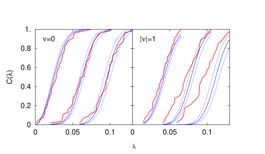
Figure 1: The measured cumulants for the lowest three modes in $\nu=0$ (left) and $|\nu|=1$ (right). The smooth dashed curve represents the RMT prediction with the value of $\Sigma$ from the combined fit to the lowest mode in each sector. The dotted curves indicate the $1\sigma$ range of $\Sigma$ determined by the bootstrap method.

$m$	$a^{3}\Sigma$	$|\nu|$	$N$	CL level 1	CL level 2	CL level 3
0.015	0.0130(7)	0	26	0.82	0.86	0.02
		1	32	0.42	0.15	0.71
0.03	0.0112(7)	0	33	0.12	0.57	0.04
		1	28	0.20	0.13	0.02
0.05	0.0105(4)	0	55	0.55	0.77	0.94
		1	47	0.64	0.01	0.00
0.05	0.0098(5)	0	55	0.52	0.79	0.93
		1	47	0.67	0.02
0.05	0.0111(6)	0	55	0.07	0.03	0.001
		1	47	0.99	0.08	0.0005
0.05	0.0106(4)	0	55	0.52	0.80	0.90
		1	47	0.67	0.02	0.00

Table 1: $a^{3}\Sigma$ from a fit to the lowest eigenvalues on the $10^{4}$ ensembles. The confidence levels for the individual distributions are given in the last three columns; they are boxed if the level is included in the fit.

The result of a combined fit to the lowest mode in each topological sector is shown in Fig. 1. To visualize the range of the uncertainty in $a^{3}\Sigma=0.0105(4)$, we show the theoretical curves for the two extremal values of the one sigma range. The errors on the fit parameter are determined by the bootstrap procedure. (See Fig. 2 (top) for a comparison of the binned data with the RMT distribution.) We find very good agreement for the shape and position of the lowest three modes in $\nu=0$. In $\nu=1$ however, only the lowest mode matches. For all these modes, the confidence levels are above $50\%$. See Table 1 for the confidence levels of the fits to the individual distributions.

Figure 2: RMT fit to eigenvalue distributions for $am_{q}=0.05$, $0.03$ and $0.015$. The value of $a^{3}\Sigma$ is determined from a combined fit to the lowest mode in each topological sector.

To check for consistency between the two topological sectors, we show the results from separate fits of the RMT prediction to the distribution in each topological sector. The general statements from the combined fit persist: The lowest three modes in $\nu=0$ and the lowest one in $|\nu|=1$ can be described by RMT. The extracted values of $a^{3}\Sigma$ agree within uncertainties (the $\nu=0$ ensemble is completely independent from the $|\nu|=1$ ensemble). We get $a^{3}\Sigma=0.0098(5)$ from $\nu=0$ and $a^{3}\Sigma=0.0111(6)$ from $\nu=1$.

So far we have focused on the $am_{q}=0.05$ data set, because of its higher statistics. The streams at $am_{q}=0.03$ and 0.015, however, give us the possibility to check, whether the quark mass dependence of the RMT prediction is correct. From a combined fit to the distribution of the lowest eigenvalue in each topological sector (the fit we also chose to use for our final value for $am_{q}=0.05$), we extract $a^{3}\Sigma=0.0112(7)$ and $a^{3}\Sigma=0.0130(7)$ for $am_{q}=0.03$ and 0.015 respectively. Fig. 2 shows the RMT predictions from these values of $\Sigma$ along with the measured distributions.

The values of $a^{3}\Sigma$ for the three sea quark masses seem to be only barely compatible, however, one has to compare them with the difference in the lattice spacing taken into account. Using the results from Sec. II.3 and Sec. II.4 (to convert our numbers to $\overline{MS}$ regularization scheme) we plot $r_{0}^{3}\Sigma$ as a function of the bare sea quark mass and obtain a reasonable agreement within uncertainties, see Fig. 3. Taking the average of the three values we find $r_{0}^{3}\Sigma=0.368(41)$.

Figure 3: The dimensionless quantity $r_{0}^{3}\Sigma$ in $\overline{MS}$ scheme at $\mu=2$ GeV, as a function of the bare quark mass. The horizontal lines represent the averaged value $r_{0}^{3}\Sigma=0.368(41)$ and its uncertainty.

The measured confidence levels are much better than what we found on smaller lattices which makes us confident that the deviations which we observe are only due to the finite volume. In Ref. DeGrand:2005vb , we simulated on $8^{4}$ lattices with a same lattice spacing. The volume there was clearly too small. To demonstrate the improvement due to the larger volume, we have re-analyzed the data with the techniques described above. The results are given in Table 2 and should be compared to the second and third entry in Table 1, because in both cases we fitted to the lowest mode in each topological sector. We clearly observe an improvement in the confidence level when we go to the larger volume, i.e. the RMT prediction match the measured cumulants much better.

We recall (see Eq. 2) that the result $\Sigma$ of finite simulation volume is equal to $\rho\Sigma_{\infty}$, where $\Sigma_{\infty}$ is the infinite volume condensate. We do not know $\rho$ since we have not measured $f_{\pi}$, but combining our lattice spacing and lattice size with $f_{\pi}=93$ MeV, we expect $\rho\sim 1.42$ for $L=10$ and $\rho(L=10)/\rho(L=8)=0.86$. In order to compare the results from the two volumes, we have to divide each of them by its respective $\rho$. For $m=0.05$ we therefore obtain for the $10^{4}$ lattices $a^{3}\Sigma_{\infty}=0.0074(3)$ and for the $8^{4}$ lattices $a^{3}\Sigma_{\infty}=0.0080(3)$. The error-bars of the two values touch. However, we suspect that the $8^{4}$ data may be too small for RMT to provide a reliable determination of the condensate. We are unwilling to attempt a combined fit of $\rho\Sigma$ in terms of $f_{\pi}$ and $\Sigma$ from data obtained on several simulation volumes without good RMT fits for each volume.

$m$	$a^{3}\Sigma$	$|\nu|$	$N$	CL level 1	CL level 2	CL level 3
0.03	0.0124(5)	0	112	$6\cdot 10^{-5}$	0.06	0.05
		1	58	$9\cdot 10^{-5}$	$0.002$	$1\cdot 10^{-5}$
0.05	0.0132(5)	0	96	0.01	0.004	$0.03$
		1	75	0.04	0.003	0

Table 2: To demonstrate the effect of the finite volume, we also re-analyzed our old $8^{4}$ data. The notation is the same as in Tab. 1. This table corresponds to the second and third entry in Tab. 1 for the $10^{4}$ lattices. The confidence levels are considerably lower.

II.3 Lattice spacing

We determined an overall scale from a fit to the static quark potential. It is extracted from the effective masses of Wilson loops after one level of HYP smearing Hasenfratz:2001hp ; Hasenfratz:2001tw , where the short-distance effects of the HYP smearing are corrected using a fit to the perturbative lattice artifacts. We measured the potential on 76, 82, and 48 $8^{3}\times 12$ configurations at $am_{q}=0.05$, 0.03, and 0.015 (spaced 5 HMC trajectories apart, from several streams per mass). To generate these data sets we used a conventional two-flavor HMC algorithm. Fits with the minimum distance $t=4$ and 5 are consistent within uncertainties. In Ref. DeGrand:2005vb we only had $8^{4}$ lattices, which prevented us from going to these separations. The determinations of $r_{0}/a$ from those data sets are slightly different from what we have here, and were slightly contaminated by excited states. A compilation of fit results is shown in Table 3.

$m_{q}$	$r_{0}/a$	$a$[fm]
0.015	3.47(8)	0.144(3)
0.03	3.27(6)	0.153(3)
0.05	3.35(7)	0.148(3)

Table 3: The Sommer parameter $r_{0}$ and the lattice spacing $a$ in fm from $r_{0}=0.5~{}{\rm fm}$. We show results from two fit ranges used to extract the potential. The fit range for the fit to the potential was $r\in[1.4,6.1]$ with little variation between different choices for this range.

II.4 Conversion to $\overline{MS}$ regularization

A renormalization constant is needed to convert the lattice result of the quark condensate to its $\overline{MS}$ value. To get this matching factor, we use the RI’ scheme introduced in Ref. Martinelli:1994ty . Specifically we follow the procedure described in Ref. DeGrand:2005af . The RI’ scheme result in the chiral limit can be converted to the 2 GeV $\overline{MS}$ value by using the ratio connecting the two schemes. The ratio was computed by continuum perturbation theory to three loops Franco:1998bm ; Chetyrkin:1999pq .

The simulation for getting the matching factor should not be restricted in topological sectors. Also, one needs simulations with a momentum scale short enough to be free from nonperturbative effects and yet not too short to be affected by discretization effects. Somewhat to our surprise, our sample of $8^{4}$ lattices proved suitable to do this. We combined multiple streams of data together to reduce simulation-time autocorrelations. Our data sets consisted of approximately 50 configurations per mass value at two values of the bare sea quark mass, $am_{q}=$0.03 and 0.05.

The $8^{4}$ lattice is periodic in space directions and antiperiodic in the time direction. Therefore the momentum values are

$$ap_{\mu}=\left(\frac{2\pi}{8}k_{x},\frac{2\pi}{8}k_{y},\frac{2\pi}{8}k_{z},\frac{\pi}{8}(2k_{t}+1)\right).$$ (8)

We choose the values of $k_{\mu}$ such that the momentum values lie as close as possible to the diagonal of the Brillouin zone. The maximum value of $ap=2.115$ corresponds to $k_{\mu}=(2,1,0,1)$. The propagators are cast from a point source and then projected to the desired momentum values.

The renormalization constant for the scalar density in the RI’ scheme is given in Fig. 4.

Figure 4: $Z_{S}^{RI^{\prime}}$ for quark mass $am_{q}=0.03$ and 0.05.

Values of $Z_{S}^{RI^{\prime}}$ for $am_{q}=0.03$ and 0.05 are listed in Table 4. The inverse lattice spacings are 1.29 GeV and 1.32 GeV for the $am_{q}=0.03$ and 0.05 data sets determined from the Sommer parameter. Thus $\mu=2$ GeV corresponds to $a\mu=1.55$ or 1.52. The 2 GeV RI’ values are obtained from linear interpolations from the two closest $\mu$ values of the data.

Table 4: Values of $Z_{S}$ in the RI’ scheme for the two quark masses. The inverse lattice spacings are 1.29 GeV and 1.32 GeV for the $am_{q}=0.03$ and 0.05 data sets respectively from the Sommer parameter. Therefore $\mu=2$ GeV corresponds to $a\mu=1.55$ or 1.52 accordingly. The 2 GeV RI’ values are obtained from linear interpolations from the two closest $\mu$ values of the data.

$a\mu$	$am_{q}=0.03$	$am_{q}=0.05$
0.878	0.66(8)	0.77(13)
1.178	0.67(6)	0.82(14)
1.416	0.68(5)	0.70(6)
1.619	0.71(4)	0.75(7)
1.800	0.69(3)	0.77(7)
1.963	0.70(3)	0.70(3)
2.115	0.70(3)	0.71(3)
$\mu=2$GeV	0.70(4)	0.73(6)

The conversion ratio for the scalar and pseudoscalar densities, in Landau gauge and to three loops, is Franco:1998bm ; Chetyrkin:1999pq

$$\frac{Z_{S}^{\overline{\rm MS}}}{Z_{S}^{\rm RI^{\prime}}} = \frac{Z_{P}^{\overline{\rm MS}}}{Z_{P}^{\rm RI^{\prime}}}=1+\frac{16}{3}\frac{\alpha_{s}}{4\pi}+\left(\frac{4291}{18}-\frac{83n_{f}}{9}-\frac{152\zeta_{3}}{3}\right)\left(\frac{\alpha_{s}}{4\pi}\right)^{2}$$ (9)

$$+\left(\frac{3890527}{324}-\frac{241294n_{f}}{243}+\frac{7514n_{f}^{2}}{729}-\frac{224993\zeta_{3}}{54}\right.$$

$$+\left.\frac{4720\zeta_{3}n_{f}}{27}+\frac{32\zeta_{3}n_{f}^{2}}{27}-\frac{80\zeta_{4}n_{f}}{3}+\frac{2960\zeta_{5}}{9}\right)\left(\frac{\alpha_{s}}{4\pi}\right)^{3}+O(\alpha_{s}^{4}),$$

where $n_{f}$ is the number of flavors and $\zeta_{n}$ is the Riemann zeta function evaluated at $n$. This formula is for zero quark mass.

To get numerical results of the above ratio, we use the coupling constant from the so-called “$\alpha_{V}$” scheme. As in the appendix of Ref. DeGrand:2005vb , from the one-loop expression relating the plaquette to the coupling

$$\ln\frac{1}{3}{\rm Tr}U_{p}=-\frac{8\pi}{3}\alpha_{V}(q^{*})W,$$ (10)

where $W=0.366$ and $q^{*}a=3.32$ for the tree-level Lüscher–Weisz action, we obtain $\alpha_{V}(3.32/a)=0.192$ and 0.193 for the $am_{q}=0.03$ and 0.05 data sets. Then $\alpha_{s}^{\overline{MS}}(e^{-5/6}3.32/a)$ is calculated Brodsky:1982gc and run to $\alpha_{s}^{\overline{MS}}$(2 GeV) by using $\beta_{0}=29/12\pi$ and $\beta_{1}=230/48\pi^{2}$ for two flavor QCD. We find $\alpha_{s}^{\overline{MS}}$(2 GeV)$=0.210$ and 0.213 for the $am_{q}=0.03$ and 0.05 data sets respectively. Then from Eq.(9) with $n_{f}=2$, we get $Z_{S}^{\overline{MS}}/Z_{S}^{RI^{\prime}}=1.160$ and 1.164 accordingly. Therefore $Z_{S}^{\overline{MS}}$(2 GeV)$=0.81(5)$ and 0.85(7) for the two data sets. Because these two values have rather large uncertainty, we perform the chiral limit by fitting to a constant and get $Z_{S}^{\overline{MS}}$(2 GeV)=0.83(4).

III Results

Combining our results for the lattice regulated condensate, the Sommer parameter, and the Z-factor, we find $r_{0}^{3}\Sigma(\overline{MS},\mu=2\ {\rm GeV})=0.328(28)$, 0.325(31), and 0.451(45) at $am_{q}=0.05$, 0.03, and 0.015 respectively. These values are plotted in Fig. 3. The result from each quark mass is the parameter of the Chiral Lagrangian. Averaging them, we find

$$r_{0}^{3}\Sigma(\overline{MS},\mu=2\ {\rm GeV})=0.368(41).$$ (11)

Taking the real-world value for $r_{0}=0.5$ fm, this is

$$\Sigma(\overline{MS},\mu=2\ {\rm GeV})=0.0225(25){\rm GeV}^{3}$$ (12)

or

$$(\Sigma(\overline{MS},\mu=2\ {\rm GeV}))^{1/3}=282(10){\rm MeV}.$$ (13)

All of these analyses ignore $\rho$. If we knew $f_{\pi}$, we could divide it out. This would reduce $\Sigma$ by a factor 1/1.42 if $f_{\pi}=93$ MeV. Since we have no lattice determination of $f_{\pi}$ from our simulation, $\rho$ represents a systematic excess, which we must quote separately, 31 MeV for $\Sigma^{1/3}$, for example.

IV Conclusions

A summary of previous calculations of the condensate has recently been given by McNeileMcNeile:2005pd . Comparing the summary of quenched determinations there, a three-flavor prediction by McNeile, our recent $N_{f}=1$ result DeGrand:2006uy of $(\Sigma(\overline{MS},\mu=2\ {\rm GeV}))^{1/3}=0.269(9)$ GeV (which also does not include $\rho$) and our $N_{f}=2$ result quoted above, the condensate seems to be a quantity which is not very $N_{f}$ dependent. Our result is also quite consistent with the Gell-Mann-Oakes-Renner relation, the pion mass and (non-lattice) phenomenological estimates of the up and down quark massesJamin:2002ev .

This project suffers from a too-small simulation volume, relatively low statistics and we just have a single coarse lattice spacing. The small volume is reflected in the limited range of eigenmodes which are well-predicted by RMT and by the factor $\rho$ which is present as a systematic in our final answer. (Recall, $\rho$ approaches unity like $1/L^{2}$). In principle, one could determine $f_{\pi}$ by some other method and scale $\rho$ out of the RMT fit. We also have the usual problem of a lattice simulation at one value of the lattice spacing: scaling violations are unknown. In hindsight, the three masses we did here are overkill; a single small quark mass suffices to give $\Sigma$ from RMT.

In contrast, the strength of this calculation is the use of a chiral lattice fermion, which allows for the preservation of chiral symmetry in the bare action and insures that spontaneous chiral symmetry breaking (and explicit chiral symmetry breaking induced by a quark mass) occurs at finite lattice spacing exactly as in the continuum. From a simulation point of view, critical slowing down turned out to be largely eliminated due to the possibility to run in the opposite chirality sector. The definition of the topological charge by the index of the Dirac operator allows us to easily monitor the topological charge. This makes it possible to produce ensembles at fixed topology which is convenient for the comparison to the predictions of RMT, which are at definite topological charge.

References

- (1) C. McNeile, Phys. Lett. B 619, 124 (2005) [arXiv:hep-lat/0504006].
- (2) H. Neuberger, Phys. Lett. B 417, 141 (1998) [arXiv:hep-lat/9707022].
- (3) H. Neuberger, Phys. Rev. Lett. 81, 4060 (1998) [arXiv:hep-lat/9806025].
- (4) P. H. Ginsparg and K. G. Wilson, Phys. Rev. D 25, 2649 (1982).
- (5) T. DeGrand and S. Schaefer, Phys. Rev. D 72, 054503 (2005) [arXiv:hep-lat/0506021].
- (6) T. DeGrand, R. Hoffmann, S. Schaefer and Z. Liu, Phys. Rev. D 74, 054501 (2006) [arXiv:hep-th/0605147].
- (7) E. V. Shuryak and J. J. M. Verbaarschot, Nucl. Phys. A 560, 306 (1993) [arXiv:hep-th/9212088].
- (8) J. J. M. Verbaarschot and I. Zahed, Phys. Rev. Lett. 70, 3852 (1993) [arXiv:hep-th/9303012].
- (9) J. J. M. Verbaarschot, Phys. Rev. Lett. 72, 2531 (1994) [arXiv:hep-th/9401059].
- (10) M. E. Berbenni-Bitsch, S. Meyer, A. Schäfer, J. J. M. Verbaarschot and T. Wettig, Phys. Rev. Lett. 80, 1146 (1998) [arXiv:hep-lat/9704018].
- (11) P. H. Damgaard, U. M. Heller and A. Krasnitz, Phys. Lett. B 445, 366 (1999) [arXiv:hep-lat/9810060].
- (12) M. Göckeler, H. Hehl, P. E. L. Rakow, A. Schäfer and T. Wettig, Phys. Rev. D 59, 094503 (1999) [arXiv:hep-lat/9811018].
- (13) R. G. Edwards, U. M. Heller, J. E. Kiskis and R. Narayanan, Phys. Rev. Lett. 82, 4188 (1999) [arXiv:hep-th/9902117].
- (14) L. Giusti, M. Lüscher, P. Weisz and H. Wittig, JHEP 0311, 023 (2003) [arXiv:hep-lat/0309189].
- (15) E. Follana, A. Hart, C. T. H. Davies and Q. Mason [HPQCD Collaboration], Phys. Rev. D 72, 054501 (2005) [arXiv:hep-lat/0507011].
- (16) J. Wennekers and H. Wittig, JHEP 0509, 059 (2005) [arXiv:hep-lat/0507026].
- (17) M. E. Berbenni-Bitsch, S. Meyer and T. Wettig, Phys. Rev. D 58, 071502 (1998) [arXiv:hep-lat/9804030].
- (18) P. H. Damgaard, U. M. Heller, R. Niclasen and K. Rummukainen, Phys. Lett. B 495, 263 (2000) [arXiv:hep-lat/0007041].
- (19) P. H. Damgaard and S. M. Nishigaki, Phys. Rev. D 63, 045012 (2001) [arXiv:hep-th/0006111].
- (20) W. Bietenholz, K. Jansen and S. Shcheredin, JHEP 0307, 033 (2003) [arXiv:hep-lat/0306022].
- (21) J. Gasser and H. Leutwyler, Phys. Lett. B 184, 83 (1987); Nucl. Phys. B 307, 763 (1988). See also P. Hasenfratz and H. Leutwyler, Nucl. Phys. B 343, 241 (1990).
- (22) A. Bode, U. M. Heller, R. G. Edwards and R. Narayanan, arXiv:hep-lat/9912043.
- (23) N. Cundy, Nucl. Phys. Proc. Suppl. 153, 54 (2006) [arXiv:hep-lat/0511047].
- (24) T. DeGrand and S. Schaefer, JHEP 0607, 020 (2006) [arXiv:hep-lat/0604015].
- (25) R. Sommer, Nucl. Phys. B 411, 839 (1994) [arXiv:hep-lat/9310022].
- (26) G. Martinelli, C. Pittori, C. T. Sachrajda, M. Testa and A. Vladikas, Nucl. Phys. B 445, 81 (1995) [arXiv:hep-lat/9411010].
- (27) S. Duane, A. D. Kennedy, B. J. Pendleton and D. Roweth, Phys. Lett. B 195, 216 (1987).
- (28) Z. Fodor, S. D. Katz and K. K. Szabo, JHEP 0408, 003 (2004) [arXiv:hep-lat/0311010].
- (29) T. DeGrand and S. Schaefer, Phys. Rev. D 71, 034507 (2005) [arXiv:hep-lat/0412005].
- (30) S. Schaefer and T. A. DeGrand, PoS LAT2005, 140 (2005) [arXiv:hep-lat/0508025].
- (31) M. Lüscher and P. Weisz, Commun. Math. Phys. 97, 59 (1985) [Erratum-ibid. 98, 433 (1985)].
- (32) M. G. Alford, W. Dimm, G. P. Lepage, G. Hockney and P. B. Mackenzie, Phys. Lett. B 361, 87 (1995) [arXiv:hep-lat/9507010].
- (33) C. Morningstar and M. J. Peardon, Phys. Rev. D 69, 054501 (2004) [arXiv:hep-lat/0311018].
- (34) M. Hasenbusch, Phys. Lett. B 519, 177 (2001) [arXiv:hep-lat/0107019].
- (35) Numerical Recipes in C: The art of scientific computing, 2nd ed, W.H. Press, S.A. Teukolsky, W.T. Vetterling and B.P. Flannery, Cambridge Univ. Pr., 1995.
- (36) T. DeGrand and Z. F. Liu, Phys. Rev. D 72, 054508 (2005) [arXiv:hep-lat/0507017].
- (37) E. Franco and V. Lubicz, Nucl. Phys. B 531, 641 (1998) [arXiv:hep-ph/9803491].
- (38) K. G. Chetyrkin and A. Retey, Nucl. Phys. B 583, 3 (2000) [arXiv:hep-ph/9910332].
- (39) A. Hasenfratz and F. Knechtli, Phys. Rev. D 64, 034504 (2001) [arXiv:hep-lat/0103029].
- (40) A. Hasenfratz, R. Hoffmann and F. Knechtli, Nucl. Phys. Proc. Suppl. 106, 418 (2002) [arXiv:hep-lat/0110168].
- (41) S. J. Brodsky, G. P. Lepage and P. B. Mackenzie, Phys. Rev. D 28, 228 (1983).
- (42) M. Jamin, Phys. Lett. B 538, 71 (2002) [arXiv:hep-ph/0201174].