Precision lattice QCD calculations and predictions of fundamental physics in heavy quark systems

Abstract

I describe the recent success in performing accurate calculations of the effects of the strong force on particles containing bottom and charm quarks. Since quarks are never seen in isolation, and so cannot be studied directly, numerical simulations are key to understanding the properties of these particles and extracting information about the quarks. The results have direct impact on the worldwide experimental programme that is aiming to determine the parameters of the Standard Model of particle physics precisely and thereby uncover or constrain the possibilities for physics beyond the Standard Model. The numerical simulation of the strong force is a huge computational task and the recent success is the result of international collaboration in developing techniques that are fast enough to do the calculations on powerful supercomputers.

1 Introduction - the physics problem

The aim of particle physics is to uncover the fundamental particles and interactions that drive physics at the smallest distance scales.

This is often represented as ‘peeling away the layers of an onion’ starting with the atom as the outside layer. In fact it is rather more complicated. The subunits of the atomic nucleus have been known for seventy-five years. They are called protons and neutrons and are very similar particles although the proton has electrical charge equal to, but opposite in sign, to that of the electron and the neutron is electrically neutral. Protons and neutrons can be relatively easily isolated and studied in the laboratory and their mass and charge determined. Indeed protons accelerated to very high energies are one of the key experimental tools in studying particle physics at laboratories such as Fermilab and CERN. When high energy protons collide, a huge myriad of other particles is produced that can be tracked in particle detectors and their electrical charge and mass measured. These particles are not, however, the subunits of the proton. In fact, apart from the electron and its partners the muon and tau, they are particles made themselves of the same subunits as the proton. These subunits are known as quarks and particles made of them are collectively called hadrons. We have never been able to isolate quarks and so can only infer their existence from the results of these experiments using theoretical understanding. The existence of quarks is now universally accepted, but the problem that they are never seen as free particles makes it even harder to ‘peel away another layer of the onion’. A key requirement for progress on this will be precise determination of the properties of quarks and, because of the nature of quarks, this requires both precise experimental results and precise theoretical calculations. Lattice QCD aims to provide these theoretical calculations.

1.1 The Standard Model

The Standard Model of particle physics describes the particles and interactions at the most fundamental level currently known. There are three forces described by the Standard Model. The simplest and the one that we have most every day experience of is electromagnetism. At the every day level we can use the classical theory of Maxwell’s equations that deals with electric and magnetic fields and the interaction of electrically charged particles with those fields. When we are dealing with the small distances of the subatomic world we must convert this to a quantum theory that can handle phenomena such as the production of particles and antiparticles out of the energy of an electromagnetic field. In the quantum theory electrically charged particles, such as the electron, are described by a quantum field, $\psi(x)$. The particles interact by exchange of the quanta of the electromagnetic field, called photons, with quantum field $A_{\mu}(x)$. The Lagrangian of the theory is particularly elegant, possessing a symmetry called a local gauge symmetry, that so limits the types of interactions that are allowed, and constrains the theory to be well-behaved, that it can be taken as a requirement rather than a result. The fact that the other two forces described by the Standard Model, the weak force and the strong force, are also gauge theories with a local gauge symmetry is then very satisfying. It took some time to realise that this was true, however, because at first sight the weak and strong forces look very different from electromagnetism.

The strong force operates inside the atomic nucleus between the protons and neutrons and keeps the nucleus together against the electrical repulsion of the protons. The electrical force operates over relatively large distance scales - it keeps the electrons attracted to the atomic nucleus in an atom after all. Playing with fridge magnets is a simple demonstration of this fact in the every day world. The long range is associated with the fact that the photon is a massless particle, a consequence of the gauge symmetry of the theory. Instead the strong force is limited to the short range of the atomic nucleus and therefore seems to require a massive exchange particle. The interaction between protons and neutrons is not fundamental, however, but is the ‘left-over’ result of the interaction between the quarks inside the protons and neutrons.

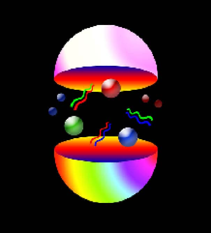
Figure 1: The proton is made of 3 valence quarks (shown as large spheres) - 2 $u$ quarks and a $d$ quark in a complicated and strongly interacting soup of gluons and sea quark-antiquark pairs (of flavors $u$, $d$ and $s$ and shown as small spheres). The whole object has no color charge and so can exist as a free particle, unlike the quarks or gluons themselves. There are six quark flavors, arranged into three ‘generations’, given below as 2-d vectors. Each generation has a quark of electrical charge $-e/3$ (the top entry in the vector) and a quark of charge $+2e/3$ (the lower entry). $\quad\quad\quad\quad\quad\displaystyle{d\choose u}{s\choose c}{b\choose t}$

1.2 QCD as the theory of the strong force

It turns out that the strong force can be described by a gauge theory called quantum chromodynamics (QCD) and this theory is very similar to quantum electrodynamics (QED) except that the equivalent of electrical charge, called color charge, comes in three possibilities instead of just being a number. The gauge symmetry of QCD is then described by a different gauge group and this gives rise to the very different behaviour of the strong force. Quarks carry an electrical charge which is either -2/3 or +1/3 times the charge on a electron, $-e$, (the basic unit of electrical charge). Their color charge however is a vector of length the basic unit of color charge, $g$, but in a three-dimensional space with axes called red, green and blue. The antimatter partners of the quarks, antiquarks, have opposite electrical charge (just as the antielectron, or positron, has charge $+e$) and color charge anti-red, anti-blue or anti-green. The exchange particle, called the gluon, is massless like the photon but also carries a color charge, whereas the photon has no electrical charge. The gluon in fact has both a color and an anti-color charge in eight combinations. This means that gluons, as well as quarks, can emit gluons. It is this possibility that is at the root of the counter-intuitive behaviour of the strong force.

We are used to thinking of electrical charge as being a measurable and fixed quantity - some number of units of $e$. It is determined in principle by taking a test charge at some distance from the charge in question and measuring the strength of the interaction between them. In fact, at the small distances of the subatomic world, the charge measured in this way depends on the distance at which it is measured. Electrical charge appears to get stronger as you get closer to it. This is a result, in QED, of ‘vacuum polarisation’ by which photons, produced by energy fluctuations in the vacuum, decay into an electron-positron pair that screen the charge in the same way that charge is screened inside a dielectric medium. As you get closer to the charge the screening is less effective and the charge seen increases. For color charge the opposite result occurs - gluons in the vacuum can produce screening quark-antiquark pairs but also ‘antiscreening’ gluons. The antiscreening wins out over the screening so that color charge gets smaller as you get closer to it and the strong interaction between color charges gets weaker. This is known as ‘asymptotic freedom’ and Gross, Politzer and Wilczek showed that QCD demonstrated this property in 1973 (and shared the 2004 Nobel Prize).

QCD seems to have the right properties to explain the basic features of the strong force. Experiments in which electrons are fired with high energy at protons (therefore probing short distances inside the proton) show that the constituents of the proton are basically behaving like free particles with rather weak strong force interactions. When high energy protons collide together the hadrons that spray out from the interaction do so in a way that bears the imprint of a basic strong force interaction in which a quark-antiquark pair were produced and flew apart, perhaps weakly emitting gluons. We cannot see this basic interaction directly because as the quark and antiquark separate more quarks, antiquarks and gluons are produced from the interaction energy so that only hadrons, bound states of quarks, antiquarks and gluons that have no overall color charge, can be seen in particle detectors (see Figure 1). Theoretical calculations in QCD can be done analytically for these high energy, short distance, examples where the strong force is relatively weak. Then the so-called ‘coupling constant’, $\alpha_{s}=g^{2}/4\pi$, is relatively small and a powers series expansion in the number of interactions, or powers of $\alpha_{s}$, makes sense. This is the standard approach, known as perturbation theory, for QED where $\alpha_{em}=e^{2}/4\pi$ is naturally very small and it allows us to test QED to fantastic precision. Good tests of QCD are also possible for specific results from high energy collisions that survive the conversion from quarks into hadrons.

QCD can tell us more than this, however. In principle all the properties of hadrons are predictable from QCD once the free parameters of the theory, the quark masses and $g$, are fixed. In practice this is a very difficult problem since at the typical distance scales inside a hadron, the strong interaction is very strong and $\alpha_{s}$ very large. Perturbation theory is no guide since it is no longer true that including more interactions in the calculation (and therefore higher powers of $\alpha_{s}$) gives a smaller number. Instead any number of interactions is equally important and the theory becomes non-linear and very complicated. It has after all to generate the phenomenon by which quarks are confined within hadrons and cannot escape to be free particles. Numerical simulation is the only way to solve this and, as we shall see in the next section, is an enormous computational task.

An issue that complicated the understanding of results from high energy experiments was the sheer number of different hadrons that there are, each one with a distinct mass and having various electrical charges and spins. Some hadrons live for long enough to be seen distinctly in particle detectors (such as protons); others live for only a short time, and their existence must be reconstructed from the tracks of longer lived decay products. We now know that the reason for this ‘particle zoo’ is that there are six different types or ‘flavors’ of quarks. They are dubbed ‘up’, ‘down’, ‘strange’, ‘charm’, ‘bottom’ and ‘top’ quarks, in order of increasing mass, and abbreviated by their initials: $u$, $d$, $s$, $c$, $b$, and $t$. The $d$, $s$ and $b$ quarks have electrical charge $-e/3$ and the $u$, $c$ and $t$ quarks have electrical charge $2e/3$. In fact the heaviest quark, the top quark, does not live for long enough to make interesting bound states, so the hadrons that we can study have as basic constituents different combinations of the five lighter quarks. This gives a very rich physics because the quarks can be put together in many combinations and within those combinations different spin orientations and different amounts of orbital angular momentum give different hadrons. All of the hadrons should be described by QCD, however, and as we shall see it can be simpler to do QCD calculations for some of the more esoteric short-lived hadrons than for the long-lived every day proton. Here I will describe mainly results for particles made of charm and bottom quarks.

1.3 The weak force

As well as the electromagnetic and strong forces quarks are also subject to the third force of the Standard Model, the weak force. This force is best known for its effects in nuclear beta decay. In that process the atomic nucleus of one element changes to that of another and emits a beta ray (an electron). In fact what is happening is that a down quark in a neutron in the original nucleus changes to an up quark and emits a $W-$ boson. Since a neutron has as basic constituents two $d$ quarks and a $u$, $ddu$, and the proton is $uud$ then the neutron changes to a proton in this process. The original nucleus thus changes to that of the element with one higher atomic number. The $W$ boson is the exchange boson of the weak force and that decays to an electron, which is detected, and an anti-neutrino, which is very hard to see. The weak force was also originally hard to fit into the pattern of a gauge theory set by QED because the $W$ boson has a mass. However, again this was misleading and the result of spontaneous breaking of the weak force gauge symmetry caused by the Higgs boson.

Weak force interactions are the only way for a quark to change flavor. Since the $W$ boson is electrically charged with charge $+e$ for $W^{+}$ and $-e$ for $W^{-}$, when a quark emits a $W$ boson it changes flavor from one of the three $+2e/3$ quarks to one of the $-e/3$ set or vice versa. The existence of the Higgs boson and the quark interactions with that boson mean that the coupling between the different quark flavors and the W boson are not all the same but appear as a $3\times 3$ matrix (the Cabibbo-Kobayashi-Maskawa or CKM matrix) that can have complex numbers for coefficients. This has the interesting consequence that the symmetry between matter and antimatter can then be broken. We know that this symmetry is broken in the real world since we live in a universe made of matter which presumably started from a symmetric equal mixture of matter and antimatter at the Big Bang. However what we don’t know is whether the description of this breaking through the $3\times 3$ CKM matrix is the correct one. The first stage in this process is to determine the elements of this matrix accurately and in particular to discover whether it is a unitary matrix as required by the Standard Model picture. The matrix connects the $+2e/3$ quarks to the $-e/3$ charged quarks with entries:

$$\left(\begin{array}[]{ccc}{\bf V_{ud}}&{\bf V_{us}}&{\bf V_{ub}}\\ {\bf V_{cd}}&{\bf V_{cs}}&{\bf V_{cb}}\\ {\bf V_{td}}&{\bf V_{ts}}&{\bf V_{tb}}\\ \end{array}\right)$$

If this matrix turned out not to be unitary, it would be the ‘smoking gun’ of physics beyond the Standard Model.

A large part of the current particle physics experimental programme is devoted to this effort. It turns out that critical elements of this matrix can be obtained by the study of the weak interactions of the $b$ quark. The $b$ quark will emit a $W^{-}$ boson that can decay to an electron and antineutrino by analogy to the $d$ quark interaction that is nuclear $\beta$ decay described above. At a simple level the rates of the weak decay of the $b$ quark to the different $2e/3$ quarks are proportional to the squares of the appropriate elements of the CKM matrix. However, as described earlier, $b$ quarks cannot be found in isolation but only bound into hadrons. The QCD interactions inside the hadron affect the decay rate and must be calculated precisely in order to extract the appropriate CKM matrix element from the experimental result. This must be done in lattice QCD and, as we shall see, is one place where lattice QCD is now making a big contribution and will provide key results in the near future.

2 Introduction - the computational problem

A quantum field theory can be defined by its Feynman path integral and this is a convenient way to express it for numerical simulation. This formulation has a lot of overlap with statistical mechanics and shares some common language. The basic integral is often called the partition function and for a gauge theory is expressed as:

$$Z=\int dA_{x\mu}d\psi_{x}d\overline{\psi}_{x}exp(iS(A,\psi,\overline{\psi}))$$ (1)

where the integral is over the field variables of the gluon ($A_{\mu}$) and quark fields ($\psi,\overline{\psi}$) at every point in 4-d space-time, $x$. $S$ is the action of the theory, the space-time integral over the Lagrangian and a function of the gluon and quark fields. The advantage of expressing the theory in this way is that the left-hand side is a quantum transition amplitude, in fact from the vacuum state to the vacuum state, but the right-hand side expresses this as an integral over classical field variables that can be represented as numbers on a computer. The integral sums over all paths (configurations of the $A$ and $\psi$ fields) between the initial and final quantum states weighting each path with $e^{iS}$. In the continuous space-time of the real world this integral is not well-defined because it has infinitely many dimensions if there are infinitely many space-time points and the field variables are unconstrained.

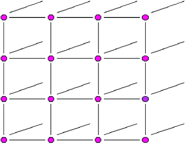
Figure 2: A 2-dimensional rendition of a 3-dimensional lattice. Lattice QCD uses 4-dimensional lattices, usually periodically joined into a 4-dimensional torus. The spacing between the points (and therefore the smallest non-zero distance on the lattice) is denoted $a$. The largest momentum that can be represented meaningfully on the lattice is $\pi/a$ so the lattice provides an ultraviolet cut-off on momenta.

To adapt the integral for numerical solution several steps are needed:

• take a finite box of space-time, of length $L$ on a side

• split the box up into a finite number of points in a 4-dimensional lattice grid. Call the spacing of the grid the lattice spacing, $a$, see Figure 2. The gluon field variables live on the links of the lattice and the quarks on the sites.

• Discretise the interactions of the QCD Lagrangian onto the space-time lattice. The integral is now finite.

• rotate time to imaginary time so that the oscillatory factor $e^{iS}$ becomes the exponential factor $e^{-S}$. Now paths with large action are exponentially suppressed and we can compute the integral using the methods of importance sampling.

The simplest quantum transition amplitudes that we are interested in calculating involve making hadrons out of the vacuum, propagating those hadrons for a certain length of lattice time that allows their energy to be determined, and then destroying them back into the vacuum. This amplitude is then given by

$$\langle 0|H(T)H^{{\dagger}}(0)|0\rangle=\frac{1}{Z}\int dA_{x\mu}d\psi_{x}d\overline{\psi}_{x}H(\psi,\overline{\psi})_{T}H^{{\dagger}}(\psi,\overline{\psi})_{0}\exp(-S(A,\psi,\overline{\psi})).$$ (2)

A further important adaption must now be made because of the nature of quarks. They are fermions (particles with half-integer spin) and therefore obey fermion statistics. This means that their field variables must be anticommuting numbers that cannot be represented on a computer (at least not without enormous difficulty). Instead we must integrate over the $\psi$ and $\overline{\psi}$ fields by hand and this can be done because of the simple way that these fields appear in the Lagrangian. They appear in the form $\overline{\psi}M\psi$ where $\psi$ is a vector representing the quark field on every site of the lattice and $M$ is an (enormous) matrix linking every site on the lattice to every other site, and a function of the gluon fields. Then the quantum transition amplitude above becomes (for a particularly simple hadron $H$ which is a meson made of a quark and an antiquark):

$$\langle 0|H(T)H^{{\dagger}}(0)|0\rangle=\frac{1}{Z}\int dA_{x\mu}{\rm Tr}(M^{-1}_{0T}M^{-1*}_{0T})\det{M}\exp(-S_{g}(A)).$$ (3)

The integral is now over the gluon fields only. $S_{g}$ is that part of the QCD Lagrangian that depends only on the gluon fields and $M$, as explained above is the quark interaction matrix that is also a function of the gluon fields. $M^{-1}$ is its inverse, $\det{M}$ its determinant and Tr is a trace over various matrix indices.

How we proceed to calculate this ratio of path integrals is by first generating sets of ‘configurations’ of gluon fields with a probability related to how much they will contribute to this integral. We can think of them as ‘typical snaphots of the QCD vacuum’. A gluon field configuration is a complete set of values for the gluon field on every link of lattice. The probability distribution for the configurations is $\det{M}\exp(-S_{g})$. Starting with a random configuration, and using algorithms such as the hybrid Monte Carlo algorithm, we generate a long Markov chain of configurations which converges to this probability distribution. We can then record a configuration every so often to make an ensemble of configurations with the right distribution. ‘Every so often’ means a spacing in Markov chain time that allows the configurations to be reasonably independent of each other. Typically there would be five hundred or so configurations in the ensemble.

We then move to the ‘data analysis’ stage of the calculation. Many people can calculate different quantities of the form given in equation 3 from the same ensembles of gluon field configurations so the process divides naturally into two rather like, for example, a particle physics experiment in which the generation of the data and its analysis are separate but linked activities. At the data analysis stage, the integral in equation 3 is evaluated by simply ‘measuring’ (ie. calculating) the value of ${\rm Tr}M^{-1}_{0T}M^{-1*}_{0T}$ on every gluon field configuration and averaging over the ensemble. The factors of $1/Z\det{M}e^{-S_{g}}$ are taken care of by the probability distribution of the configurations in the ensemble, provided we have a good statistical sample. There will be statistical errors associated with the number of independent configurations we have generated. Systematic errors in the result will be discussed below.

An integral like equation 3 has an expected form as a function of $T$ that we can then fit to extract quantities like the mass of hadron $H$, and amplitudes for simple decay processes (see the next section for what kind of decay processes these are). It is important to realise that the raw results are all in units of the lattice spacing, ‘lattice units’. The lattice spacing does not appear explicitly anywhere in the calculation but is implicitly controlled by the parameter $g$ in the QCD Lagrangian. We first have to determine what it is from the results of one calculation before we can convert the results for other calculations from lattice units to physical units. Physical units for masses would be kg but as particle physicists it is natural to use energy equivalents in electron-volts, where the energy equivalent of the mass of a proton is then roughly 1 ${\rm GeV}$. From fitting a hadron correlator (the result for equation 3) we obtain a hadron mass in the form $m_{H}a$ in lattice units. Given a number for $m_{H}a$ and an energy value for $m_{H}$ from experiment in ${\rm GeV}$ we can obtain $a^{-1}$ in ${\rm GeV}$. Then, using this value of $a^{-1}$ results for other hadron masses obtained from the correlators in the form of equation 3 for other hadrons can be converted from lattice units to physical units and compared with experiment.

2.1 Discretisation errors

The use of a lattice and a lattice spacing is simply a device to make the calculation tractable and results in physical units should not depend on the lattice spacing to be reliable. Of course the results do depend on $a$ because of discretisation errors. These errors arise when the QCD Lagrangian is discretised on to the lattice in the same way that they do when all differential equations from continuous space-time are discretised onto a lattice for numerical solution. For example, a derivative can be discretised as a simple finite difference. This is correct as $a\rightarrow 0$ but at finite values of $a$ we can expand the difference in terms of continuum derivatives to see that there are errors at $\cal{O}$$(a^{2})$.

$$\frac{\partial\psi(x_{j})}{\partial x}=\frac{\psi(x_{j}+a)-\psi(x_{j}-a)}{2a}+{\cal{O}}(a^{2})$$ (4)

Most calculations are done at values of $a$ around 0.1fm which corresponds to $a^{-1}$ of 2 GeV. A typical scale for discretisation errors might be 0.5 GeV in which case an $a^{2}$ error might be expected to be $(0.5/2)^{2}$ = 6%. This error is rather too large to accept for a precision calculation, even allowing for the possibility of obtaining results at several values of $a$, fitting the $a$ dependence and so removing it with some error. One problem is that going to smaller values of $a$ rapidly becomes extremely expensive as the cost of the calculation grows as something like $a^{-7}$. A lot of work was done during the 1990s to study discretisation errors in lattice QCD and reduce them further.

In a quantum field theory like QCD further improvement of discretisation errors is not completely straightforward. The usual solution would be to remove the $a^{2}$ error by adding terms from a higher order differencing scheme to cancel it. This removes the leading $a^{2}$ error in lattice QCD but there are sizeable subleading errors. The point of an improved discretisation scheme is to make the equations more closely resemble those in continuous space-time. For QCD, however, the quark fields are radiating gluon fields at all length scales. The difference then between the lattice discretisation and the continuum equations is affected by the fact that in continuous space-time very short-distance interactions can occur, with length scale smaller than the lattice spacing, that are not allowed in lattice QCD. Luckily we know that in this regime the QCD coupling constant becomes rather weak and so we can calculate this difference, and adjust for it, as a power series expansion in $\alpha_{s}$. This has allowed a very successful programme of the improvement of discretisation errors in lattice QCD. The results you will see in the results section have applied this programme to reduce discretisation errors to the few percent level, and to quantify the remaining errors by looking at results at more than one value of $a$.

2.2 Valence quarks and sea quarks

The reason that lattice QCD calculations are so computationally demanding is the presence of the factors of $M^{-1}$ and $\det{M}$ in equation 3. These factors come from the quark fields in QCD but have effectively two somewhat different sources. We say that the $M^{-1}$ factors come from the ‘valence quarks’ and the $\det{M}$ factors come from the ‘sea quarks’. The picture in Figure 1 should make this distinction clear. The basic constituents of a hadron are 3 quarks if it is a baryon and a quark and an antiquark if it is a meson. We have already discussed the neutron as being made of $ddu$ and the proton as being $uud$ (both are baryons). These quarks are known as the valence quarks and they dominate the properties and behaviour, for example in terms of decay modes, of the hadron. However, these quarks are living in a strongly interacting environment inside the hadron. This environment will contain lots of gluon radiation and quark-antiquark pairs made from this gluon radiation. These quark-antiquark pairs are known as the sea quarks. We have already discussed how these quark-antiquark pairs screen color charge and how that is offset by gluon radiation that has an antiscreening effect. If the sea quarks were missing, it is clear that there would be too much antiscreening and we could expect that the coupling constant $\alpha_{s}$ would not vary in the correct way with distance and this would introduce errors.

The inclusion of the $\det{M}$ factor is enormously costly in terms of computer time. Early lattice calculations missed it out in an approximation known as the ‘quenched approximation’. This was indeed wrong, as described above, but it took some while to pin this down because of the lack of understanding of discretisation errors in the early days. Now it is clear that the errors from using the quenched approximation are of order 20% (see Figure 3 in the section on results).

The new lattice calculations include sea quarks and are a huge improvement in terms of accuracy. The important sea quarks are those of lightest mass, $u$, $d$ and $s$, since they can most easily be made from energy fluctuations in the vacuum. Unfortunately the cost of including $\det{M}$ grows as the quark mass gets smaller so for the particularly light $u$ and $d$ quarks we have to operate in the calculation with masses above their physical values and extrapolate down to the real world result, guided by theoretical expectations. If we are close enough to the physical point, this extrapolation does not introduce significant error.

The computing cost for including $\det{M}$ is very large. The improved staggered formulation is the most efficient formulation we have for doing this and also the one with the most mature results (to be described in the next section). For that formulation ongoing calculations to generate an ensemble of gluon field configurations including sea $u$, $d$ and $s$ quarks on a $48^{3}\times 144$ lattice with spacing $a=0.06$fm will take 0.5 - 1.5 Tflopyears depending on the $u/d$ quark mass.

3 Results from lattice QCD

The MILC collaboration has made ensembles of gluon configurations including 2+1 flavours of sea quarks. The ‘2’ refers to sea $u$ and $d$ quarks which are taken to have the same mass for simplicity; the ‘1’ refers to the sea $s$ quark. The formalism used for the quarks is the improved staggered one [1], also known as asqtad. The sea $u/d$ quarks have various masses (for different ensembles) down to $m_{s}/10$ which is about a factor of two from the real world, and much lower than previous calculations. It is then possible to extrapolate to the real world value of the $u/d$ quark mass guided by chiral perturbation theory which dictates the behaviour of quantities as the $u/d$ quark mass goes to zero, and should be valid for sufficiently small $u/d$ mass. There is no numerical problem in reaching the correct $s$ quark mass but, since it is only possible after the calculation to work what the $s$ quark mass was, ensembles with different values of the $s$ quark mass are needed for interpolation purposes.

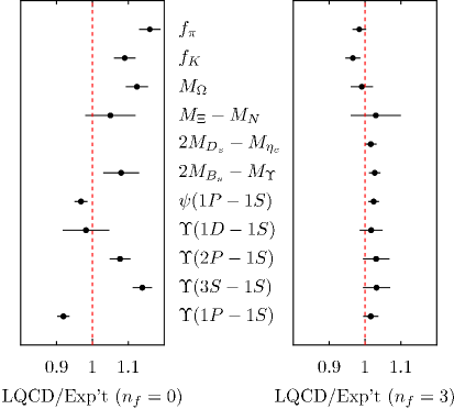
Figure 3: Lattice QCD divided by experiment for eleven different quantities for a range of hadrons. From the top: the decay constants of the $\pi$ ($u\overline{d}$) and $K$ ($u\overline{s}$) mesons; the $\Omega$ ($sss$) baryon mass; a mass difference between the $ssu$ baryon and the proton ($N$) which is insensitive to the $u/d$ mass; the difference between twice the $D_{s}$ ($c\overline{s}$) meson mass and the $\psi$ mass; the difference between twice the $B_{s}$ ($b\overline{s}$) meson mass and the $\Upsilon$ ($b\overline{b}$) mass; the orbital excitation energy in the $\psi$ ($c\overline{c}$) system; various excitations energies in the $\Upsilon$ system. On the left, results in the quenched approximation. On the right, results on the MILC configurations including sea quarks.

There are three sets of ensembles with three different values of the lattice spacing: the ‘fine’ set with $a\approx$ 0.09 fm; the ‘coarse’ set with $a\approx$ 0.12fm and the ‘supercoarse’ set with $a\approx$ 0.18fm. This enables a test of the remaining discretisation errors. At each value of the lattice spacing, as $m_{u/d}$ is changed, the other parameters in the action are adjusted to keep $a$ roughly the same. This is important to avoid confusing effects, including discretisation errors, from changing $a$ with effects from changing $m_{u/d}$. The super-coarse configurations have $16^{3}\times 48$ lattice points, the coarse $20^{3}\times 64$ and the fine $28^{3}\times 96$ in general. The physical volume in all cases then is around $(2.5{\rm fm})^{3}$ in the spatial directions which should be large enough to avoid significant errors from not having a big enough box of space-time. Larger physical volumes have been used for the lightest $u/d$ masses where these effects become more important.

The analysis on these configurations has been done by the Fermilab, HPQCD, MILC and UKQCD collaborations. Most of the results come from the ‘fine’ and ‘coarse’ ensembles. QCD has five parameters for this situation: four quark masses and a coupling constant. These parameters can be fixed by direct comparison of five hadron masses to experiment. The hadron masses used should be sensitive to the parameter being fixed but preferably not to any of the others. First the lattice spacing is fixed from the difference in mass between two mesons with the valence configuration $b\overline{b}$. These mesons are the ‘ground-state’ of this system, called the $\Upsilon$ and its first radial excitation, the $\Upsilon^{\prime}$. This mass difference is useful because it is in fact very insensitive to (all) quark masses. Then the $u/d$ quark mass is fixed from $M_{\pi}$, the $s$ quark mass from $M_{K}$, the $c$ quark mass from $M_{D_{s}}$ and the $b$ quark mass from $M_{\Upsilon}$. Further hadron masses and simple properties like decay constants can then be calculated as a precision test both of lattice QCD and of QCD itself in this strongly coupled regime. The results are shown for eleven different quantities covering the enormous range of QCD physics in Figure 3 (an updated version of that in reference [2]). Note that there are no free parameters in this plot since they have been fixed, as described above, by five quantities that are not shown.

Each plotted point in Figure 3 is the ratio of the lattice QCD result to experiment, and the line marks the correct result i.e. 1. On the left are results using the quenched approximation in which sea quarks are ignored. It is clear then that a number of the results have significant (10-20%) errors. On the right are results from the MILC configurations. Now the results agree with experiment across the board with small errors. This also means that the QCD parameters are unambiguous, as they must be for real QCD - any of the quantities on the plot could have been used instead to determine the parameters and the same result would have been obtained.

3.1 Determining the parameters of QCD

Lattice calculations provide a very direct and accurate way to determine the parameters of QCD: the coupling constant and the quark masses. These parameters come from some ‘theory of everything’ and so can only be determined currently from comparison of QCD to experiment. This means giving up a number of predictions for hadron masses, as described above, equal to the number of parameters. The power of QCD is the huge range of physics addressed with so few parameters, and knowing the parameters accurately can constrain theories of their origin.

The value of the QCD coupling constant, $\alpha_{s}$, could be obtained simply from the determination of the lattice spacing $a$ and knowing the value of $g$ in the action. In fact it can be done more accurately by ‘measuring’ little loops of gluon fields on the lattice (typically one or two lattice spacings wide) given a calculation of these loops as a power series in $\alpha_{s}$. This perturbative series is valid for these short-distance quantities for the small lattice spacing values of the fine and coarse MILC lattices but we do need a series out to third order in $\alpha_{s}$ which is a very hard calculation. The result is shown in Figure 5, with $\alpha_{s}$ converted to a value at a reference distance scale and compared to results using other methods of combining theory and experiment. The lattice QCD result is the most accurate to date [3].

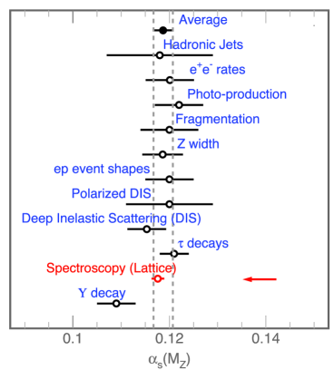
Figure 4: The determination of the QCD coupling constant, $\alpha_{s}$, at a reference scale $M_{Z}$ from a number of methods. The lattice QCD result of 0.1170(12) is the most accurate.

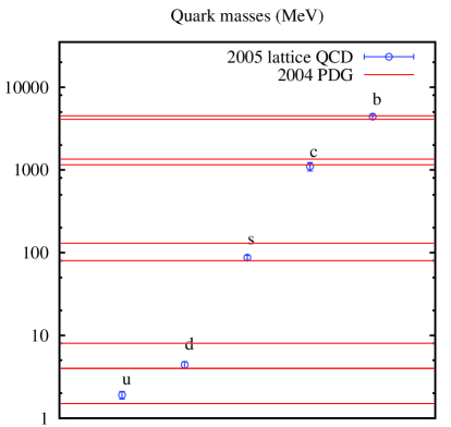
Figure 5: Quark masses from lattice QCD compared to results obtained from other methods quoted in the 2004 Particle Data Tables (red lines). For reference the proton mass is 1000 MeV.

The determination of quark masses from lattice QCD calculations is even more straightforward. Indeed lattice QCD calculations provide a very clear definition of the quark mass, which is otherwise rather hard to pin down when confinement does not allow free quarks to appear. We simply have to adjust the quark mass parameter in the lattice QCD action until the mass of a hadron, preferably one that depends strongly on the quark mass, agrees with experiment. In practice this means doing calculations at several values of the parameter and interpolating or extrapolating to the right value. Of course this requires that there has already been a determination of $a$ since hadron masses in lattice calculations are given in units of $a$ and so is the quark mass parameter in the action. There also needs to be a renormalisation of the quark mass to give the result for continuous space-time rather than the lattice. This requires the calculation of a perturbative power series in $\alpha_{s}$ that takes account of gluons of high momentum in continuous space-time missing in lattice QCD. These calculations are hard and so far have been done to second order only for light quarks [4]. The accuracy for heavy quarks is limited by the fact that only first order renormalisation calculations exist [5, 6] and this is something that will be put right in the near future since it is clear from Figure 5 that lattice QCD calculations of quark masses are much more accurate than other methods.

3.2 Hadron masses

An excellent test of QCD, as shown in Figure 3, is to calculate the masses of hadrons that are well known experimentally. The system of mesons based on $b\overline{b}$, known collectively as the $\Upsilon$ system or bottomonium, are particularly good because there are many radial and orbital excitations that are relatively stable mesons and that can therefore be experimentally characterised very accurately. In lattice QCD we can also do very accurate calculations for this system with much less computer power than is necessary for the light quarks. Because the $b$ quarks are heavy, they move slowly inside their bound states and the part of the Lagrangian of QCD that describes their interactions can be simplified to take account of this in a method known as Nonrelativistic QCD. Figure 3 shows the excellent results that can be obtained and this gives us great confidence that we can handle $b$ quarks well in lattice QCD [5] (this will be important for the next subsection). Similar methods can be applied to the somewhat lighter $c$ quarks. $c\overline{c}$ bound states form the $\psi$ system or charmonium, for which the orbital excitation energy is compared to experiment in Figure 3.

The success of these lattice calculations for the spectrum of $\Upsilon$ and $\Psi$ states enabled a lattice prediction for the mass of the $B_{c}$ meson to be obtained [7] ahead of the experimental results announced by the CDF collaboration at the end of 2004 [8]. The lattice prediction was made by calculating the difference in mass between the $B_{c}$ meson and the average of the $\Upsilon$ and $\Psi$ mesons. Taking this difference allows a number of systematic errors to cancel. The result obtained, 6.304(20) GeV agrees well with the subsequent CDF result of 6.287(5) GeV and is a huge improvement over the accuracy that was possible in previous quenched calculations, see Figure 7. Ongoing theoretical and experimental [8] work will improve these numbers further.

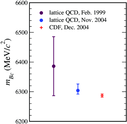
Figure 6: The lattice prediction for the mass of the $B_{c}$ meson has improved enormously from the old quenched calculation of 1999 to the new calculation that includes the effects of sea quarks. On the right is the experimental result that followed.

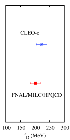
Figure 7: Lattice QCD result for the decay constant of the $D$ meson [9] compared to the result obtained by dividing the experimental value of the leptonic decay rate of the $D$ from CLEO-c by a previous result for $(V_{cd})^{2}$.

3.3 Weak decay rates for hadrons

Decay rates that can be accurately calculated for hadrons are those in which there is at most one hadron in the final state. Luckily a lot of the interesting decay modes caused by the weak force fall into this category. There are decay modes in which a quark and antiquark in a meson annihilate to a $W$ boson (obviously this requires the meson to have an electrical charge) that then decays to an electron and an antineutrino. This is known as a leptonic decay because the final products are all so-called leptons (particles that have no color charge and do not feel the strong force). There are also decay modes in which a quark or antiquark inside a hadron changes flavor and emits a $W$ boson. The meson therefore changes to another type and leptons are produced from the $W$. This is the analogue of nuclear $\beta$ decay and is known as semileptonic decay since there is one hadron, as well as leptons, in the final state.

As described in subsection 1.3 an element of the CKM matrix appears every time a $W$ boson is emitted by a quark. The rate for leptonic or semileptonic decays is then a product of the square of the appropriate CKM element, say $V_{ab}$, multiplied by the rate of the basic process in which the quark-antiquark annihilation occurs (for leptonic decay) or the quarks and antiquarks rearrange themselves (for semileptonic decay). This basic process takes place in a background of strongly interacting QCD radiation and so needs the techniques of lattice QCD for its calculation. Then to determine $V_{ab}$ we simply divide the experimentally determined actual rate by the lattice QCD calculation of the basic process, and take the square root. Luckily there is an example of decay mode of this kind for all the CKM elements in the first two rows of the matrix:

$$\left(\begin{array}[]{ccc}{\bf V_{ud}}&{\bf V_{us}}&{\bf V_{ub}}\\ \pi\rightarrow l\nu&K\rightarrow l\nu&B\rightarrow\pi l\nu\\ &K\rightarrow\pi l\nu&\\ {\bf V_{cd}}&{\bf V_{cs}}&{\bf V_{cb}}\\ D\rightarrow l\nu&D_{s}\rightarrow l\nu&B\rightarrow Dl\nu\\ D\rightarrow\pi l\nu&D\rightarrow Kl\nu&\\ {\bf V_{td}}&{\bf V_{ts}}&{\bf V_{tb}}\\ \langle B_{d}|\overline{B}_{d}\rangle&\langle B_{s}|\overline{B}_{s}\rangle&\\ \end{array}\right)$$

As described earlier, the determination of the CKM elements and tests of the self-consistency of the CKM matrix are a big part of the current experimental programme and lattice calculations of these leptonic and semileptonic processes will be a key factor in the precision with which this can be done. For the decay rates that will be used for CKM element determination it is important to have cross-checks against experiment of other similar decay rates as a confirmation of the systematic error analysis.

The CKM elements for $b$ quarks, $V_{ub}$ and $V_{cb}$, are the most poorly known. Lattice calculations are currently being done for the relevant leptonic and semileptonic decays for the mesons called $B$ mesons that contain a $b$ quark or antiquark and a $u$, $d$ or $s$ antiquark or quark respectively. These mesons are being studied extensively in the ‘$B$-factory’ experiments at SLAC and KEK in Japan and will be studied further in the LHCb experiment at CERN. A good test of these calculations is the equivalent calculation for $c$ quarks, since a lot of the understanding of systematic errors in the lattice calculations is similar. For $c$ quarks the CKM elements are well-known from other processes. This means that an experimental result for the leptonic decay rate of the equivalent of the $B$ meson called the $D$ meson can be used with a known value of $V_{cx}$ to determine the annihilation amplitude or ‘decay constant’, $f_{D}$, that can be directly calculated in lattice QCD. The CLEO-c collaboration have taken up the challenge of determining these leptonic rates for direct tests of the lattice calculations. Currently the situation is as in Figure 7 in which the lattice result [9] and the experimental result [10] have roughly 8% errors and agree within this precision. The experimental results will improve as the experiment runs for longer. The challenge for the lattice QCD theorists is to improve their discretisation of the QCD Lagrangian for charm quarks so that they can improve their prediction of $f_{D}$ to the few percent level ahead of precise experimental results. In fact this year the Belle collaboration, working at KEK in Japan, produced a first result for the leptonic decay rate of the $B$ meson [11]. In principle this can be used, along with a lattice calculation of $f_{B}$, to determine $V_{ub}$ but at present the experimental result is not accurate enough for this. It shows however, the possibilities that might exist in the future.

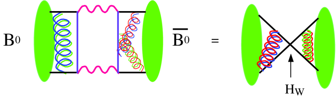
Figure 8: The ‘box’ diagram for the mixing of neutral $B$ mesons with their antimeson. On the right is the process that must be calculated in lattice QCD.

The lattice calculation of $f_{B}$ is important also for another reason - because it is the first stage on the way to calculating the oscillation rate for neutral $B$ mesons that will yield the CKM elements in the bottom row of the matrix, $V_{td}$ and $V_{ts}$. Neutral $B$ mesons have a meson and antimeson that can change into each other via a process dominated by the diagram shown in Figure 8 in which the $\overline{b}$ antiquark in the $B^{0}$ emits a $W$ and changes to $\overline{t}$ antiquark which annihilates with the $d$ quark so that another $W$ is created - the 2 $W$ bosons then convert back to a $b$ and a $\overline{d}$ which is the antimeson, $\overline{B}^{0}$. This means that the weak interactions mix the two states and, as these states propagate in time their identity fluctuates, rather like the way energy sloshes back and forth between two coupled pendulums. This oscillation can be picked up experimentally by studying the decay products from a $B^{0}$, $\overline{B}^{0}$ pair that are produced in a correlated way (e.g. from $e^{+}e^{-}$ annihilation at a $B$-factory). This year CDF have measured the oscillation rate for the neutral $B_{s}$ meson for the first time [13]. This is much harder to see, being more rapid, than the rate for the $B_{d}$ meson that has been known for some while.

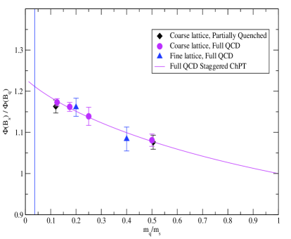
Figure 9: The ratio $f_{B_{s}}\sqrt{M_{B_{s}}}/f_{B}\sqrt{M_{B}}$ as a function of the light ($u/d$) quark mass, $m_{q}$ in units of $m_{s}$ from lattice QCD calculations including the effect of sea quarks [12]. The calculations have been done at light enough values of $m_{q}$ that it is now possible to extrapolate to the physical answer with only a small error.

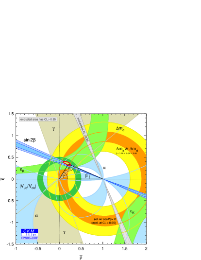
Figure 10: The current status of the search for the vertex of the ‘unitarity triangle’ that expresses the unitarity of the CKM matrix [14].

From Figure 8 it is clear that the oscillation rate will depend on the combination $V_{td}V^{*}_{tb}$ for the $B^{0}$ meson and $V_{ts}V^{*}_{tb}$ for the $B_{s}$ meson. The ratio will then yield $V_{ts}/V_{td}$ if the rates for the basic process are known, including the QCD effects. These can be calculated in lattice QCD from the righthand diagram of Figure 8 where the propagation of the heavy $W$ and $t$ quarks has been shrunk to an effective point interaction. This calculation is ongoing but the initial phase of it (which we believe may actually give a good approximation to the answer) is to calculate the ratio of the decay constants of the $B_{s}$ and $B^{0}$ (although neither can actually decay leptonically since they are neutral particles).

Lattice QCD calculations have now given an accurate result for $f_{B_{s}}/f_{B^{0}}$ of 1.20(3) [12]. Several sources of lattice QCD systematic error cancel in this ratio, making it a good quantity to study. The result is a significant improvement over previous calculations because the effects of sea quarks are included and results are available at very light values of $m_{u/d}$. Figure 10 shows the lattice results for several different values of $m_{u/d}$. It can be seen that there is significant dependence on this mass but that the extrapolation to get to the physical answer from the lightest points is now small.

The results for elements of the CKM matrix can be graphically represented as a search for the vertex of a triangle in the so-called ‘$\rho,\eta$’ plane where $\rho$ and $\eta$ are a parameterisation of the elements of the CKM matrix. The current situation from the CKMfitter group [14] is shown in Figure 10. The limits provided by the circles of $V_{ub}/V_{cb}$ and $\Delta m_{s}/\Delta m_{d}$ (the $B_{s}$ and $B^{0}$ oscillation rates) are very important to pinning down the vertex labelled by angle $\alpha$. The accuracy of these constraints is limited by the accuracy of the accompanying lattice QCD calculations at present [15, 16, 17]. The work currently underway, and described here, as well as that on semileptonic decay rates [18, 19], will be key to reducing the size of the blob in the Figure to the level where it provides a very serious test of the unitarity of the matrix and the self-consistency of the Standard Model.

4 Conclusions

Lattice QCD is entering a very exciting period as the first accurate calculations that include the effects of sea quarks reach maturity. The list of hadron masses and mass differences that agree with experiment at the few percent level continues to grow, the parameters of QCD have been determined with precision and a prediction for the mass of the $B_{c}$ successfully made. Work continues on the decay rates needed for the accurate determination, when combined with experiment, of the CKM matrix. There is plenty more to do in lattice QCD and doubtless there will be in Beyond the Standard Model physics when we find it!

I am grateful to the conference organisers for the opportunity to present this work to such an interesting audience and to my collaborators in the HPQCD and UKQCD collaborations.

References

References

- [1] S. Naik, Nucl. Phys. B316 238 (1989); D. Toussaint and K. Orginos [MILC collaboration], Nucl. Phys. Proc. Suppl. 73 909 (1999) [arXiv:hep-lat/9809148]; G. P. Lepage, Phys. Rev. D59 074502 (1999) [arXiv:hep-lat/9809157].
- [2] C. T. H. Davies et al [Fermilab, HPQCD, MILC, UKQCD Collaborations], Phys. Rev. Lett. 92 022001 (2004) [arXiv:hep-lat/0304004].
- [3] Q. Mason, H. D. Trottier, C. T. H. Davies, K. Foley, A. Gray, G. P. Lepage, M. Nobes, J. Shigemitsu, [HPQCD Collaboration], Phys. Rev. Lett. 95:052002 (2005) [arXiv:hep-lat/0503005].
- [4] Q. Mason, H. D. Trottier, R. Horgan, C. T. H. Davies, G. P. Lepage, [HPQCD Collaboration] Phys. Rev. D73:114501 (2006) [arXiv:hep-ph/0511160].
- [5] A. Gray, I. Allison, C. T. H. Davies, E. Gulez, G. P. Lepage, J. Shigemitsu, M. Wingate [HPQCD and UKQCD Collaborations], Phys. Rev. D72:094507 (2005) [arXiv:hep-lat/0507013].
- [6] M. Nobes, H. Trottier, PoS LAT2005:209 (2006) [arXiv:hep-lat/0509128].
- [7] I. F. Allison, C. T. H. Davies, A. Gray, A. S. Kronfeld, P. B. Mackenzie and J. N. Simone [HPQCD Collaboration], Phys. Rev. Lett. 94 172001 (2005) [arXiv:hep-lat/0411027].
- [8] D. Acosta et al [CDF Collaboration], Phys. Rev. Lett. 96:082002 (2006) [arXiv:hep-ex/0505076]; W. Wester for CDF, Nucl. Phys. B Proc. Suppl. 156:240 (2006).
- [9] C. Aubin et al [FNAL, MILC and HPQCD Collaborations], Phys. Rev. Lett. 95:122002 (2005) [arXiv:hep-lat/0506030].
- [10] M. Artuso et al [CLEO Collaboration], Phys. Rev. Lett. 95:251801 (2005) [arXiv:hep-ex/0508057].
- [11] K. Ikado for the the Belle Collaboration, Proceedings of FPCP 2006 [arXiv:hep-ex/0605068].
- [12] A. Gray, M. Wingate, C. T. H. Davies, E. Gulez, G. P. Lepage, Q. Mason, M. Nobes, J. Shigemitsu [HPQCD Collaboration], Phys. Rev. Lett. 95:212001 (2005)[arXiv:hep-lat/0507015]
- [13] G. Gomez-Caballos et al [CDF Collaboration], Proceedings of FPCP2006.
- [14] J. Charles et al [CKM fitter group], Eur. Phys. J. C41:1 (2005)[arXiv:hep-ph/0406184], updates at http://ckmfitter.in2p3.fr.
- [15] M. Okamoto, PoS LAT2005:013 (2006) [arXiv:hep-lat/0510113].
- [16] M. Wingate, Mod. Phys. Lett. A21:1167 (2006) [arXiv:hep-ph/0604254].
- [17] P. Mackenzie, Proceedings of FPCP2006 [arXiv:hep-ph/0606034].
- [18] E. Gulez, A. Gray, M. Wingate, C. T. H. Davies, G. P. Lepage, J. Shigemitsu, [HPQCD Collaboration] [arXiv:hep-lat/0601021].
- [19] C. Aubin et al [FNAL, MILC and HPQCD Collaborations], Phys. Rev. Lett. 94:011601 (2005) [arXiv:hep-ph/0408306].