Applications of Chiral Perturbation theory to lattice QCD

Abstract

These lectures describe the use of effective field theories to extrapolate results from the parameter region where numerical simulations of lattice QCD are possible to the physical parameters (physical quark masses, infinite volume, vanishing lattice spacing, etc.). After a brief introduction and overview, I discuss three topics: 1) Chiral perturbation theory ($\chi$PT) in the continuum; 2) The inclusion of discretization effects into $\chi$PT, focusing on the application to Wilson and twisted-mass lattice fermions; 3) Extending $\chi$PT to describe partially quenched QCD.

1 Overview and Aims

More than 30 years after Wilson introduced lattice QCD[1], and more than 25 years after Creutz’s pioneering numerical studies of non-abelian gauge theories[2], we can now simulate lattice QCD, including quarks, with parameters that approach their physical values. This is the result not only of advances in computer power but also of improvements in algorithms and actions. In particular, we can simulate QCD with pion masses of $250\;$MeV or lower, with the minimum value depending on the choice of fermion action. Such masses should allow a controlled extrapolation to the physical pion masses, one that can give errors at the few percent level[3]. One of the aims of the field is to provide results with this accuracy for many hadronic quantities, allowing both tests of the method and predictions for unmeasured quantities. This goal has begun to be attained[4].

Despite the successes just outlined, it is important to keep in mind the limitations of LQCD (lattice QCD). Simulations are, and will remain for the foreseeable future, limited in scope—one or two particle states in a box unlikely to exceed $L=3-5\;$fm, with lattice spacings unlikely to be smaller than $a\approx 0.05\;$fm, and pion masses unlikely to drop below $200\;$MeV. In order to connect these results to those for physical quark masses in the continuum and infinite volume limits one needs a quantitative theoretical understanding of how to extrapolate. Such an understanding can be provided by chiral perturbation theory generalized to include discretization errors, and is the topic of these lectures.

One way to think of this situation is that LQCD is a powerful tool with several adjustable parameters (“knobs”). While we are able to turn these knobs independently (unlike in the physical world where they are fixed), we cannot turn them to their physical values. Thus we are stuck simulating theories with unphysical values of the parameters, and we need additional theoretical input.

In fact, there are several other knobs (beyond quark masses, $a$, $L$ and $\alpha_{\rm EM}$) that we can adjust independently. We can use different sea and valence quark masses—giving partially quenched (PQ) theories—or we can go further and use different actions for valence and sea quarks—“mixed action” simulations. An interesting example of the latter is to use valence fermions with good chiral symmetry (Domain-Wall or Overlap) and cheaper sea quarks (staggered or Wilson-like). Both PQ and mixed action theories are “really” unphysical: they not only have unphysical values of the parameters but they are also not unitary. Nevertheless, they are well-defined Euclidean statistical systems, with long-distance correlations, and it is plausible that they can be described by an effective chiral theory. Furthermore, in both cases there are points in parameter space for which the theories are physical, which “anchor” the effective theories. I will discuss this in detail for PQQCD in sec. 4, and for now only illustrate the situation with Fig. 1. The aim is to use the freedom provided by having extra knobs, which are relatively cheap to turn, in order to improve the accuracy of the extrapolation to the physical point: “physical results from unphysical simulations”[6]. This is an essential feature of the MILC collaboration’s work on decay constants and quark masses[3].

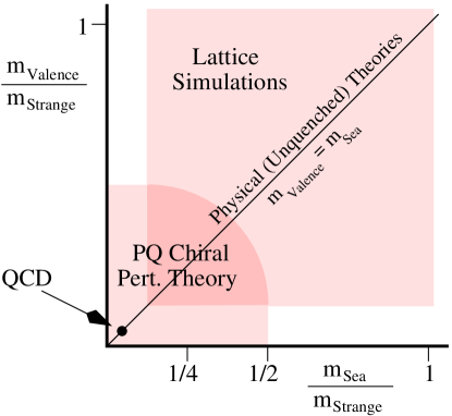
Figure 1: PQQCD: using $m_{\rm val}\neq m_{\rm sea}$ and PQ$\chi$PT to better extrapolate (from the overlap of the shaded regions) to the physical theory.

A different example of unphysical theories is the use of “rooted” staggered fermions. Each staggered flavor leads to four degenerate “tastes” in the continuum limit, and the standard approach to obtain a single continuum fermion per flavor is to take the fourth root of the fermion determinant. As the taste symmetry is broken for $a\neq 0$, this rooting leads, however, to a non-local single-flavor fermion action on the lattice[7]. The implications of a non-locality that formally vanishes as $a\to 0$ are controversial—does one remain in the universality class of QCD? I will not discuss this issue here, but only note that the theory at $a\neq 0$ is undoubtedly unphysical, and the chiral-continuum extrapolation can only be done if one has an effective theory which describes the unphysical features. This is provided by “(rooted) staggered $\chi$PT”[8, 9, 10]. Whatever the outcome of the rooting controversy, this is another example of using effective field theory to obtain physical results from unphysical simulations.

Due to limitations of time and space, I will discuss only a subset of applications of $\chi$PT to LQCD in these lectures. I begin with a brief introduction to $\chi$PT in the continuum, with an emphasis on lessons for the lattice. I follow that with the example of incorporating discretization errors into $\chi$PT for twisted-mass fermions, which includes Wilson and improved Wilson fermions as a subset. In this case the theory is physical, but gives a nice example of the power of adding an extra knob (the twist angle) and of the utility of $\chi$PT. Finally, I discuss PQ$\chi$PT, i.e. chiral perturbation theory for PQQCD.

I will mainly focus on the theoretical set-up and on general issues of the applicability of $\chi$PT. I will not provide a review of the status and accuracy of the state-of-the-art extrapolations. My hope is that this introduction to the tools will allow the reader to critically assess current work.

2 Review of $\chi$PT in the continuum

In this section I describe the construction of the chiral Lagrangian in the continuum. There are many good books and lectures on this topic. I have found those by Donoghue, Golowich & Holstein[11], Ecker[12], Georgi[13], Kaplan[14], Kronfeld[15], Manohar[16] and Pich[17] very useful.

2.1 Effective Field Theories in general

In these lectures I consider two examples of effective field theories (EFTs): $\chi$PT as an EFT for QCD, and Symanzik’s effective continuum theory for lattice QCD (the latter to be discussed in sec. 3.4). Thus it is useful to begin with a discussion of EFTs in general. If you are unfamiliar with the subject then some of this section may be hard to follow in detail, but my aim is to begin with a broad-brush sketch, which will be filled in later.

The generic situation is that we have an underlying theory in which there is a separation of scales. In the theories of interest we have:

$$\chi p_{\pi}\sim m_{\pi}\ll m_{\rho},m_{N}\,;$$PT: (1)

Symanzik: $$p_{\rm quark},p_{\rm gluon}\sim\Lambda_{\rm QCD}\ll\pi/a\,.$$ (2)

Note that in the former case there is a separation of masses, with the “pions” (by which I mean the light pseudoscalars: $\pi$, $K$ and $\eta$) being lighter than all other hadrons, while in Symanzik’s theory we choose to consider momenta much smaller than the lattice cut-off. In both cases there is a good reason to split off the low-scale physics. For $\chi$PT it is because the pion sector changes most rapidly as we approach the chiral limit (as we will see in detail). For Symanzik’s theory we want to understand the impact of lattice spacing errors on the quarks and gluons which dominate the non-perturbative contributions to hadronic quantities.

Crudely speaking, we now introduce a momentum cut-off $\Lambda$ lying between the two scales, and “integrate out” the high-momentum degrees of freedom. This process is illustrated schematically in Fig. 2. It leaves only pions with low momenta in $\chi$PT, and continuum-like quarks and gluons in the Symanzik theory. These degrees of freedom interact via vertices that are quasi-local, with a physical size $\Lambda^{-1}$. This quasi-locality follows because we consider only external momenta satisfying $p\ll\Lambda$, so the high-momentum degrees of freedom are always highly virtual. The vertices are then expanded in powers of $p/\Lambda$, yielding local operators with increasing numbers of derivatives. The low-momentum modes themselves can become nearly on shell (or exactly on shell if we continue to Minkowski space), but the resulting analytic structure of correlation functions (leading to cuts in Minkowski space) is maintained in the effective theory.

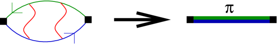
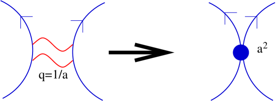
Figure 2: Generation of effective field theories.

This description is impractical to implement in most cases. In particular, we do not know how to integrate out quarks and gluons from QCD analytically to yield a theory of pions, since confinement is a non-perturbative phenomenon. Even in the Symanzik theory, where one might have expected that quarks and gluons with $p\sim\pi/a$ would have been perturbative since $1/a\mathrel{\hbox to0.0pt{\lower 3.0pt\hbox{$\mathchar 536\relax$}\hss}\raise 2.0pt\hbox{$\mathchar 318\relax$}}2\;$GeV ($a\mathrel{\hbox to0.0pt{\lower 3.0pt\hbox{$\mathchar 536\relax$}\hss}\raise 2.0pt\hbox{$\mathchar 316\relax$}}0.1\;$fm), it turns out that accurate results mostly require non-perturbative calculations. The beauty of the EFT method, however, is that we do not actually need to do the integrations. Instead, following Weinberg[18] we can rely on the general properties of EFTs. If the underlying theory is physical, its S-matrix will be unitary, Lorentz-invariant, satisfy cluster decomposition, and transform appropriately under the internal symmetries. These properties must be maintained by the EFT, which is, after all, designed to reproduce the S-matrix of the low-momentum degrees of freedom. The only known way to do this is with a local, Lorentz-invariant Lagrangian. It should be constructed solely from the low-energy degrees of freedom, and satisfy the same internal symmetries as the underlying theory. All possible terms consistent with these symmetries must be included—this precludes the need to explicitly integrate-out degrees of freedom, at the price of introducing unknown constants.

One notable feature of the resulting $\mathcal{L}_{\rm eff}$ is that it is not renormalizable, and thus valid only over a limited energy range. This is an intrinsic part of the construction: we know that the EFT breaks down when $p\mathrel{\hbox to0.0pt{\lower 3.0pt\hbox{$\mathchar 536\relax$}\hss}\raise 2.0pt\hbox{$\mathchar 318\relax$}}\Lambda$. Non-renormalizability does not, however, imply a lack of calculability. As we will see, one can expand quantities in powers of $p/\Lambda$, with a finite number of unknown coefficients at each order. The limitations of the method are then (a) the need to introduce unknown coefficients and (b) an unavoidable truncation error. This error, however, decreases as the separation in scales increases (i.e. as $m_{\pi}\to 0$ or $a\to 0$).

As just described, the justification of EFT is based on properties of the S-matrix, and thus rooted in Minkowski space. While this is fine for the development of continuum $\chi$PT (my first topic), the natural objects in lattice simulations (my second topic) are Euclidean (finite-volume) correlation functions of local operators. In particular, the discretization errors are constrained by the symmetries of a Euclidean lattice. Thus an alternative approach to developing and justifying an EFT is needed. This has been provided for the case at hand by Symanik[20], using an extension of renormalization theory. The result (established to all orders in perturbation theory) is that the recipe given above still applies: keep all local terms consistent with the symmetries of the underlying theory (in this case the discrete symmetries of a Euclidean lattice). My third topic, PQQCD, is also strictly limited to Euclidean space, but here neither of the previous justifications apply, and one must make further assumptions.

Because my second and third topics involve Euclidean theories, I have chosen to couch the discussion of the first ($\chi$PT) also in Euclidean space. This allows later sections to build on the earlier notation. In fact, it is perfectly legitimate, having determined the Minkowski-invariant local effective Lagrangian, to rotate this to Euclidean space. The result will be the most general Euclidean-invariant local Lagrangian (consistent with the other symmetries, which are unaffected by the rotation). This Lagrangian will reside in the functional integral which generates the Euclidean correlation functions of the theory.

2.2 Chiral symmetry in QCD and its breaking

Without further ado, let me turn to the first concrete example, $\chi$PT. The fermionic part of Euclidean Lagrangian for QCD is given by

$${\mathcal{L}}_{QCD}=\overline{Q}_{L}{\rm D}\!\!\!\!/\,Q_{L}+\overline{Q}_{R}{\rm D}\!\!\!\!/\,Q_{R}+\overline{Q}_{L}MQ_{R}+\overline{Q}_{R}M^{\dagger}Q_{L}\,.$$ (3)

where I have included only the $N=3$ light quarks, $Q^{tr}=(u,d,s)$, $\overline{Q}=(\overline{u},\overline{d},\overline{s})$. I will also consider the $N=2$ theory without the strange quark. Left- and right-handed fields are defined with projectors $P_{\pm}=(1\pm\gamma_{5})/2$, and are $Q_{L,R}=P_{\mp}Q_{L,R}$ and $\overline{Q}_{L,R}=\overline{Q}_{L,R}P_{\pm}$. There is no problem with $\overline{Q}_{L}$ and $Q_{L}$ being defined with the different projectors, since $\overline{Q}$ and $Q$ are independent fields. The key fact is that, in the massless limit, left- and right-handed quarks can be rotated independently, so the Lagrangian has a ${G}=SU(3)_{L}\times SU(3)_{R}$ chiral symmetry under which

$$Q_{L,R}\to U_{L,R}Q_{L,R}\,,\quad\overline{Q}_{L,R}\to\overline{Q}_{L,R}U_{L,R}^{\dagger}\,:\quad U_{L,R}\in SU(3)_{L,R}\,.$$ (4)

There is also the overall vector $U(1)$ symmetry, which counts quark number, while the apparent axial $U(1)$ symmetry is broken by the anomaly.

Quark masses enter through the mass matrix $M$, which is conventionally taken to be $M=\textrm{diag}(m_{u},m_{d},m_{s})=M^{\dagger}$. These masses break the chiral symmetry: any non-zero values violate the axial symmetries (those with $U_{L}=U_{R}^{\dagger}$), while the vector symmetries ($U_{L}=U_{R}$) are broken unless the masses are degenerate. We can, however, formally retain the chiral symmetry of $\mathcal{L}_{QCD}$ by treating $M$ as a complex “spurion field” transforming as $M\to U_{L}MU_{R}^{\dagger}$ and $M^{\dagger}\to U_{R}M^{\dagger}U_{L}$. This is a convenient trick for keeping track of the symmetry-breaking caused by the mass term.

Since chiral symmetry is key to all that follows, and quark masses break this symmetry, we must require that $M$ be small. What does small mean? One criterion is that $M$ should be small compared to the QCD scale, $m_{q}\ll\Lambda_{QCD}\sim 300\;$MeV. A more precise criterion will arise from $\chi$PT: $m_{\pi,K,\eta}\ll\Lambda_{\chi}\equiv 4\pi f_{\pi}\approx 1200\;$MeV. It follows that in physical QCD, with $(m_{u}\!+\!m_{d})/2\approx 4\;$MeV, $SU(2)_{L}\times SU(2)_{R}$ is a very good approximate symmetry, while $SU(3)_{L}\times SU(3)_{R}$ is more badly broken since $m_{s}\approx 100\;$MeV and $m_{K,\eta}\approx\Lambda_{\chi}/2$. This brings up an important question for lattice applications of $\chi$PT: can approximate chiral symmetry can be used to determine the strange quark mass dependence when $m_{s}^{\textrm{lat}}\approx m_{s}$? If not, then we can only use chiral symmetry to guide extrapolations in $m_{u}$ and $m_{d}$.

Chiral perturbation theory is an expansion about the chiral limit, $M=0$, so I first discuss massless QCD. It is expected in this theory that the exact chiral symmetry is spontaneously broken by the vacuum. This is based on an accumulation of evidence about QCD itself: the lightness of the $\pi$, $K$ and $\eta$ are consistent with their being pseudo-Nambu-Goldstone bosons (PGBs) of the broken approximate chiral symmetry of real QCD; the absence of (approximate) parity-doubling in the hadron spectrum, e.g. $m_{N}(P=+)\neq m_{N}(P=-)$, as would be required by an unbroken (approximate) chiral symmetry; and the accumulated successes of $\chi$PT, especially in the $SU(2)$ sector. It is also expected that the order parameter for chiral symmetry breaking is the condensate:

$$\langle\overline{q}q\rangle=\langle(\overline{q}_{L}q_{R}+\overline{q}_{R}q_{L})\rangle\sim\Lambda_{\rm QCD}^{3}\neq 0\,,\quad q=u,d,s\,.$$ (5)

The vector symmetry is not expected to be spontaneously broken, based on the presence of approximate $SU(3)_{V}$ multiplets in the hadron spectrum, and on theoretical considerations[23]. This implies that the condensates are equal in the massless theory, $\langle\overline{u}u\rangle=\langle\overline{d}d\rangle=\langle\overline{s}s\rangle$.

The form of the condensate in eq. (5) is a convention. There is in fact a manifold of equivalent vacua related by chiral transformations, and parameterized by the orientation of the condensate in flavor space:

$$\Omega_{ij}=\langle Q_{L,i,\alpha,c}\overline{Q}_{R,j,\alpha,c}\rangle\ {\lower 2.58334pt\hbox{$\stackrel{{\scriptstyle G}}{{\longrightarrow}}$}}\ U_{L}\,\Omega\,U_{R}^{\dagger}\,.$$ (6)

Here I have shown the summed Dirac and color indices explicitly ($\alpha$ and $c$, respectively), since $Q$ and $\overline{Q}$ are in the opposite order from usual. This order makes the flavor matrix structure (indices $i$ and $j$) transparent, and is particularly useful when discussing PQ$\chi$PT below. The assumption of unbroken vector symmetry implies that $\Omega_{ij}=\omega\,\delta_{ij}$ must lie in the manifold, and so the general point is $\omega U_{L}U_{R}^{\dagger}$. In this language, chiral symmetry breaking is equivalent to $\omega$ being non-zero, for then the vacuum is left invariant only by a subgroup $H$ of $G$:

$$\underbrace{SU(3)_{L}\times SU(3)_{R}}_{{G}}\longrightarrow\underbrace{SU(3)}_{{H}}\,,$$ (7)

The nature of $H$ is simplest using the conventional vacuum orientation, $\Omega_{ij}=\omega\,\delta_{ij}$, with $\omega=-\langle\overline{q}q\rangle$. Then $H=SU(3)_{V}$ (with $U_{L}=U_{R}$), while the axial transformations with $U_{L}=U_{R}^{\dagger}$ are broken ($\Omega=\omega\to\omega U_{L}^{2}$).

Goldstone’s theorem then implies that there are 8 massless Nambu-Goldstone bosons (NGB—labeled $\pi^{b}$, and corresponding to the $\pi$, $K$, and $\eta$), each coupled to one of the eight broken axial generators. For the conventional vacuum orientation, one has

$$\langle\pi^{b}(p)|\overline{Q}\gamma_{\mu}\gamma_{5}T^{a}Q(0)|0\rangle=-if_{\pi}p_{\mu}\delta^{ba}\,,$$ (8)

with $T^{a}$ being $SU(3)$ generators. The masslessness of the NGB follows from the fact that rotations of the condensate with four-momentum $p$ cost zero energy as $p\to 0$, in which limit they become global rotations.

We now have the ingredients with which to construct an EFT: a separation of scales ($m_{\rm GB}=0$ compared to the scale of other hadron masses—$m_{\rho}$, $m_{\eta}^{\prime}$, $m_{\rm proton}$, etc., with $m_{\rm had}\approx 1\;$GeV), and a knowledge of the symmetries of the underlying theory. The EFT will contain only NGB as dynamical degrees of freedom, and should be valid as long as $p_{\rm GB}\ll m_{\rm had}$. The spurion field $M$ should also be added to include the effects of quark masses.

Representing NGB fields is probably the most conceptually non-trivial step of the construction, because (a) the underlying theory is written in terms of quarks rather than mesons (one is not just “thinning” degrees of freedom, one is also changing basis) and (b) the choice is not unique[24, 25]. Because of point (b), the strategy is simply to find any representation which works—it turns out that by field redefinitions one can then switch to other choices as desired.

Since there are no precise rules to follow, it is useful to proceed by analogy. To this end, I recall the canonical example of spontaneous symmetry breaking: a complex scalar field with a “Mexican hat” potential

$$V=-\mu^{2}\phi^{\dagger}\phi+{\lambda}(\phi^{\dagger}\phi)^{2}/2\,.$$ (9)

There is a $G=U(1)$ phase symmetry, $\phi\to e^{i\alpha}\phi$, which is spontaneously broken if $\mu^{2}>0$, for then there is a non-zero vacuum expectation value (VEV) $|\langle\phi\rangle|=v=\sqrt{\mu^{2}/\lambda}$. The vacuum manifold consists of the phase of $\langle\phi\rangle$, and is thus $U(1)$. The symmetry breaking is ${G}\longrightarrow{H}=1$, implying a single NGB corresponding to phase rotations. The EFT for this massless mode is analogous to that we wish to write down for the pions in QCD.

The advantage of this theory, compared to QCD, is that we can directly construct the EFT by integrating out heavy fields, as long as $\lambda$ is small enough that we can use perturbation theory. Having done so, we can see how the EFT could be obtained using the symmetries alone, and use this to guide the construction for QCD.

I decompose the field in a way which differs from that used, say, in studying the Higgs: $\phi(x)=ve^{\rho(x)}e^{i\theta(x)}$ rather than $\phi(x)=v+h(x)$. This choice picks out the NGB degree of freedom, $\theta$, explicitly, and allows the phase symmetry to act linearly: $e^{i\theta[x]}\to e^{i\alpha}e^{i\theta[x]}$. If we integrate out the heavy radial degree of freedom, $\rho$, we obtain an effective Lagrangian in terms of $e^{i\theta}$. But we do not need to do any work to determine the general form of $\mathcal{L}_{\rm eff}$—we need only require locality, reality, Euclidean and $U(1)$ invariance. The result is

$$\mathcal{L}_{\rm eff}=c_{2}\partial_{\mu}(e^{i\theta})\partial_{\mu}(e^{-i\theta})+c_{4}\partial_{\mu}(e^{i\theta})\partial_{\mu}(e^{-i\theta})\partial_{\nu}(e^{i\theta})\partial_{\nu}(e^{-i\theta})+\dots\,,$$ (10)

where $c_{i}$ are unknown constants. Terms without derivatives on every factor of $e^{\pm i\theta}$ can be brought into the form shown (up to total derivatives) using $e^{i\theta}e^{-i\theta}=1$ and the abelian nature of the group. The result is a massless NGB having interactions proportional to $p^{4}$. It is an interesting exercise to check the latter result in perturbation theory using the conventional expansion in terms of $h(x)$—the $p^{4}$ arises from cancellations between non-derivative interactions.

We learn two things from the $U(1)$ example. First, to use the exponential of the “pion” fields, since it transforms linearly under $G$, and simplifies the implementation of the symmetries. Second, that a “fixed radius” form ($|e^{i\theta}|=1$ above) automatically includes only the NGB, excludes heavy degrees of freedom, and enforces the spontaneous breakdown of the symmetry (i.e. $U(1)$ is broken for any value of $\langle\theta\rangle$).

The QCD analog of $\langle\phi\rangle$ is the condensate $\Omega_{ij}$ of eq. (6)—both map out the corresponding vacuum manifolds. The analog of fixed length angular fluctuations is obtained by promoting $\Omega/\omega$ to a dynamical field $\Sigma_{ij}(x)$, corresponding roughly to fluctuations in the condensate. Just as $\Omega/\omega$ is in $SU(3)$, so is $\Sigma$, and the chiral transformation properties are the same:

$$\Sigma(x)\in SU(3):\qquad\Sigma(x)\ {\lower 2.58334pt\hbox{$\stackrel{{\scriptstyle G}}{{\longrightarrow}}$}}\ U_{L}\Sigma(x)U_{R}^{\dagger}\,.$$ (11)

Any VEV of $\Sigma$ breaks ${G}$ to ${H}=SU(3)$, leading to the desired number of NGBs. The fixed radius of $\Sigma$ (i.e. $\Sigma\Sigma^{\dagger}=\Sigma^{\dagger}\Sigma=1$) implies that the only degrees of freedom in $\Sigma$ are the NGBs. For example, if $\langle\Sigma\rangle=1$ we can expand as

$$\Sigma(x)=\exp\left(2i\Pi(x)/f\right)=\exp\left(2i\pi^{a}(x)T^{a}/f\right)\,,\qquad a=1,8,$$ (12)

in terms of the eight “pion” fields and a constant $f$ to balance dimensions. Note that although $\Sigma$ transforms linearly, this is not the case for the pion fields (e.g. $\delta\pi_{a}$ contains terms with any odd powers of $\pi_{b}$). Thus constructing $\mathcal{L}_{\rm eff}$ in terms of the pion field directly would be very difficult.

2.3 Constructing the pionic effective Lagrangian[26]

2.3.1 Building blocks for $\mathcal{L}_{\rm eff}$

We are now in business. The ingredients are $\Sigma$ and $\Sigma^{\dagger}$, as well as the spurions $M$ and $M^{\dagger}$. I recall their transformation properties under the chiral symmetry group $G=SU(3)_{L}\times SU(3)_{R}$:

$$\Sigma\to U_{L}\Sigma U_{R}^{\dagger}\,,\ \ \Sigma^{\dagger}\to U_{R}\Sigma^{\dagger}U_{L}^{\dagger}\,,\ \ M\to U_{L}MU_{R}^{\dagger}\,,\ \ M^{\dagger}\to U_{R}M^{\dagger}U_{R}^{\dagger}\,.$$ (13)

It is useful to construct objects which transform solely under the left-handed (LH) or right-handed (RH) sub-groups (and which I call respectively LH and RH building blocks), since they simplify enumeration of operators:

• ${L_{\mu}}=\Sigma\partial_{\mu}\Sigma^{\dagger}=-\partial_{\mu}\Sigma\Sigma^{\dagger}={-L_{\mu}^{\dagger}}\longrightarrow U_{L}{L_{\mu}}U_{L}^{\dagger}$

• $M\Sigma^{\dagger}\longrightarrow U_{L}{(M\Sigma^{\dagger})}U_{L}^{\dagger}\,,\qquad{\Sigma M^{\dagger}}\longrightarrow U_{L}{(\Sigma M^{\dagger})}U_{L}^{\dagger}$

• ${R_{\mu}}=\Sigma^{\dagger}\partial_{\mu}\Sigma=-\partial_{\mu}\Sigma^{\dagger}\Sigma={-R_{\mu}^{\dagger}}\longrightarrow U_{R}{R_{\mu}}U_{R}^{\dagger}$

• ${M^{\dagger}\Sigma}\longrightarrow U_{R}{(M^{\dagger}\Sigma)}U_{R}^{\dagger}\,,\qquad{\Sigma^{\dagger}M}\longrightarrow U_{R}{(\Sigma^{\dagger}M)}U_{R}^{\dagger}$ .

where I have repeatedly used the unitarity of $\Sigma$. From the fact that $\textrm{det}(\Sigma)=1$ one learns that $L_{\mu}$ and $R_{\mu}$ are traceless, e.g.

$$0=\partial_{\mu}(\det\Sigma)=\partial_{\mu}(\exp{\rm tr}\ln\Sigma)=\det\Sigma\ {\rm tr}(\partial_{\mu}\Sigma\Sigma^{-1})=-{\rm tr}({L_{\mu}})\,.$$ (14)

Thus $L_{\mu}$ and $R_{\mu}$ (“Weyl derivatives”) are elements of the Lie algebra, $su(3)$.

Another symmetry of QCD is parity. Since $\Sigma\sim q_{L}\overline{q}_{R}$ and $\Sigma^{\dagger}\sim q_{R}\overline{q}_{L}$, the transformations in the EFT are [with $x_{P}=(-\vec{x},x_{4})$]

$$\Sigma(x)\leftrightarrow\Sigma^{\dagger}(x_{P}),\ \ M\leftrightarrow M^{\dagger},\ \ L_{i}(x)\leftrightarrow-R_{i}(x_{P}),\ \ L_{4}(x)\leftrightarrow R_{4}(x_{P}).$$ (15)

If one expands about $\langle\Sigma\rangle=1$, as in eq. (12), then the pion field transforms as $\Pi(x)\to-\Pi(x_{P})$. There are also $C$ and $T$ symmetries, which I do not show explicitly.

I now enumerate terms which are local, real and satisfy the symmetries of QCD. These are just products of the building blocks above, with LH and RH blocks combined separately into traces to make them invariant under $G$. In fact, for the terms I display, one need only use LH building blocks as the results equal their “parity conjugates” (p.c.). Since in the end we expand in powers of momenta, it is useful to classify terms according to the number of derivatives. Similarly, as $M$ is treated as small, one should classify according to the number of spurion insertions. We will see that one should usually count two derivatives for each spurion.

There are no non-trivial terms without derivatives or spurions: these would be constructed from ${\rm tr}[(\Sigma\Sigma^{\dagger})^{n}]$ or powers or $\det\Sigma$, but both are constants. Euclidean invariance rules out a single derivative. The only independent term with two derivatives is

1. ${\rm tr}(L_{\mu}L_{\mu})=-{\rm tr}(\partial_{\mu}\Sigma\partial_{\mu}\Sigma^{\dagger})={\rm tr}(R_{\mu}R_{\mu})$,

while the only term with no derivatives and one mass insertion is

1. ${\rm tr}(M\Sigma^{\dagger})+{\rm tr}(\Sigma M^{\dagger})$ .

There are five terms with four derivatives:

1. $\left[{\rm tr}(L_{\mu}L_{\mu})\right]^{2}$

2. ${\rm tr}(L_{\mu}L_{\nu}){\rm tr}(L_{\mu}L_{\nu})$

3. ${\rm tr}(L_{\mu}L_{\mu}L_{\nu}L_{\nu})$ [not independent for two light flavors]]

4. ${\rm tr}(L_{\mu}L_{\nu}L_{\mu}L_{\nu})$ [not independent for 2 or 3 light flavors]]

5. The Wess-Zumino-Witten (WZW) term involving $\epsilon_{\mu\nu\rho\sigma}$[27] ;

two terms with two derivatives and one mass insertion:

1. ${\rm tr}(L_{\mu}L_{\mu})\ {\rm tr}(M\Sigma^{\dagger}+\Sigma M^{\dagger})$

2. ${\rm tr}(L_{\mu}L_{\mu}[M\Sigma^{\dagger}+\Sigma M^{\dagger}])$ ;

and three terms with two mass insertions:

1. $\left[{\rm tr}(M\Sigma^{\dagger}+\Sigma M^{\dagger})\right]^{2}$

2. $\left[{\rm tr}(M\Sigma^{\dagger}-\Sigma M^{\dagger})\right]^{2}$

3. ${\rm tr}(M\Sigma^{\dagger}M\Sigma^{\dagger}+M^{\dagger}\Sigma M^{\dagger}\Sigma)$ .

Each of these terms appears in $L_{\rm eff}$ with an independent unknown coefficient, except for terms 5 and 6 which, as noted, are not independent for certain chiral groups. I will not discuss the interesting structure of the WZW term, as it is complicated, and does not contribute to the simple processes considered here. I will also not continue the enumeration beyond this point. This has been done as part of next-to-next-to-leading order (NNLO) calculations[28], but is beyond the scope of this introduction.

With the enumeration of operators in hand, I turn to the predictions. I will assume a power counting with $\partial^{2}\sim M$ and justify this a posteriori. At leading order (LO) we have (the superscript on $\mathcal{L}$ counting derivatives):

$$\mathcal{L}^{(2)}_{\chi}=\frac{f^{2}}{4}{\rm tr}\left(\partial_{\mu}\Sigma\partial_{\mu}\Sigma^{\dagger}\right)-\frac{f^{2}B_{0}}{2}{\rm tr}(M\Sigma^{\dagger}+\Sigma M^{\dagger})\,,$$ (16)

where the unknown “low energy constants” (LECs) have been given their standard names $f$ and $B_{0}$. Since we are expanding about massless QCD, the only scale that can appear is $\Lambda_{\rm QCD}$, so we expect $f\sim B_{0}\sim\Lambda_{\rm QCD}$. Up to this stage, $M$ is a complex spurion field. To include the effects of quark masses we set it to its physical value: $M\to M_{0}=\textrm{diag}(m_{u},m_{d},m_{s})=M_{0}^{\dagger}$. This makes the potential—the second term in eq. (16)—depend on the direction of $\Sigma$, and we must determine its VEV by minimizing this potential. In other words, the quark masses, which break the chiral symmetry, pick out a preferred direction in the vacuum manifold. If all quark masses can be chosen positive (as is apparently the case in reality), then one finds that the VEV is $\langle\Sigma\rangle=1$. I stress that this result is convention dependent: we could choose $M=U_{L}M_{0}U_{R}^{\dagger}$, in which case $\langle\Sigma\rangle=U_{L}U_{R}^{\dagger}$.

2.3.2 Brief aside on vacuum structure

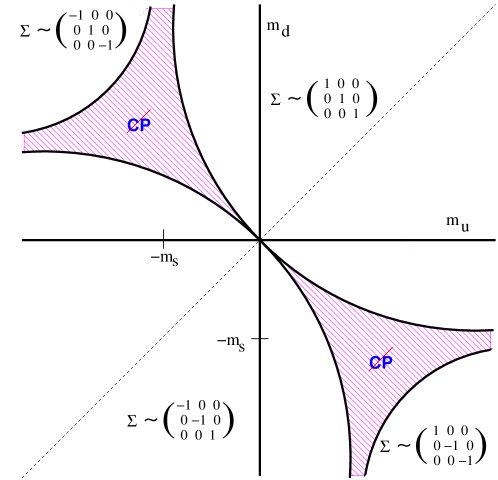
Figure 3: Phase structure at LO with 3 flavors and fixed $m_{s}$ (from Creutz[29]).

It is instructive to consider the vacuum structure of two flavor theory in a little more detail. Then we can write $\Sigma=\exp(i\theta\vec{n}\cdot\vec{\tau})$, implying $\Sigma+\Sigma^{\dagger}=2\cos\theta\times 1$, and thus ${V}^{(2)}\propto-{\rm tr}(M)\cos\theta$. This is minimized by $\langle\Sigma\rangle=1$ if ${\rm tr}M>0$, and by $\langle\Sigma\rangle=-1$ if ${\rm tr}M<0$. Note that at LO all that matters is the average quark mass ${\rm tr}M/2$; the difference $m_{u}-m_{d}$ does not enter. There is a first order phase transition when ${\rm tr}M$ changes sign at which the condensate flips sign but maintains its magnitude. Note, however, that the physical theory is the same for both signs of ${\rm tr}M$: one can go between them with a chiral rotation satisfying $U_{L}U_{R}^{\dagger}=-1$. I will discuss how discretization errors effect this transition in sec. 3.9 below.

With three flavors (or any odd number), the situation is more complicated because $\Sigma=-1$ is not an element of $SU(3)$. Changing the sign of $M$ leads to a different theory (one with the original $M$ plus a $\theta-$term with $\theta=\pi$). Without going into details, I show in Fig. 3 the phase structure if $m_{s}$ is fixed and positive while the other two masses change. The shaded region is where CP is spontaneously broken. In the real world we are very likely in the right-hand upper quadrant, but it is striking that such interesting physics lurks not far away and is contained in the LO potential.

2.3.3 Properties of pseudo-Nambu-Goldstone bosons at leading order

Assuming positive quark masses so that $\langle\Sigma\rangle=1$, we can study pion properties by inserting eq. (12) into $\mathcal{L}^{(2)}$ and expanding:

$$\mathcal{L}^{(2)}_{\chi} = {\rm tr}(\partial_{\mu}\Pi\partial_{\mu}\Pi)+\frac{1}{3f^{2}}{\rm tr}([\Pi,\partial_{\mu}\Pi][\Pi,\partial_{\mu}\Pi])+O([\partial\Pi]^{2}\Pi^{4})$$ (17)

$$\ \ +2B_{0}\;{\rm tr}(M\Pi^{2})-\frac{2B_{0}}{3f^{2}}{\rm tr}(M\Pi^{4})+O(M\Pi^{6}).$$

We can now understand the choice of factors multiplying the kinetic term in (16): they are chosen so that the pion kinetic term is correctly normalized [using ${\rm tr}(T^{a}T^{b})=\delta^{ab}/2$]. If $M=0$ [the first line of (17)], the pions are massless as required by Goldstone’s theorem, and their interactions all involve derivatives, as exemplified by $(\partial\Pi)^{2}\Pi^{2}$ term shown. Note that the non-abelian nature of the group allows there to be interaction terms with two (as opposed to four) derivatives, in contrast to the $U(1)$ example described above. This interaction term is non-renormalizable, as are subsequent terms involving more pion fields, with the dimensions balanced by factors of $f$.

Including $M$, the pions become massive pseudo-Goldstone bosons (PGB). $\chi$PT predicts at LO that the pion mass squared is proportional to the quark mass. The explicit form is simplest for degenerate quarks: $m_{\pi}^{2}=2B_{0}m_{q}$. This answers the following potential puzzle: how can physical quantities like $m_{\pi}^{2}$ be related to scheme- and scale-dependent quantities like $m_{q}$? The answer is that $B_{0}$ cancels the scheme dependence in $m_{q}$. This works for all the terms in the second line of (17), as they contain the common factor $B_{0}M$. For this reason it is useful to give the combination a name, specifically $\chi_{q}=2B_{0}m_{q}$.

The spurion terms also give rise to higher-order, non-renormalizable interactions among pions. Note that all vertices in $\mathcal{L}^{(2)}$ contain an even number of pions, because $\mathcal{L}^{(2)}$ is invariant under $\Pi(x)\leftrightarrow-\Pi(x)$. This is an accidental symmetry, which does not correspond to a symmetry of QCD (note that it differs from parity), and is broken by NLO terms in $\chi$PT. More precisely, it is broken by the WZW term, which allows, for example, interactions between five PGB.

LO $\chi$PT makes a number of predictions. First, it is clear that once $f$ and $\chi$ have been determined (e.g. from PGB masses and scattering amplitudes), all higher order vertices are predicted. But there are also predictions from the structure of the quadratic and quartic interactions alone. The former give relations between PGB masses, that latter between pion scattering in different channels (e.g. $I=0,1,2$ in the two-flavor theory). I will discuss the mass relations here.

First we need to place the physical particles in the pion matrix $\Pi$. This can be done using the vector symmetry corresponding to diagonal phase rotations, $U(1)_{V,u}\times U(1)_{V,d}\times U(1)_{V,s}\in U(3)_{V}$, which is unbroken by quark masses, and under which the pion field transforms linearly: $\Pi\to U_{V}\Pi U_{V}^{\dagger}$. The $\pi^{\pm}$, $K^{\pm}$, $K^{0}$ and $\overline{K^{0}}$ are charged under these symmetries (e.g. the $\pi^{+}$ has u-ness $+1$ and d-ness $-1$), and so live in definite off-diagonal positions in $\Pi$. Isospin then determines the position of the $\pi_{0}$, and orthogonality that of the $\eta$. Including normalizations, the result is

$$\Pi=\left(\begin{array}[]{ccc}\frac{\pi^{0}}{2}+\frac{\eta}{\sqrt{12}}&\frac{\pi^{+}}{\sqrt{2}}&\frac{K^{+}}{\sqrt{2}}\\ \frac{\pi^{-}}{\sqrt{2}}&-\frac{\pi^{0}}{\sqrt{2}}+\frac{\eta}{\sqrt{12}}&\frac{K^{0}}{\sqrt{2}}\\ \frac{K^{-}}{\sqrt{2}}&\frac{\overline{K^{0}}}{\sqrt{2}}&-\frac{2\eta}{\sqrt{12}}\end{array}\right).$$ (18)

Inserting this into $-2B_{0}{\rm tr}(M\pi^{2})$, we find that charged particle masses are proportional to the average mass of the quarks they contain: $m_{q_{i}q_{j}}^{2}=B_{0}(m_{i}+m_{j})$, $i\neq j$. While there are no predictions (masses of three pairs of CPT conjugate mesons are given in terms of three quark masses), one can determine quark mass ratios from the experimental PGB masses, e.g.

$$\frac{m_{K^{+}}^{2}+m_{K^{0}}^{2}}{2m_{\pi^{+}}^{2}}=\frac{m_{\ell}+m_{s}}{2m_{\ell}}\approx 13\qquad\left(m_{\ell}=\frac{m_{u}+m_{d}}{2}\right)\,.$$ (19)

This implies $m_{s}/m_{\ell}\approx 25$, up to NLO $\chi$PT and electromagnetic (EM) corrections. This is how we know that the strange quark is so much heavier than the up and down quarks. The corresponding determination of $(m_{u}-m_{d})/m_{\ell}$ (or equivalently $m_{u}/m_{d}$) from $(m_{K^{+}}^{2}-m_{K^{0}}^{2})/m_{\pi^{+}}^{2}$ fails, however, since the NLO corrections ($\Delta(m_{u}/m_{d})\propto m_{s}/\Lambda_{\rm QCD}$[30]) and EM contributions are potentially as large as the LO term in $\chi$PT. A determination of $m_{u}/m_{d}$ can be achieved by a direct lattice calculation of the meson masses using non-degenerate quarks together with an estimate of the EM contributions. The most accurate results at present[3] are $m_{u}/m_{d}=0.43(8)$ and $m_{s}/m_{\ell}=27.4(4)$.

The first predictions of $\chi$PT occur in the neutral sector. The $\pi^{0}$ and $\eta$ mix, but with an angle $\theta\sim(m_{u}-m_{d})/m_{s}$ that (despite the uncertainty in $m_{u}/m_{d}$) we know to be very small. Thus

$$m_{\pi^{0}}^{2} = m_{\pi^{+}}^{2}+O(\theta^{2}m_{K}^{2})+\dots\,,$$ (20)

$$\underbrace{m_{\eta}^{2}}_{(548\ \textrm{MeV})^{2}} = \underbrace{(2[m_{K^{+}}^{2}+m_{K^{0}}^{2}]-m_{\pi^{+}}^{2})/3}_{(566\ \textrm{MeV})^{2}}+O(\theta^{2}m_{K}^{2})+\dots\,.$$ (21)

Both predictions are well satisfied. The first, that of approximate isospin symmetry for the pions, holds not because $m_{u}/m_{d}\approx 1$ (which is not true), but because $(m_{u}-m_{d})/\Lambda_{\rm QCD}\ll 1$. The second is the famous Gell-Mann–Okubo (GMO) relation.

2.3.4 Lessons for lattice simulations

(I) Leading order $\chi$PT works to $\sim 10\%$ in GMO relation, despite the fact that this is a three-flavor relation involving the strange quark. This gives hope that three-flavor $\chi$PT can be used to extrapolate from the lattice simulations that are presently being undertaken, which have $m_{s}^{\rm phys}/2\mathrel{\hbox to0.0pt{\lower 3.0pt\hbox{$\mathchar 536\relax$}\hss}\raise 2.0pt\hbox{$\mathchar 318\relax$}}m_{\ell}^{\rm lat}\mathrel{\hbox to0.0pt{\lower 3.0pt\hbox{$\mathchar 536\relax$}\hss}\raise 2.0pt\hbox{$\mathchar 318\relax$}}2m_{\ell}^{\rm phys}$ and $m_{s}^{\rm lat}\approx m_{s}^{\rm phys}$. The issue is whether the NLO corrections are generically this small, and I return to this below.

(II) Assuming the validity of $\chi$PT, the ratio $m_{\pi^{+}}^{2}/m_{q}$ determines the physical $B_{0}$ (in whatever scheme the quark mass is defined in) even when the quarks are degenerate and have masses differing from (usually larger than) their physical values. Such a determination is an example of obtaining physical results from simulations with unphysical parameters. It works as long as there are $N=3$ dynamical quarks: $B_{0}$ (like all LECs) depends on $N$, and so one must simulate with the same number as in QCD. Of course, one also needs NLO corrections in $\chi$PT to be small.

(III) The isospin limit, $m_{u}=m_{d}$, is close to physical QCD. Working in this limit simplifies simulations, e.g. by reducing the number of adjustable parameters, and by canceling disconnected contributions to neutral correlators such as in the $\pi^{0}$ propagator:

The error one makes in hadron masses by setting $m_{u}=m_{d}$ is generically $\sim(m_{u}-m_{d})/\Lambda_{\rm QCD}\sim 1\%$, comparable to those from EM contributions. Of course, once one can attain 1% accuracy in the isospin limit, further improvement requires the calculation of disconnected and EM contributions

2.3.5 Power counting in $\chi$PT ($M=0$)

I now turn to the questions of power counting and predictivity of non-renormalizable theories: how are contributions ordered, and by what factor are higher order terms suppressed? As already noted, the ordering turns out to be in powers of momenta-squared and mass insertions, so the NLO effective Lagrangian, $\mathcal{L}^{(4)}$, contains the terms proportional to $\partial^{4}$, $\partial^{2}M$ and $M^{2}$ enumerated above. Setting $M=0$ to simplify discussion, and expanding, one finds, schematically:

$$\mathcal{L}^{(2)} \sim f^{2}{\rm tr}(L_{\mu}L_{\mu})\sim(\partial\Pi)^{2}+\frac{\Pi^{2}(\partial\Pi)^{2}}{f^{2}}+\dots$$ (22)

$$\mathcal{L}^{(4)} \sim L_{GL}{\rm tr}(L_{\mu}L_{\mu})^{2}+\dots\sim L_{GL}\left[\frac{(\partial\Pi)^{4}}{f^{4}}+\frac{\Pi^{2}(\partial\Pi)^{4}}{f^{6}}\right]+\dots\,,$$ (23)

where $L_{GL}$ are unknown dimensionless LECs, first enumerated by Gasser and Leutwyler[26]. Taking $\pi\pi$ scattering as an example (with, say, dimensional regularization to avoid power divergences), the contributions up to quartic in momenta are:

$\mathcal{L}^{(2)}_{\rm tree}$:

$\sim\frac{p^{2}}{f^{2}}$

$\mathcal{L}^{(4)}_{\rm tree}$:

$\sim L_{GL}\left(\frac{p^{2}}{f^{2}}\right)^{2}$

$\mathcal{L}^{(2)}_{\rm 1-loop}$:

$\sim\left(\frac{p^{2}}{f^{2}}\right)^{2}\frac{\ln(p^{2}/\mu^{2})}{(4\pi)^{2}}$

where I have shown only a representative loop diagram, and the positions of the “p’s” in the diagrams indicate whether they refer to external or loop momenta. Contributions from $\mathcal{L}^{(4)}$ at tree-level, and $\mathcal{L}^{(2)}$ at one-loop, are proportional to $p^{4}$ (up to logs), where $p$ is a generic external momentum. These terms are suppressed relative to the tree-level contribution from $\mathcal{L}^{(2)}$ by $p^{2}/f^{2}$ (up to logs).

It is straightforward to generalize from this example to a power-counting scheme, using the fact that each pion field brings with it a factor of $1/f$. One finds that, for all processes involving PGB, the expansion parameters are (up to logs) $p^{2}/f^{2}$ and (if we reintroduce $M$) $\chi/f^{2}\sim m_{\pi}^{2}/f^{2}$. At LO contributions come from $\mathcal{L}^{(2)}_{\rm tree}$, at NLO from $\mathcal{L}^{(4)}_{\rm tree}$ and $\mathcal{L}^{(2)}_{\rm 1-loop}$, and at NNLO from $\mathcal{L}^{(6)}_{\rm tree}$, $(\mathcal{L}^{(2)}+L^{(4)})_{\rm 1-loop}$ and $\mathcal{L}^{(2)}_{\rm 2-loop}$, etc.. These are, respectively, “trivial”, “easy” and “hard” to calculate (though the latter is done), with NNNLO being “very hard”.

We can now understand the nature of predictions from $\chi$PT. At each order there are a finite number of LECs (2 at LO, 10 at NLO, 90 at NNLO). We pick an order to work at, say NLO. We determine the LECs from the appropriate number of physical quantities, and then make predictions for all other quantities. These predictions will be accurate up to truncation errors (of NNLO size in our example). In the continuum, these errors can only be estimated. On the lattice, we can attempt to fit them as part of the extrapolations.

The example discussed above also illustrates the general relationship between terms analytic and non-analytic in $p^{2}$ and $M$. Non-analytic terms (often called “chiral logs”) come from pion loops and involve lower order vertices (e.g. LO vertices in the NLO calculation of the example). In particular, they do not involve the LECs of the order being worked at, and in this sense are predictions. They do, however, depend on the renormalization scale $\mu$, as exemplified by the $p^{4}\ln\mu$ term in the example. A physical result cannot depend on $\mu$, and indeed the dependence can be canceled by renormalizing the LECs: $L_{GL}\to L_{GL}(\mu)$. Renormalization theory shows that all divergences can be removed in this way as long as all terms consistent with the symmetries are included in $\mathcal{L}_{\rm eff}$, which was, of course, our starting point. Thus the LECs can be thought of as counterterms which contain our ignorance about the short distance parts of loops, crudely speaking the parts with $|p|>\mu$. It is then natural to set $\mu\approx m_{\rm had}$, since $m_{\rm had}\approx 1\;$GeV is the scale above which we know the EFT to be ineffective.

One can argue for a natural value for this “cut-off” scale from within $\chi$PT itself, and at the same time estimate the LECs at this scale. The above example should make plausible the result that the LECs satisfy renormalization group equations of the form $dL_{GL}/d\ln(\mu)=O(1)\times(4\pi)^{-2}$. The $(4\pi)^{-2}$ comes from the four-dimensional loop integral. Now we do not know the value of the $L_{GL}$ at the natural matching scale $\mu\sim m_{\rm had}$, nor do we know what this matching scale is within a factor of two or so. But we do know how the LECs change with $\mu$, $|L_{GL}(2\mu)-L_{GL}(\mu)|\approx 1/(4\pi)^{2}$, so that even if $L_{GL}\approx 0$ at a possible matching scale, it would be of order $1/(4\pi^{2})$ at another. This motivates assuming that the natural size is $|L_{GL}(\mu)|\approx 1/(4\pi)^{2}$. This can be generalized into a self-consistent scheme to all orders. Of course, this argument does not rule out LECs with larger magnitudes, but it turns out that those LECs that have been determined from experiment have the expected magnitude.

If we make this assumption, then the NLO contributions are suppressed relative to the LO by $L_{i}p^{2}/f^{2}\sim p^{2}/\Lambda_{\chi}^{2}$ (and $m_{\pi}^{2}/\Lambda_{\chi}^{2}$ when we include $M$), with $\Lambda_{\chi}=4\pi f$. We will shortly see that $f\approx f_{\pi}$, in which case $\Lambda_{\chi}=1.2\;$GeV. This value is completely consistent with our original expectation that $\chi$PT would break down for $|p|\mathrel{\hbox to0.0pt{\lower 3.0pt\hbox{$\mathchar 536\relax$}\hss}\raise 2.0pt\hbox{$\mathchar 318\relax$}}m_{\rm had}$.

2.3.6 Lessons for lattice simulations (continued)

(IV) We can use $\chi$PT to extend the reach of lattice calculations to multiparticle processes. Simulations can only access properties of single or two particle states, with the latter being a challenge away from threshold. However we can use lattice calculations to determine the LECs, and then use $\chi$PT to calculate inaccessible processes. For example, one can determine ${\mathcal{A}}(K\to\pi\pi)$ using unphysical, but more accessible, matrix elements.

(V) The downside of relying on $\chi$PT is the inevitable presence of a truncation error. If we want to estimate this error, we need fits including the next higher order terms. For example, to reliably determine the $L_{GL}$ discussed above, one must do fits including, at least approximately, NNLO terms. In fact, the full NNLO expression in PQ$\chi$PT is available for PGB masses and decay constants[31].

2.3.7 Technical aside: adding sources

Electroweak currents can be used to probe PGBs. For example, the weak leptonic decay $\pi\to\ell\overline{\nu}$ is proportional to the matrix element of the axial current, $\langle 0|A_{\mu}|\pi\rangle$, itself proportional to the pion decay constant $f_{\pi}$. It is thus important to incorporate vector and axial currents into the $\chi$PT framework. Other operators are of interest too, and I discuss here the scalar and pseudoscalar densities. The aim is to map such operators at the quark level into operators in the EFT in such away that matrix elements agree, up to truncation errors in $\chi$PT. This mapping should be based only on the symmetries of the operators and the action.

A convenient method for doing the mapping is to start with the QCD action including position-dependent sources for left and right-handed currents ($l_{\mu}$ and $r_{\mu}$, respectively), and for the densities ($s$ and $p$):

$$\mathcal{L}_{\rm QCD}=\overline{Q}_{L}({\rm D}\!\!\!\!/\,-i\gamma_{\mu}{l_{\mu}})Q_{L}+\overline{Q}_{R}({\rm D}\!\!\!\!/\,-i\gamma_{\mu}{r_{\mu}})Q_{R}+\overline{Q}_{L}({s}+i{p})Q_{R}+\overline{Q}_{R}({s}-i{p})Q_{L}\,.$$ (24)

Functional derivatives of the partition function $Z_{\rm QCD}({l_{\mu},r_{\mu},s,p})$ with respect to the sources (which are hermitian matrices in flavor space) bring down the corresponding currents and densities. Note that $s$ and $p$ are just a (position-dependent) rewriting of the mass spurion, $M\to s+ip$. After derivatives with respect to the sources have been taken, they are to be set to zero, except for $s+ip$, which is set to $M$.

One nice feature of $Z_{\rm QCD}({l_{\mu},r_{\mu},s,p})$ is that it represents what one can actually calculate in QCD—correlation functions of gauge-invariant operators. It allows one to access PGB physics, because the axial currents (and pseudoscalar densities) couple to pions. For example, a $4$-point correlator of axial currents, analytically continued to Minkowski momenta, can be amputated and then evaluated at the pole positions so as to obtain the pion scattering amplitude using the LSZ formula. Similarly one can obtain matrix elements of currents and densities between PGBs (or other states).

Thus it is natural to phrase the matching of QCD with the EFT in terms of this partition function[26]

$${Z_{\chi}({l_{\mu},r_{\mu},s,p})=Z_{\rm QCD}({l_{\mu},r_{\mu},s,p})}+\textrm{truncation errors}\quad({p_{\pi},m_{\pi}\ll\Lambda_{\chi}})\,.$$ (25)

This simply says that the correlation functions of the two theories must match for momenta such that PGBs give the dominant contributions, up to errors due to the truncation of $\chi$PT. The matching ensures that masses, scattering amplitudes and matrix elements agree in the two theories.

This is nice packaging, but to give it content we need to learn how to add sources to $Z_{\chi}$. This can be done by generalizing the spurion method to enforce a local $SU(3)_{L}\times SU(3)_{R}$ symmetry. $\mathcal{L}_{\rm QCD}$ in (24) is invariant if $l,r_{\mu}$ transform as gauge fields,

$${l_{\mu}}\to U_{L}{l_{\mu}}U_{L}^{\dagger}+iU_{L}\partial_{\mu}U_{L}^{\dagger}\,,\ \ {r_{\mu}}\to U_{R}{r_{\mu}}U_{R}^{\dagger}+iU_{R}\partial_{\mu}U_{R}^{\dagger}\$$ (26)

(with $U_{L,R}=U_{L,R}(x)$), while $s$ and $p$ transform as before, $\chi=2B_{0}(s+ip)\to U_{L}\chi U_{R}^{\dagger}$. Here I have introduced the convenient matrix $\chi$. Note that this invariance only works because the left and right-handed currents are Noether currents for the corresponding symmetries. One would like to argue that, in order to satisfy eq. (25), $\mathcal{L}_{\chi}$ must also be invariant under local chiral transformations. This turns out to be correct, but the argument, given by Leutwyler[32], is subtle. First one must deal with anomalies: $Z_{\rm QCD}$ is not invariant under local chiral transformations, but has a variation which is a known functional of the sources alone. This must be matched by the variation in $Z_{\chi}$, which in turn requires the presence of the WZW term in $\mathcal{L}_{\chi}$. This allows the remainder of $\mathcal{L}_{\chi}$ to be invariant, but this is not automatic. Leutwyler shows that it is possible to bring it to an invariant form if one uses the freedom of adding total derivatives (which do not change the action) and changing variables.

The invariance of $\mathcal{L}_{\chi}$ under local transformations can be accomplished in the usual way: by replacing normal derivatives with covariant derivatives which transform homogeneously, e.g.

$${D_{\mu}\Sigma=\partial_{\mu}\Sigma-i{l_{\mu}}\Sigma+i\Sigma{r_{\mu}}\to U_{L}(D_{\mu}\Sigma)U_{L}^{\dagger}}\,.$$ (27)

Note that this fixes the normalization of the $l,r_{\mu}$ terms, implying that the normalization of the currents in the EFT is known. This is possible because the currents generate a non-abelian group, whose algebra is schematically $[L,L]\sim L$, in which normalizations are fixed. Terms without derivatives, e.g. mass terms, are automatically invariant under the local symmetry, so do not need to be changed. The inclusion of sources also allows new types of terms in $\mathcal{L}_{\chi}$, as will be seen shortly.

2.3.8 Final form of chiral Lagrangian

We now have the ingredients to construct the EFT through NLO including sources. The LO result differs from the earlier form (16) only by $\partial_{\mu}\to D_{\mu}$ and $2B_{0}M\to\chi$:

$$\mathcal{L}^{(2)}_{\chi}=\frac{f^{2}}{4}{\rm tr}\left(D_{\mu}\Sigma D_{\mu}\Sigma^{\dagger}\right)-\frac{f^{2}}{4}{\rm tr}(\chi\Sigma^{\dagger}+\Sigma\chi^{\dagger})\,,$$ (28)

The addition of the sources allows us to match currents with QCD, e.g. equating $\delta Z/\delta{l_{\mu}(x)}|_{l=r=p=0,s=M}$ in QCD and $\chi$PT implies

$$\overline{Q}_{L}\gamma_{\mu}T^{a}Q_{L}\simeq(if^{2}/2){\rm tr}(T^{a}\Sigma\partial_{\mu}\Sigma^{\dagger})=-(f/2)\partial_{\mu}\pi^{a}+\dots\,.$$ (29)

This result can also be obtained using the Noether procedure. It allows us to determine $f$: from the vacuum to pion matrix element one finds ${f}=f_{\pi}\approx 93\;$MeV. Similarly, we can relate $B_{0}$ to quark-level quantities. Taking $\delta Z/\delta{s(x)}|_{{l=r=p=0,s}=M}$ gives

$$\overline{Q}Q\simeq-(f^{2}B_{0}/2){\rm tr}(\Sigma+\Sigma^{\dagger})=-Nf^{2}B_{0}+O(\pi^{2})\,,$$ (30)

the VEV of which gives $\langle\overline{q}q\rangle=-{f^{2}B_{0}}$ (with $q=u$, $d$, or $s$). This is a place where the lattice can contribute, since the condensate is not experimentally measurable but can be directly calculated on the lattice. Alternatively, since the PGB masses give the combination $B_{0}m$, as seen above, a lattice determination of the quark masses gives another result for $B_{0}$. Comparing the two determinations tests the accuracy of $\chi$PT at LO.

At NLO the addition of sources leads to new terms. For three flavors, the enumeration in sec. 2.3.1 gave 8 independent terms plus the WZW term. Sources allow two additional terms involving the field-strength tensors $L,R_{\mu\nu}$ (constructed from the source gauge fields $l,r_{\mu}$ in the usual way), as well two terms involving sources alone. The latter are multiplied by so-called high-energy coefficients (HECs). In sum, one has

$$\mathcal{L}^{(4)} = -{L_{1}}\,\big{[}{\rm tr}(D_{\mu}\Sigma D_{\mu}\Sigma^{\dagger})\big{]}^{2}-{L_{2}}\,{\rm tr}(D_{\mu}\Sigma D_{\nu}\Sigma^{\dagger}){\rm tr}(D_{\mu}\Sigma D_{\nu}\Sigma^{\dagger})$$ (31)

$$+{L_{3}}\,{\rm tr}(D_{\mu}\Sigma D_{\mu}\Sigma^{\dagger}D_{\nu}\Sigma D_{\nu}\Sigma^{\dagger})$$

$$+{L_{4}}\,{\rm tr}(D_{\mu}\Sigma^{\dagger}D_{\mu}\Sigma){\rm tr}(\chi^{\dagger}\Sigma+\Sigma^{\dagger}\chi)+{L_{5}}\,{\rm tr}(D_{\mu}\Sigma^{\dagger}D_{\mu}\Sigma[\chi^{\dagger}\Sigma+\Sigma^{\dagger}\chi])$$

$$-{L_{6}}\big{[}{\rm tr}(\chi^{\dagger}\Sigma\!+\!\Sigma^{\dagger}\chi)\big{]}^{2}-\!{L_{7}}\big{[}{\rm tr}(\chi^{\dagger}\Sigma\!-\!\Sigma^{\dagger}\chi)\big{]}^{2}-{L_{8}}\,{\rm tr}(\chi^{\dagger}\Sigma\chi^{\dagger}\Sigma\!+\!{p.c.})$$

$$+{L_{9}}\,i{\rm tr}(L_{\mu\nu}D_{\mu}\Sigma D_{\nu}\Sigma^{\dagger}+p.c.)+{L_{10}}\,{\rm tr}(L_{\mu\nu}\Sigma R_{\mu\nu}\Sigma^{\dagger})$$

$$+{H_{1}}\,{\rm tr}(L_{\mu\nu}L_{\mu\nu}+p.c.)-{H_{2}}\,{\rm tr}(\chi^{\dagger}\chi)+\mathcal{L}_{WZW}\,,$$

There is also a term $\propto{\rm tr}(D_{\mu}\chi^{\dagger}D_{\mu}\Sigma)$, which contributes only to the mass dependence of the currents, but it can be removed by a change of variables for $\Sigma$, and is thus redundant. The dimensionless $L_{i}$ are the well-known “Gasser-Leutwyler coefficients”. A subset of them can be determined experimentally to good accuracy and a different subset is straightforward to determine on the lattice, as illustrated below.

What about the HECs, $H_{1,2}$? Since these multiply terms which do not involve $\Sigma$ they give contact terms in correlation functions (e.g. $H_{2}$ gives a contribution to $C_{P}(x)=\langle\overline{Q}\gamma_{5}T^{a}Q(x)\overline{Q}\gamma_{5}T^{a}Q(0)\rangle$ proportional to $H_{2}\delta(x)$, and also contributes to the mass dependence of the condensate). Thus they do not contribute to physical scattering amplitudes or matrix elements. Why does one need them? They are required if one wants to describe the mass dependence of the condensate (which can be calculated on the lattice) within $\chi$PT, and in order that quark level Ward identities are satisfied (e.g. $m\int d^{4}xC_{P}(x)\propto\langle\overline{q}q\rangle$). For the matching to work, the HECs must depend on the regulator used for QCD. For example, if QCD is regulated using a lattice, then $H_{2}\propto 1/a^{2}$ because it must reproduce $\langle\overline{q}q\rangle\propto m/a^{2}$. This is in stark distinction to the LECs which do not depend on the underlying regulator (leading to their different name), and are physical parameters.

2.4 Examples of NLO results

With $\mathcal{L}^{(2,4)}$ in hand, it is straightforward to calculate NLO results for physical quantities. For example, the pole in the two-point function of the left-handed current gives the PGB mass, while the residue is proportional to $f_{\rm PGB}^{2}$ (just as in lattice simulations). Recall that the LO result is $m_{\rm PGB,0}^{2}=(\chi_{q1}+\chi_{q2})/2=2B_{0}(m_{q1}+m_{q2})/2$. At NLO, there is a tree-level contribution

$\delta m_{\rm PGB}^{2}\sim$

$\sim\chi\,{L}\,\frac{\chi}{f^{2}}\sim\chi{(16\pi^{2}L)}\frac{m_{\rm PGB,0}^{2}}{\Lambda_{\chi}^{2}}$,

and a 1-loop contribution

$\delta m_{NG}^{2}\sim$

$\sim\frac{\chi}{f^{2}}\int_{q}\frac{1}{q^{2}+m_{\rm PGB,0}^{2}}\sim\chi\frac{m_{\rm PGB,0}^{2}}{\Lambda_{\chi}^{2}}\ln\left(\frac{m_{\rm PGB,0}^{2}}{\mu^{2}}\right)$ .

I quote the final result for the $\pi^{\pm}$ as an example[26]:

$$m_{\pi^{\pm}}^{2}=\chi_{\ell}\left\{1+\frac{8}{f^{2}}[\underbrace{{(2L_{8}\!-\!L_{5})}\chi_{\ell}}_{\textrm{ valence}}+\underbrace{{(2L_{6}\!-\!L_{4})}(2\chi_{\ell}+\chi_{s})}_{\textrm{ sea}}]+\underbrace{\frac{3L_{\pi}\!-\!L_{\eta}}{6}}_{\textrm{ logs}}\right\}\,,$$ (32)

where $\chi_{l}=(\chi_{u}+\chi_{d})/2$, and the chiral logs are (using dim. reg.)

$$L_{\pi}=\frac{m_{\pi}^{2}}{\Lambda_{\chi}^{2}}\ln\left(\frac{m_{\pi}^{2}}{\mu^{2}}\right)\,,\qquad L_{\eta}=\frac{m_{\eta}^{2}}{\Lambda_{\chi}^{2}}\ln\left(\frac{m_{\eta}^{2}}{\mu^{2}}\right)\,.$$ (33)

The $\mu$ dependence is absorbed by the $L_{i}$, as discussed above. Looking ahead to the discussion of PQQCD, I have separated the analytic terms into those that arise from the masses of the quarks which compose the pion (“valence”) and those of the quarks in loops (“sea”). How this is done will be explained in sec. 4. Within QCD itself this separation is not useful, as corresponding valence and sea quarks have the same masses.

Another example is the ratio of decay constants, which is

$$\frac{f_{K}}{f_{\pi}}=1+\frac{2}{f^{2}}\underbrace{{(L_{5})}(\chi_{s}-\chi_{\ell})}_{\textrm{ valence}}+\underbrace{\frac{5}{8}L_{\pi}-\frac{1}{4}L_{K}-\frac{3}{8}L_{\eta}}_{\textrm{ logs}}\,.$$ (34)

This result allows $L_{5}$ to be determined from experiment. The result depends on the choice of $\mu$, a conventional value being $\mu=m_{\rho}$.

These results illustrate the general structure at NLO: there are corrections analytic in $\chi$ and dependent on the masses of valence and sea quarks, and chiral logs that are non-analytic in $\chi$. The expansion parameter $m_{\rm PGB}^{2}/\Lambda_{\chi}^{2}$ is clear in the logs, but is obscured in the analytic terms by the convention for the $L_{i}$ (which are numerically of size $\mathrel{\hbox to0.0pt{\lower 3.0pt\hbox{$\mathchar 536\relax$}\hss}\raise 2.0pt\hbox{$\mathchar 316\relax$}}1/(16\pi^{2})$.)

2.4.1 Lessons for lattice simulations (continued)

(VI) Non-analytic terms become important at small masses. To illustrate this, I plot $m_{\pi^{\pm}}^{2}/m_{l}$ versus $m_{l}/m_{s}$ in Fig. 4, with $m_{l}$ the average light-quark mass. I hold the strange mass fixed at $m_{s}=0.08\;$GeV, and use values for the LECs that are representative of those from $\chi$PT analyses: $f=0.093\;$GeV, $L_{5}=1.45\times 10^{-3}$, $L_{8}=10^{-3}$, $L_{4}=L_{6}=0$ (with $\mu=m_{\rho}$ here and below). The curve’s lower end is approximately the physical point. At LO the $\chi$PT prediction is a constant. The analytic NLO corrections lead to linear dependence on $m_{l}$, and the logs to curvature. Clearly, to obtain 1% accuracy one must simulate down to $m_{l}/m_{s}\approx 0.1$ in order to see and fit to the predicted curvature. This has been achieved in the MILC simulations. In my opinion, seeing curvature consistent with $\chi$PT predictions is a necessary check on lattice techniques.

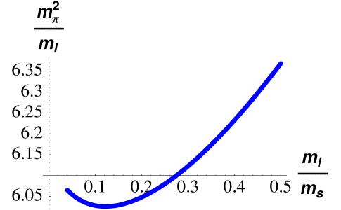
Figure 4: Typical behavior of $m_{\pi}^{2}/m_{l}$ as a function of $m_{l}/m_{s}$ at NLO.

Similar comments hold for $f_{K}/f_{\pi}$, plotted in fig. 5 using the same parameters except now $f=0.085\;$GeV (chosen so as to better match the experimental value at the lower end of the curve). Here the linear terms are larger, but an extrapolation accurate to a few percent still requires inclusion of the curvature.

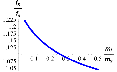
Figure 5: Typical behavior of $f_{K}/f_{\pi}$ as a function of $m_{l}/m_{s}$ at NLO.

(VII) The results further illustrate the utility of the lattice for obtaining LECs. In nature one can vary the valence content by considering different PGBs, while the sea content is fixed. Thus $L_{4}$ and $L_{6}$ are not accessible using the results above. On the lattice, however, one can change the sea quark masses and thus determine these LECs more easily. Using PQ simulations (varying valence and sea masses independently) further simplifies the determinations, as will be discussed in sec. 4.5.

2.4.2 Volume dependence from $\chi$PT

For single particle matrix elements, PGB loops loops give the leading correction due to the use of a finite spatial volume. To obtain the leading volume dependence, one simply replaces the momentum integrals with sums, e.g.

• 

  $\to\int_{q}\left(\frac{1}{q^{2}+m_{NG}^{2}}\right)\to\int_{q_{4}}\sum_{\vec{q}=2\pi\vec{n}/L}\left(\frac{1}{q^{2}+m_{NG}^{2}}\right)$ .

This is now done routinely when fitting lattice data. Figure 6 illustrates the rapid growth in finite volume shifts as the quark mass is reduced.

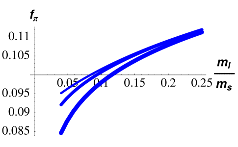
Figure 6: $f_{\pi}$ vs. $m_{l}/m_{s}$ at $a=0.1\;$fm, with $L=2.4\;$fm (thick), $3.2\;$fm (medium) and $\infty$ (thin), using $m_{s}=0.08\;$GeV, $f=0.08\;$GeV, $L_{5}=1.45\times 10^{-3}$, $L_{4}=0$.

Unfortunately, recent work suggests that an accurate estimate of volume corrections requires the inclusion of at least the dominant part of the two-loop contributions[34]. The requisite calculation has only been done for a few quantities, so for others one may be forced to work in volumes large enough that finite volume effects are negligible. For determining such volumes one-loop results should be a reliable guide if used conservatively.

If the quark mass is reduced at fixed box size satisfying $L\gg 1/\Lambda_{\rm QCD}$, one eventually enters the so-called “$\epsilon-$regime” where $m_{NG}L\mathrel{\hbox to0.0pt{\lower 3.0pt\hbox{$\mathchar 536\relax$}\hss}\raise 2.0pt\hbox{$\mathchar 316\relax$}}1$. Here the pion propagator is completely distorted by finite volume effects. It turns out, however, that one can still use $\chi$PT to predict the form of correlation functions[35]. I will not discuss this regime further, but note that there is an ongoing effort to determine the LECs of QCD (including electroweak interactions) by comparing the results of simulations in the $\epsilon-$regime to the predictions of $\chi$PT[36].

2.4.3 Convergence of $\chi$PT

I have only scratched the surface of calculations in $\chi$PT, which have been extended to include the electroweak Hamiltonian in the PGB sector and to NNLO (as reviewed, e.g., by Bijnens[37]). Many quantities are relevant for lattice simulations—I give a list below in sec. 4.5.1 when discussing PQ$\chi$PT. Here I only discuss what has been learned about the important question of convergence of $\chi$PT.

I quote one example[38], obtained from a fit of the $N=3$ NNLO formulae to a number of experimental inputs, but with the NNLO LECs estimated approximately using “single resonance saturation”. One of the input quantities is $f_{K}/f_{\pi}$, and this turns out to have a chiral expansion[37]

$$f_{K}/f_{\pi}=\underbrace{1}_{\textrm{LO}}+\underbrace{0.169}_{\textrm{NLO}}+\underbrace{0.051}_{\textrm{NNLO}}\,,$$ (35)

showing reasonable convergence. The convergence is less good, however, for the PGB masses.

The naive conclusion from this and similar results is that NNLO terms in $\chi$PT are needed for good accuracy. This is, I think, correct if one does a global fit to several quantities using $SU(3)$ $\chi$PT. One might, in practice, be able to get away with including only the analytic terms at NNLO (whose form is easy to determine) rather than the full two-loop expression. This is the approach used in the MILC analysis[3]. This amounts to mocking up the two-loop contributions by changing the NLO and NNLO LECs. While this makes the results for these LECs less reliable, I expect it to impact the extrapolated results for physical quantities only at the level of NNNLO corrections. Clearly, though, a full NNLO fit would be preferable.

Another approach which reduces the impact of NNLO terms is to use $SU(2)$ $\chi$PT alone, treating $m_{s}$ as heavy. After all, the actual extrapolation being done in present simulations is for the light quarks alone, with $m_{s}$ fixed near its physical value. In this approach the kaon and eta are treated as heavy particles, and one makes no assumption about the convergence of the expansion in $m_{s}$. The idea is that this removes the dominant contribution to the corrections in (35) and sums them to all orders. In practice, this approach has been used primarily in the baryon sector.

2.4.4 Extension to “heavy” particles

I will not describe $\chi$PT technology for including heavy particles here, but I do want to mention the form of the results. “Heavy” means $m_{\rm had}\mathrel{\hbox to0.0pt{\lower 3.0pt\hbox{$\mathchar 536\relax$}\hss}\raise 2.0pt\hbox{$\mathchar 318\relax$}}\Lambda_{\chi}$, and the approach is to expand in $1/m_{\rm had}$ so that at LO the hadron is a static source for PGBs. In this way one can include the dominant long-distance physics which gives rise to curvature at small light-quark mass.

The form of the resulting chiral expansion depends on the quantity considered. For heavy-light meson decay constants it is similar to that for PGB properties, e.g.

$$F_{B}\sim F_{B,0}(1+\underbrace{m_{\pi}^{2}}_{\textrm{analytic}}+\underbrace{m_{\pi}^{2}\ln(m_{\pi})}_{\textrm{ chiral log}}+\dots)$$ (36)

One new feature is that the non-analytic terms are not predicted in terms of the LO LECs, but involve an additional coefficient, $g_{\pi BB^{*}}$.

For baryons and vector meson masses the expansion differs further, involving odd powers of $m_{PGB}$.

$$M_{H}\sim M_{0}+\underbrace{m_{\pi}^{2}}_{\textrm{ analytic}}+\underbrace{g_{\pi HH^{\prime}}\ m_{\pi}^{3}}_{\textrm{ leading loop}}+\underbrace{m_{\pi}^{4}\ln(m_{\pi})}_{\textrm{ subleading loop}}+\ m_{\pi}^{4}+\dots$$ (37)

This means that the expansion is in powers of $m_{\pi}/\Lambda_{\chi}$ (c.f. $(m_{\pi}/\Lambda_{\chi})^{2}$ for PGBs and heavy-light mesons), so that the convergence is generically poorer. Thus it is even more important to use light quark masses when studying baryon properties.

3 Incorporating discretization errors into $\chi$PT

In this lecture I describe how for Wilson and twisted-mass fermions one can incorporate discretization errors into $\chi$PT, and what one learns by doing so. The method is general, and has been applied also to staggered fermions[8, 9], and to mixed-action theories[39]. See also the review by Bär[40].

3.1 Why incorporate discretization errors?

At first sight, it may seem strange to incorporate the effects of the ultraviolet (UV) cut-off of the underlying theory into the EFT describing its infrared (IR) behavior. The key point is that the UV effects break the chiral symmetry which determines the IR behavior. One way of saying this is that discretization errors lead to a non-trivial potential in the vacuum manifold which is otherwise flat due to the symmetry. As we will see, symmetry breaking due to quark masses and discretization errors have comparable effects on the potential if $m/\Lambda\approx(a\Lambda)^{2}$, with $\Lambda$ a scale of $O(\Lambda_{\rm QCD})$. The appropriate value of $\Lambda$ depends on the action, and it is quite possible that this condition is satisfied even for relatively fine lattices and light quarks. For example, if $\Lambda=500\;$MeV and $a^{-1}=2\;$GeV, then it is satisfied when $m=30\;$MeV. Thus it is imperative to study the impact of discretization errors.

One question that often arises in the present context is whether one should first extrapolate $a\to 0$ and then use continuum $\chi$PT, or do combined extrapolation in $a\to 0$ and $m\to m_{\rm phys}$. The possibilities are illustrated to the right.

An apparent advantage of the first approach is that one does not have to rely on the validity of $\chi$PT to do the continuum extrapolation; one simply uses a standard polynomial ansatz. There are, however, several reasons to use the second, “combined”, approach if $\chi$PT formulae are available:

• It incorporates relations between discretization errors in different quantities that follow from the specific way in which chiral symmetry is broken.

• It accounts for non-analyticities in $a$ which arise because of pion loops (e.g. for staggered fermions one has, schematically, $m_{\pi}^{2}\sim m_{q}[1+(m_{q}+a^{2})\ln(m_{q}+a^{2})+\dots]$). These might well be missed in a simple polynomial continuum extrapolation. The “$a^{2}$” in the chiral logs reduce the curvature, as clearly observed in the MILC results[3]. It should be kept in mind, however, that “$a^{2}$” always means “up to logs”, so not all non-analyticities are included.

• It accounts for changes in orientation of the condensate, which can be rapid with twisted-mass fermions if $m\sim a^{2}$, as discussed below.

3.2 General strategy

One proceeds in two steps[41]. First, following Symanzik[20], determine the continuum EFT describing the interactions of quarks and gluons with $|p|\ll 1/a$. Discretization errors enter with explicit factors of $a$, and are controlled by the symmetries (or lack thereof) of the underlying lattice theory. Second, use standard techniques to develop $\chi$PT for the Symanzik EFT. Since the latter is a continuum theory, this is no different conceptually from determining the effect of beyond-the-standard-model physics on the IR properties of QCD. The two steps are illustrated in Fig. 2 above.

3.3 Application to Wilson & twisted mass fermions

Twisted mass lattice QCD (tmLQCD)[42] has received a lot of recent attention because of its improved algorithmic properties and because, at maximal twist, physical quantities (including matrix elements) are automatically $O(a)$ improved[43]. Here it also serves as an excellent example, particularly as it contains Wilson fermions as a subset.

Twisting the mass in continuum QCD simply means doing an $SU(3)_{L}\times SU(3)_{R}$ rotation. The standard diagonal mass $M_{0}$ (which is hermitian assuming real $m_{q}$) is rotated into $M=U_{L}M_{0}U_{R}^{\dagger}$ which is not hermitian. The example I consider in detail has two degenerate flavors and

$$M=m_{q}e^{i\tau_{3}\omega}=m_{q}(\cos\omega+i\sin\omega\tau_{3})\equiv m+i\mu\tau_{3}\,,$$ (38)

resulting in a Lagrangian mass term containing a $\gamma_{5}\tau_{3}$ part:

$$\overline{Q}_{L}MQ_{R}+\overline{Q}_{R}M^{\dagger}Q_{L}=\overline{Q}(m+i\mu\gamma_{5}\tau_{3})Q\,.$$ (39)

Note that $m_{q}$ is the physical quark mass, with $m$ and $\mu$ respectively the untwisted and twisted components.

The “geometry” of the parameters is shown to the right. Although it naively appears that parity and flavor are broken, we know this is not the case since physics is unchanged by the chiral rotation. Thus $\omega$ is a redundant parameter. Usually, we keep the symmetries manifest by working at $\omega=0$, but it is important to know that we do not need to do so. The continuum

$\chi$PT analysis described above goes through for any $\omega$, as long as we expand about the rotated vacuum.

The situation is quite different after discretization. The lattice action is

$$S_{l,\rm glue}+a^{4}\sum_{x}\overline{\psi}_{l}D_{W}\psi_{l}+\overline{\psi}_{l,L}M\psi_{l,R}+\overline{\psi}_{l,R}M^{\dagger}\psi_{l,L}\,,$$ (40)

with $M$ the twisted mass, and the subscript “$l$” indicating “lattice”. Here $D_{W}$ is Wilson’s doubler-free derivative,

$${\rm D}\!\!\!\!/\,\longrightarrow D_{W}=\frac{1}{2}\sum_{\mu}\gamma_{\mu}(\nabla_{\mu}^{\ast}+\nabla_{\mu})-\frac{1}{2}\sum_{\mu}(\nabla_{\mu}^{\ast}\nabla_{\mu})$$ (41)

($\nabla$ and $\nabla^{\ast}$ are forward and backward derivatives, respectively). Since the second term in $D_{W}$ (the “Wilson term”, in which I have set the Wilson parameter $r=1$) breaks chiral symmetry, one cannot rotate away the twist in the mass. The theories with mass term $M_{0}$ and $U_{L}M_{0}U_{R}^{\dagger}$ are different on the lattice. In fact, the full fermion matrix $D_{W}+MP_{R}+M^{\dagger}P_{L}$ has positive determinant (and is thus useful in practice) only for special $M$. One such choice is two flavors with the twisted mass (38), for which the lattice action is

$${S}_{\rm tmLQCD}=S_{l,\rm glue}+a^{4}\sum_{x}\overline{\psi}_{l}\left(D_{W}+m_{0}+i\gamma_{5}\tau_{3}\mu_{0}\right)\psi_{l}\,.$$ (42)

Here $m_{0}$ and $\mu_{0}$ are, respectively, the bare untwisted and twisted mass (in lattice units). For the remainder of this lecture I will focus entirely on this theory.

3.4 Determining the local effective Lagrangian

Symanzik[20] showed how to study the approach of the lattice theory to its continuum limit. The first step is to understand this limit itself. The lattice provides a legitimate regularization of QCD (one that is awkward from a perturbative point of view, but has the great advantage of being non-perturbative), and so one obtains continuum QCD (in this case tmQCD) as the cut-off $1/a$ is sent to infinity. This has been established to all orders in perturbation theory[46] and it assumed to hold non-perturbatively. One must appropriately tune the (“relevant”) lattice bare parameters to reach the continuum limit. In particular, since the Wilson term mixes with the identity operator, $m_{0}$ is additively renormalized, and must be tuned to $m_{c}(a)<0$, while the twisted mass has nothing to mix with and is multiplicatively renormalized. The resulting continuum theory is

$$\mathcal{L}_{\rm tmQCD}=\mathcal{L}_{\rm glue}+\overline{\psi}({\rm D}\!\!\!\!/\,+m+i\gamma_{5}\tau_{3}\mu)\psi\,,$$ (43)

with $\mathcal{L}_{\rm glue}$ the usual continuum gluon action, and with the continuum field and physical masses being

$$\psi=a^{-3/2}Z\ \psi_{l}\,,\quad m=Z_{S}^{-1}(m_{0}-m_{c})/a\,,\quad{\rm and}\quad\mu=Z_{P}^{-1}\mu_{0}/a\,.$$ (44)

Here $Z$, $Z_{S}$ and $Z_{P}$ are renormalization factors relating quantities in the lattice regularization to those in the chosen continuum scheme. The corresponding geometry is illustrated below.

Corrections to the continuum limit are suppressed by inverse powers of the cut-off, i.e. by positive powers of $a$. Symanzik showed how these can collected into a local effective Lagrangian

$$\mathcal{L}_{\rm Sym}=\mathcal{L}_{\rm tmQCD}+a\mathcal{L}^{(5)}+a^{2}\mathcal{L}^{(6)}+\dots,$$ (45)

where $\mathcal{L}_{\rm tmQCD}$ is the desired continuum Lagrangian (note the absence of the “L” in the subscript), and $\mathcal{L}^{(5)}$ and $\mathcal{L}^{(6)}$ contain terms of dimension 5 and 6, respectively. The effective theory must be regularized, either by a standard continuum regulator such as dimensional regularization, or possibly with a finer lattice having $a^{\prime}\ll a$. We will not actually use $\mathcal{L}_{\rm Sym}$ for concrete calculations so do not need to be more specific. A key feature of $\mathcal{L}_{\rm Sym}$ is that all factors of $a$ are explicit—the effective theory does not “know” about the lattice spacing in any other way. Note, however, that “$a$” includes logarithms, of the form $\sim a[1+g(a)^{2}\ln a+\dots]$. I return to this point below.

The content of eq. (45) is that all discretization errors in all correlation functions can be reproduced by a set of local insertions. This is established by a procedure akin to renormalization (in which one determines divergent parts of graphs by doing a Taylor expansion in the external momenta, or a lattice variant of this procedure[46], and then subtracts them), except that one subtracts more terms in the Taylor expansion (“over-subtraction”), thus including those proportional to powers of $a$. As with renormalization, the consistency of this procedure requires that one include all terms in $\mathcal{L}^{(n)}$ of the appropriate dimension which are invariant under the symmetries of the theory—here, of tmLQCD. These terms will have coefficients such that reflection positivity is satisfied, since they arise from a theory in which it is satisfied. This procedure also works if one includes sources for external operators, which should be treated using the spurion trick. The procedure has been demonstrated to all orders in perturbation theory, and is assumed to work non-perturbatively.

The preceding discussion is nothing other than (a sketch of) a derivation of an EFT. The usual EFT words—“separation of scales”—were not mentioned but were implicit. $\mathcal{L}_{\rm Sym}$ is only useful if $p\ll 1/a$, for otherwise successive terms in the expansion, which give contributions of relative size $ap$, are not suppressed. Thus $\mathcal{L}_{\rm Sym}$ is an EFT for quarks and gluons with energies far below the cut-off scale. The set-up is the same as when considering the impact of new short-distance physics on QCD, except that the new physics here violates rotation and translation symmetries. It indicates how one can derive an EFT in a Euclidean context, at least order-by-order in perturbation theory. One does not need to rely on the S-matrix argument of Weinberg. This is important because the underlying lattice theory is discretized in Euclidean space.

Let me illustrate these general words with a simple example. Consider the quark-gluon vertex shown in Fig. 7. In EFT language, the counterterms $\mathcal{L}^{(5,6,\dots)}$ are to be determined by matching correlation functions with those of the lattice theory. At tree-level, the $O(a)$ terms in the lattice vertex can be matched by adjusting the coefficients of operators in $\mathcal{L}^{(5)}$ such as $\overline{\psi}D^{2}\psi$ as long as $|p|\ll 1/a$. At one-loop, for $|q|\ll 1/a$, the integrands match by construction, giving a logarithmic divergence. For larger $|q|$, however, the matching fails, leading to a finite difference in the results (finite since both theories are regulated). To match one must add an $O(g^{2})$ contribution to the coefficients of the operators in $\mathcal{L}^{(5)}$. One loop matching is schematically:

$$apg^{2}(\ln[pa]+r_{\rm lat}) = apg^{2}(\ln[pa^{\prime}]+r_{\rm EFT})+apg^{2}c^{(2)}_{\rm EFT}$$ (46)

$$\Rightarrow\quad c^{(2)}_{\rm EFT} = r_{\rm lat}-r_{\rm EFT}+\ln[a/a^{\prime}]\,,$$ (47)

where $r_{\rm lat,EFT}$ are the finite parts of the loop diagram, and I have used a lattice regularization of the EFT with spacing $a^{\prime}$. We can now see the generic form of the $a$ dependence of the coefficients in $\mathcal{L}^{(5)}$ (whose one-loop contribution is given here by $g^{2}c^{(2)}_{\rm EFT}$). There is explicit logarithmic dependence, and an implicit logarithmic dependence through $g$, which is evaluated in the lattice calculation at a scale $\sim a$.

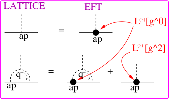
Figure 7: Matching lattice QCD with the Symanzik EFT. Dashed lines are gluons, solid lines quarks, $p\ll 1/a$ an external momentum, $q$ a loop momentum.

As an aside, I note that, having determined the form of $\mathcal{L}^{(5)}$ in the EFT, one can add corresponding terms to the lattice theory (i.e. terms having operators in $\mathcal{L}^{(5)}$ as their classical continuum limit), and then adjust the coefficients of the lattice terms to set those in $\mathcal{L}^{(5)}$ to zero. This is the “improvement program” at $O(a)$[20], and it has been implemented non-perturbatively[19, 47]. In the “new physics” context this would be called “fine tuning”, with negative connotations, but here we can again turn all the knobs at our disposal to improve extrapolations. The program can be extended, in principle, to any order, but has in practice not been extended to $\mathcal{L}^{(6)}$. Since $\mathcal{L}^{(6)}$ will play a key role in the following, this means that the considerations below are essentially unaffected by improvement.

3.5 Symanzik effective action for tmLQCD

We are now ready to determine the operators in $\mathcal{L}^{(5)}$ and $\mathcal{L}^{(6)}$. These must satisfy the symmetries of tmLQCD, eq. (42), and be reflection positive. The symmetries are gauge invariance, lattice rotations and translations, charge conjugation and fermion number, but not flavor $SU(2)$ nor parity (for generic $\omega$). Only the $U(1)$ flavor subgroup generated by $\tau_{3}$, and combinations of parity with a discrete flavor rotations survive:

$$\mathcal{P}^{1,2}_{F}:\quad\psi_{l}(x)\rightarrow\gamma_{0}(i\tau_{1,2})\psi_{l}(x_{P})\,,\ \ \overline{\psi_{l}}(x)\rightarrow\overline{\psi_{l}}(x_{P})(-i\tau_{1,2})\gamma_{0}\,,$$ (48)

Also useful is $\widetilde{\mathcal{P}}$: parity combined with $[\mu_{0}\rightarrow-\mu_{0}]$.

The continuum Lagrangian consistent with these symmetries is tmQCD, eq. (43). To determine $\mathcal{L}^{(5)}$ one simply enumerates all allowed operators, generalizing the work done for Wilson fermions[19]. The result is[48]

$$\mathcal{L}^{(5)} = b_{1}\overline{\psi}i\sigma_{\mu\nu}F_{\mu\nu}\psi+b_{2}\overline{\psi}({\rm D}\!\!\!\!/\,+m+i\gamma_{5}\tau_{3}\mu)^{2}\psi$$ (49)

$$+b_{3}m\overline{\psi}({\rm D}\!\!\!\!/\,+m+i\gamma_{5}\tau_{3}\mu)\psi+b_{4}m{L}_{\rm glue}+b_{5}m^{2}\overline{\psi}\psi$$

$$+b_{6}\mu\overline{\psi}\big{[}({\rm D}\!\!\!\!/\,+m+i\gamma_{5}\tau_{3}\mu),i\gamma_{5}\tau_{3}\big{]}_{+}\psi+b_{7}\mu^{2}\overline{\psi}\psi\,,$$

where I use continuum masses $m,\mu$ rather than bare masses. The coefficients $b_{i}$ (the analog of the LECs of $\chi$PT) are real (from reflection positivity), and depend on $g^{2}(a)$ and $\ln a$. Among them $b_{6,7}$ are “new” compared to Wilson case. Many terms have been forbidden by lattice symmetries: $\widetilde{P}$ forbids $m\mu\overline{\psi}\psi$ and $m^{2}\overline{\psi}i\gamma_{5}\tau_{3}\psi$, and it requires $\overline{\psi}\tau_{3}\gamma_{5}\psi$ to come with factor $\mu_{0}\propto\mu$, and the twisted Pauli term $\overline{\psi}\sigma_{\mu\nu}F_{\mu\nu}\tau_{3}\psi$ to have factor of $\mu$ (so that it appears in $\mathcal{L}^{(6)}$); flavor $U(1)$ forbids $\overline{\psi}\tau_{1,2}\psi$; and $\mathcal{P}^{1,2}_{F}$ forbids $\overline{\psi}\gamma_{5}\psi$, $\widetilde{F}_{\mu\nu}F_{\mu\nu}$ and $\overline{\psi}\tau_{3}\psi$.

$\mathcal{L}^{(5)}$ looks rather forbidding, with 7 unknown coefficients, but this proliferation is misleading, for two reasons. First, we will be doing a joint continuum-chiral expansion, and working in the “generic small mass” (GSM) regime in which $m\sim\mu\sim a\Lambda_{\rm QCD}^{2}$. Thus each factor of $m$ or $\mu$ counts as an additional power of $a$. We will work at NLO in this power counting. Since $\overline{\psi}{\rm D}\!\!\!\!/\,\psi$ and $\mathcal{L}_{\rm glue}$ map into LO operators in $\chi$PT, and $\mathcal{L}^{(5)}$ comes with an overall factor of $a$, any further factors of $m$ or $\mu$ make the operator of next-to-next-to-leading order (NNLO). This allows us to drop all except the $b_{1}$ term, and the $\overline{\psi}{\rm D}\!\!\!\!/\,^{2}\psi$ parts of the $b_{2}$ and $b_{3}$ terms. Second, we will be mapping $\mathcal{L}_{\rm Sym}$ into $\chi$PT, at which point all that matters is the chiral transformation properties of the operators. Now the Pauli ($b_{1}$) term and $\overline{\psi}{\rm D}\!\!\!\!/\,^{2}\psi$ transform the same way, so, since the coefficients in the mapping to $\chi$PT are unknown, we can drop the latter operator. The outcome is

$$\mathcal{L}_{\rm NLO}^{(5)}=b_{1}\overline{\psi}i\sigma_{\mu\nu}F_{\mu\nu}\psi\,,$$ (50)

which is unchanged from the result for (untwisted) Wilson fermions.

Moving onto $\mathcal{L}^{(6)}$, there are now gluonic terms[49]

$$\mathcal{L}_{\rm glue}^{(6)} \sim {\rm Tr}(D_{\mu}F_{\rho\sigma}D_{\mu}F_{\rho\sigma})+{\rm Tr}(D_{\mu}F_{\mu\sigma}D_{\rho}F_{\rho\sigma})$$ (51)

$$+\underbrace{{\rm Tr}(D_{\mu}F_{\mu\sigma}D_{\mu}F_{\mu\sigma})}_{\textrm{Lorentz violating}}+\underbrace{(m^{2},\mu^{2}){\rm Tr}(F_{\mu\nu}F_{\mu\nu})}_{\textrm{$O(a^{2}m^{2},a^{2}\mu^{2})$ so NNNLO}}\,,$$

where I use a schematic notation without coefficients, and fermionic terms (obtained by generalizing the analysis for Wilson fermions[50, 51])

$$\mathcal{L}_{q}^{(6)} \sim \underbrace{\overline{\psi}D_{\mu}^{3}\gamma_{\mu}\psi}_{\textrm{Euclidean non-invariant}}+\overline{\psi}D_{\mu}{\rm D}\!\!\!\!/\,D_{\mu}\gamma_{\mu}\psi+\dots$$ (52)

$$+\underbrace{m\overline{\psi}{\rm D}\!\!\!\!/\,^{2}\psi+\mu\overline{\psi}{\rm D}\!\!\!\!/\,^{2}i\gamma_{5}\tau_{3}\psi}_{\textrm{$O(a^{2}m,a^{2}\mu)$ so NNLO}}+\underbrace{m\overline{\psi}i\sigma_{\mu\nu}F_{\mu\nu}\psi+\mu\overline{\psi}\sigma_{\mu\nu}F_{\mu\nu}\gamma_{5}\tau_{3}\psi}_{\textrm{$O(a^{2}m,a^{2}\mu)$ so NNLO}}$$

$$+\underbrace{(m^{2},\mu^{2})\overline{\psi}{\rm D}\!\!\!\!/\,\psi+m\mu\overline{\psi}{\rm D}\!\!\!\!/\,i\gamma_{5}\tau_{3}\psi}_{\textrm{$O(a^{2}m^{2})$, etc. so NNNLO}}+\underbrace{(m^{3},m\mu^{2})\overline{\psi}\psi+(\mu^{3},\mu m^{2})i\gamma_{5}\tau_{3}\psi}_{\textrm{$O(a^{2}m^{3})$, etc. so NNNNLO}}$$

$$+(\overline{\psi}\psi)^{2}+(\overline{\psi}\gamma_{\mu}\psi)^{2}+\dots\,,$$

where the first ellipsis indicates other Euclidean invariant terms with three derivatives and the second other four-fermion operators. As can be seen, in the GSM regime, most of the fermionic operators in $\mathcal{L}^{(6)}$ are of at least NNLO. In particular, no flavor-parity breaking terms appear, since they require a factor a $\mu$. The net result is that the part of $\mathcal{L}^{(6)}$ of NLO in the GSM regime is the same as that for untwisted Wilson fermions (with the ellipses having the same meaning as above):

$$\mathcal{L}_{\rm NLO}^{(6)} \sim {\rm Tr}(D_{\mu}F_{\rho\sigma}D_{\mu}F_{\rho\sigma})+{\rm Tr}(D_{\mu}F_{\mu\sigma}D_{\rho}F_{\rho\sigma})$$ (53)

$$+\overline{\psi}D_{\mu}{\rm D}\!\!\!\!/\,D_{\mu}\gamma_{\mu}\psi+\dots+(\overline{\psi}\psi)^{2}+(\overline{\psi}\gamma_{\mu}\psi)^{2}+\dots$$

$$+\underbrace{{\rm Tr}(D_{\mu}F_{\mu\sigma}D_{\mu}F_{\mu\sigma})+\overline{\psi}D_{\mu}^{3}\gamma_{\mu}\psi}_{\textrm{Euclidean non-invariant}}\,.$$

Note that the only symmetry broken by $\mathcal{L}_{\rm NLO}^{(6)}$ that is not already broken by $\mathcal{L}_{\rm NLO}^{(5)}$ is Euclidean invariance. In fact, we will see that in the PGB sector the Euclidean non-invariant terms pick up an additional factor of $p^{2}$ and (given the overall $a^{2}$) are of NNLO.

This takes care of the action, but what about currents and densities? The matching of these between the lattice theory and the EFT can be worked out using symmetries[20], and I quote only the relevant results[19, 54]:

$$V_{\mu}^{b} = \overline{\psi}\gamma_{\mu}T^{b}\psi+a\tilde{c}_{V}\partial_{\nu}\overline{\psi}i\sigma_{\mu\nu}T^{b}\psi\,,$$ (54)

$$A_{\mu}^{b} = \overline{\psi}\gamma_{\mu}\gamma_{5}T^{b}\psi+a\tilde{c}_{A}\partial_{\mu}\overline{\psi}\gamma_{5}T^{b}\psi\,,$$ (55)

$$S^{0} = \overline{\psi}\psi+a\tilde{g}_{S}{\rm Tr}(F_{\mu\nu}F_{\mu\nu})\,,\qquad P^{b}=\overline{\psi}\gamma_{5}T^{b}\psi$$ (56)

Here I work at NLO in the GSM regime, so $am\sim a\mu$ terms are dropped. I also drop the mixing of $S^{0}$ with the identity operator, as it does not contribute to connected matrix elements. The coefficients $\tilde{c}_{V,A}$ and $\tilde{g}_{S}$ depend on $g(a)$ and on $\ln(a)$, just like the $b_{i}$ above. The content of these equations is that the on-shell matrix elements of the operators shown, evaluated in the EFT, will reproduce those of the lattice currents and densities, including the leading discretization error. These forms apply for any choice of lattice currents and densities (e.g. ultra-local or smeared) as long as they have been multiplied by appropriate $Z$-factors so as to be correctly normalized. The numerical values of the coefficients $\tilde{c}_{V}$ etc. will, of course, depend on the form of the lattice operators, and on the lattice action. In particular, if the action and operators have been $O(a)$ improved, then these coefficients will vanish. Note that the density $P^{b}$ is automatically improved.

When we map the operators in (54-56) into $\chi$PT we are free to do this for the $O(1)$ and $O(a)$ parts separately and then combine at the end. It is straightforward to see that the $\tilde{c}_{V}$ and $\tilde{g}_{S}$ terms map into operators which are of NNLO and can be dropped. For the former, the argument is given by Wu and I[55], and follows because of the need to have three derivatives in order to match the quark-level operator. For the $\tilde{g}_{S}$ term the argument is even more simple: the matching of chiral singlet ${\rm Tr}(F_{\mu\nu}F_{\mu\nu})$ gives the LO chiral kinetic term ${\rm Tr}(\partial_{\mu}\Sigma\partial_{\mu}\Sigma^{\dagger})$. Thus the $\tilde{g}_{S}$ term is of size $ap^{2}$, and so of NNLO compared to $\overline{\psi}\psi$, which maps to ${\rm Tr}(\Sigma+\Sigma^{\dagger})\sim O(1)$.

I conclude that, at NLO in the GSM regime, the currents and densities in the Symanzik EFT have the same form as in the continuum, aside from the $\tilde{c}_{A}$ term. Thus, as long as one treats the $\tilde{c}_{A}$ term separately, one can include the currents and densities using sources just as in continuum QCD, and the resulting theory will have a local chiral symmetry.

3.6 Mapping the Symanzik action into $\chi$PT

I now turn to the second step of the procedure—taking the Symanzik EFT and determining the chiral EFT which describes it at long distances. This was done for continuum Lagrangian, $\mathcal{L}_{\rm tmQCD}$, in sec. 2—a twisted mass was already included by the generality of the formalism. The result is $\mathcal{L}^{(2)}_{\chi}$ of eq. (28) at LO and $\mathcal{L}^{(4)}_{\chi}$ of eq. (31) at NLO. The task here is to include the effects of $\mathcal{L}^{(5,6)}$, as well as the $\tilde{c}_{A}$ term in eq. (55). To do so systematically requires a power counting scheme, to which I now turn.

3.6.1 Power counting and terminology

As anticipated above, discretization errors introduce a new parameter into the power counting in $\chi$PT. In addition to the usual chiral expansion in powers of $p^{2}/\Lambda_{\chi}^{2}\sim m_{NG}^{2}/\Lambda_{\chi}^{2}\sim m_{q}/\Lambda_{\rm QCD}$, we must include $a\Lambda_{\rm QCD}$. Note that $\Lambda_{\rm QCD}$ is the only scale available to balance dimensions when we map quark-level operators in $\mathcal{L}_{\rm Sym}$ into $\chi$PT. I stress that, once one has the Symanzik EFT in hand, $m$ and $a$ are on a similar footing—both are simply small parameters in a continuum Lagrangian.

How we should weight discretization errors relative to mass corrections? The numerical comparison is shown in Fig. 8. I have been conservative by having “present simulations” range down to $m_{s}/10$, which is yet to be achieved with Wilson-like fermions. I conclude from the figure that the appropriate power counting for the coming decade is $a^{2}\Lambda_{\rm QCD}^{3}\mathrel{\hbox to0.0pt{\lower 3.0pt\hbox{$\mathchar 536\relax$}\hss}\raise 2.0pt\hbox{$\mathchar 316\relax$}}m_{q}\mathrel{\hbox to0.0pt{\lower 3.0pt\hbox{$\mathchar 536\relax$}\hss}\raise 2.0pt\hbox{$\mathchar 316\relax$}}a\Lambda_{\rm QCD}^{2}$, and that to disentangle quark mass dependence from discretization effects we need to remove errors of $O(a)$ and understand those of $O(a^{2})$.

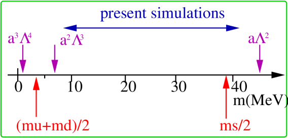
Figure 8: Comparing discretization errors to mass corrections. I use $a^{-1}=2\;$GeV and $\Lambda=300\;$MeV.

I will consider in the following two regimes (sketched below):

I. The GSM regime, already introduced above, which I define more precisely as $a\Lambda_{\rm QCD}^{2}\mathrel{\hbox to0.0pt{\lower 3.0pt\hbox{$\mathchar 536\relax$}\hss}\raise 2.0pt\hbox{$\mathchar 316\relax$}}m_{q}\ll\Lambda_{\rm QCD}$, so that it includes $a\Lambda_{\rm QCD}^{2}\ll m_{q}$ (where we would like to be) as well as $a\Lambda_{\rm QCD}^{2}\approx m_{q}$ (where we actually are). This is the regime in which we want to learn how to remove $O(a)$ errors.

II. The “Aoki regime”, in which $m_{q}\mathrel{\hbox to0.0pt{\lower 3.0pt\hbox{$\mathchar 536\relax$}\hss}\raise 2.0pt\hbox{$\mathchar 316\relax$}}a^{2}\Lambda_{\rm QCD}^{3}\ll\Lambda_{\rm QCD}$ (including $m_{q}\ll a^{2}\Lambda_{\rm QCD}^{3}$). This is where we cannot avoid discretization errors, and where they lead to non-trivial phase structure. Entering this regime changes the relative weight given to operators in $\chi$PT, but not the operators themselves.

I begin by working in the GSM regime at NLO. This requires keeping terms of $O(a^{2})$, and thus up to $\mathcal{L}^{(6)}$ in the Symanzik expansion. The enumeration will turn out to suffice also for a LO study of the Aoki regime.

3.6.2 Mapping $\mathcal{L}_{\rm NLO}^{(5)}$ and $\mathcal{L}_{\rm NLO}^{(6)}$ into $\chi$PT

$\mathcal{L}_{\rm NLO}^{(5)}$ transforms just like a mass term under $SU(2)_{L}\times SU(2)_{R}$ (recall that we set $N=2$, although the considerations are easily generalized):

$$a\mathcal{L}_{\rm NLO}^{(5)}\sim a\overline{\psi}i\sigma_{\mu\nu}F_{\mu\nu}\psi=\overline{\psi}_{L}\widetilde{A}i\sigma_{\mu\nu}F_{\mu\nu}\psi_{R}+\overline{\psi}_{R}\widetilde{A}^{\dagger}i\sigma_{\mu\nu}F_{\mu\nu}\psi_{A}\,.$$ (57)

Here $\widetilde{A}$ is a spurion transforming like $M$, i.e. $\widetilde{A}\to U_{L}\widetilde{A}U_{R}^{\dagger}$, so that $\mathcal{L}_{\rm NLO}^{(5)}$ is invariant. At the end we set $\widetilde{A}=a$. The enumeration of operators in the chiral Lagrangian is like that for $M$, yielding the new terms[52, 51, 53, 55]

$$\mathcal{L}^{(2)}_{\chi,A}=-\frac{{f}^{2}}{4}{\rm tr}(\hat{A}^{\dagger}\Sigma+\Sigma^{\dagger}\hat{A})$$ (58)

$$\mathcal{L}^{(4)}_{\chi,A}={W_{45}}{\rm tr}(D_{\mu}\Sigma^{\dagger}D_{\mu}\Sigma){\rm tr}(\hat{A}^{\dagger}\Sigma+\Sigma^{\dagger}\hat{A})-{W_{68}^{\prime}}\big{[}{\rm tr}(\hat{A}^{\dagger}\Sigma+\Sigma^{\dagger}\hat{A})\big{]}^{2}$$ (59)

$$-{W_{68}}{\rm tr}(\chi^{\dagger}\Sigma+\Sigma^{\dagger}\chi){\rm tr}(\hat{A}^{\dagger}\Sigma+\Sigma^{\dagger}\hat{A})+{W_{10}}{\rm tr}(D_{\mu}\hat{A}^{\dagger}D_{\mu}\Sigma+D_{\mu}\Sigma^{\dagger}D_{\mu}\hat{A})$$

$$-{H^{\prime}_{2}}{\rm tr}(\hat{A}^{\dagger}\chi+\chi^{\dagger}\hat{A})-{H_{3}}{\rm tr}(\hat{A}^{\dagger}\hat{A})\,,$$

where $\hat{A}=2{W_{0}}\widetilde{A}$ is the analog of $\chi=2{B_{0}}(s+ip)$, with $W_{0}$ a new LEC at LO. We will not need to use $\hat{A}$ as a source (since we already have $\chi$), so we will always be set $\hat{A}\to\hat{a}=2W_{0}a$. $SU(2)$ simplifications can then reduce the number of terms. In particular $(\hat{A}^{\dagger}\Sigma+\Sigma^{\dagger}\hat{A})$ is proportional to the identity, allowing single trace terms involving this combination to be rewritten with two traces. These simplifications have been used in (59).

Note that, following the discussion at the end of sec. 3.5, I have included sources for currents and densities and enforced local chiral invariance by using covariant derivatives $D_{\mu}$ [defined as in eq. (27)]. This incorporates all discretization effects in lattice matrix elements except those due to the $\tilde{c}_{A}$ term in eq. (55), which I will treat separately below.

${\mathcal{L}}_{\rm NLO}^{(6)}$ contains three types of terms. First, those that are invariant under Euclidean and chiral symmetries [the gluonic terms on the first line of eq. (53) and some of the four-fermion operators]. These match into $\chi$PT as follows:[8]

$$a^{2}{\rm Tr}(D_{\mu}F_{\rho\sigma}D_{\mu}F_{\rho\sigma})+\dots+a^{2}\overline{\psi}D_{\mu}{\rm D}\!\!\!\!/\,D_{\mu}\gamma_{\mu}\psi+\dots\longrightarrow a^{2}{\rm tr}(D_{\mu}\Sigma D_{\mu}\Sigma^{\dagger})\,,$$ (60)

i.e. one obtains the leading order continuum result multiplied by $a^{2}$. This leads to an $O(a^{2})$ correction to the LEC $f$, and is present for any fermion discretization (including chirally invariant ones).

Second, there are four-fermion operators which violate chiral symmetry (e.g. those having LR-LR structure). Their matching can be analyzed using two $\hat{A}$ spurions, leading to[51]

$$(\overline{\psi}\psi)^{2}+(\overline{\psi}\gamma_{\mu}\psi)^{2}+\dots\longrightarrow{\rm tr}\left[(\hat{A}^{\dagger}\Sigma+\Sigma^{\dagger}\hat{A})\right]^{2}\,.$$ (61)

This operator is already present in $\mathcal{L}^{(4)}_{\chi,A}$, having been produced by two insertions of $\mathcal{L}^{(5)}_{NLO}$. This illustrates that what is relevant for matching are the symmetries broken by the operators (here, chiral symmetry), and not their detailed form. The four-fermion operators simply change an unknown coefficient, $W^{\prime}_{68}$, by an unknown amount. The only exception is if one uses a non-perturbatively $O(a)$ improved quark action, as discussed below, when $W^{\prime}_{68}$ would vanish were it not for the four-fermion operators.

Finally, there are the terms violating Euclidean symmetry. These can be decomposed into Euclidean singlet and non-singlet parts. The former match as in eq. (60), while the latter give rise to Euclidean non-invariant chiral operators[8]

$$a^{2}{\rm Tr}(D_{\mu}F_{\mu\sigma}D_{\mu}F_{\mu\sigma})+a^{2}\overline{\psi}D_{\mu}^{3}\gamma_{\mu}\psi\longrightarrow a^{2}{\rm tr}(D_{\mu}^{2}\Sigma D_{\mu}^{2}\Sigma^{\dagger})\,.$$ (62)

Since one needs four factors of $D_{\mu}$ to make a non-invariant operator, the result, when combined with the two powers of $a$, is an operator of NNNLO in $\chi$PT, two orders higher than we are working.

We thus find that ${\mathcal{L}}_{\rm NLO}^{(6)}$ adds no new operators, so the results (58) and (59) are complete. They are to be added to $\mathcal{L}^{(2)}_{\chi}$ [eq. (28)] and $\mathcal{L}^{(4)}_{\chi}$ [eq. (31)], respectively, to obtain the full LO and NLO contributions to the chiral Lagrangian in the GSM regime. Note that using a twisted mass had no impact on the analysis of this subsection, since $\mathcal{L}_{\rm NLO}^{(5,6)}$ have the same form as for untwisted Wilson fermions.

I now return to the $\tilde{c}_{A}$ term in the axial current, eq. (55). To obtain the full axial current in the EFT one must separately match this term into $\chi$PT and add it to the result obtained by taking derivatives of the Lagrangian obtained above with respect to sources. It is a simple exercise to show, however, that the result is simply to change the coefficient $W_{10}$, since the operator it multiplies is exactly of the form $a\partial_{\mu}P^{b}$, at linear order in the sources. Thus the final form of the previous paragraph remains complete, albeit with somewhat changed (although still unknown) coefficients.

There are thus five new LECs introduced by discretization errors: $W_{0}$ at LO, $W_{45}$, $W_{68}$, $W^{\prime}_{68}$ and $W_{10}$ at NLO. What do we know about their values? Of course this depends on the choice of fermion and gauge actions, so we can only make order of magnitude estimates. Perturbing in $a$ and $m$ after rotating to Minkowski space, one finds

$$\frac{W_{0}}{B_{0}}\sim\frac{\langle\pi|\overline{\psi}i\sigma_{\mu\nu}F^{\mu\nu}\psi|\pi\rangle}{\langle\pi|\overline{\psi}\psi|\pi\rangle}\sim\Lambda_{\rm QCD}^{2}\,.$$ (63)

The first relation is not an equality because there are unknown coefficients multiplying numerator and denominator, while the second is a dimensional estimate. One might be tempted to include a loop factor because the matrix element in the numerator requires at least one gluon loop, but this is a non-perturbative matrix element so such counting is inappropriate.

The four NLO $W_{i}$ are dimensionless, because the dimensions needed to balance powers of $a$ are provided by the $W_{0}$ residing in $\hat{A}$. Like the Gasser-Leutwyler coefficients $L_{i}$, they depend on the renormalization scale, $\mu$. We will find that the combinations

$$\widetilde{W}=W_{45}-L_{45}\,,\quad W=W_{68}-2L_{68}\,,\ \textrm{and}\ W^{\prime}=W^{\prime}_{68}-W_{68}+L_{68}$$ (64)

are $\mu$ independent, so the scale dependence of the $W_{i}$ themselves is comparable to that of the $L_{i}$. Using the argument of sec. 2.3.5, we then estimate $|W_{i}|\sim|L_{i}|\sim 1/(4\pi)^{2}$. Another line of argument gives a similar estimate. In continuum $\chi$PT, $\overline{\psi}\psi$ maps into $\mathcal{O}=f^{2}2B_{0}{\rm tr}(\Sigma+\Sigma^{\dagger})/4$. Thus we expect the mapping of $a^{2}(\overline{\psi}\psi)^{2}$ to contain $O(1)\times a^{2}\mathcal{O}^{2}$ plus other operators. In fact, this four-fermion operator (along with others) maps into $a^{2}\mathcal{O}^{2}16W^{\prime}_{68}W_{0}^{2}/(f^{4}B_{0}^{2})$. Comparing, and using eq. (63), I find $W^{\prime}_{68}\sim(1/16)(f/\Lambda_{\rm QCD})^{4}$. It is reassuring that this estimate, albeit crude, agrees with the order of magnitude of that above.

The analysis to this point has assumed that the fermion action is not non-perturbatively improved. Since many simulations now use such improvement, it is interesting to ask how it changes the analysis. Improvement sets $\mathcal{L}^{(5)}_{NLO}$ to zero. Since this was the source of almost all terms linear in $a$ in $\mathcal{L}^{(2,4)}_{\chi,A}$ above, the impact is to set $\mathcal{L}^{(2)}_{\chi,A}=W_{45}=W_{68}=0$. The term quadratic in $a$, with coefficient $W^{\prime}_{68}$ survives, since this also comes from matching with $\mathcal{L}^{(6)}_{NLO}$. Two coefficients of terms linear in $a$ do not vanish: $W_{10}$ and $H^{\prime}_{3}$. Why? As already noted, the former multiplies a term which only contributes if the source for the axial current is non-vanishing (the part containing the vector current cancels). It thus represents discretization errors in the matrix elements of this current. But these matrix elements require improvement additional to that of the action, namely the addition of the “$c_{A}$ term” to the axial current[19]. If this improvement has not been implemented, then $W_{10}\neq 0$. Note that, following the discussion at the end of sec. 3.5, the matrix elements of the vector current and the densities are automatically improved (at NLO) if the action is improved.

The non-vanishing of $H^{\prime}_{3}$ even with non-perturbative improvement is a consequence of the improvement being on-shell. Contact terms in correlation functions are not improved, and this translates into the HECs of $O(a)$ being non-zero. This is, however, an academic point, since the only quantity of interest affected by $H^{\prime}_{3}$ is the scalar condensate[55], and this is very difficult to calculate in practice on the lattice.

3.7 Results for $m_{q}\sim a\Lambda_{\rm QCD}^{2}$ (GSM regime)

We are now ready to reap the benefits of the work we have done setting up $\chi$PT for tmLQCD, which I will call tm$\chi$PT. We can already see one benefit of the $\chi$PT technology: although there are several unknown LECs describing discretization errors, no more are needed for the entire twisted mass plane than for the untwisted Wilson mass axis.

In this section I discuss the results in the GSM regime, first at LO and then at NLO.

3.7.1 Tm$\chi$PT at LO

The complete LO Lagrangian include discretization errors is

$$\mathcal{L}^{(2)}_{\chi,{\rm GSM}} = \frac{{f}^{2}}{4}{\rm tr}(D_{\mu}\Sigma D_{\mu}\Sigma^{\dagger})-\frac{{f}^{2}}{4}{\rm tr}(\chi^{\dagger}\Sigma+\Sigma^{\dagger}\chi)-{\frac{{f}^{2}}{4}{\rm tr}(\hat{A}^{\dagger}\Sigma+\Sigma^{\dagger}\hat{A})}\,.$$ (65)

It will be useful to change the notation for sources:

$$\chi=2B_{0}(s+ip)=2B_{0}(m+i\mu\tau_{3})+\delta\chi\,,\qquad\delta\chi=2B_{0}(\delta s+i\delta p)\,.$$ (66)

We now make the simple but important observation that the factors of $\hat{A}$ can be absorbed by using the shifted variable[41] $\chi^{\prime}=\chi+\hat{A}$:

$$\mathcal{L}^{(2)}_{\chi,{\rm GSM}} = \frac{{f}^{2}}{4}{\rm tr}(D_{\mu}\Sigma D_{\mu}\Sigma^{\dagger})-\frac{{f}^{2}}{4}{\rm tr}(\chi^{\prime\dagger}\Sigma+\Sigma^{\dagger}\chi^{\prime})\,.$$ (67)

The result has exactly the same form as the LO continuum Lagrangian. The shift $\chi\to\chi^{\prime}$ corresponds to an $O(a)$ shift in the untwisted mass, $m\to m^{\prime}=m+a{W_{0}}/{B_{0}}$, but leaves $\delta s$ (and, indeed, $\delta\chi$) unchanged.. Recalling the definition of $m$, eq. (44), this is equivalent to a shift in the critical mass, $\Delta m_{c}=-a^{2}{Z_{S}W_{0}}/{B_{0}}$. This shift is not measurable, however, since $m_{c}$ is not known a priori. It must be determined non-perturbatively from the simulation itself. The traditional definition is that $m_{c}$ is the bare mass at which $m_{\pi}^{2}\to 0$ on the Wilson axis. Since at LO $\mathcal{L}^{(2)}_{\chi,{\rm GSM}}$ predicts $m_{\pi}^{2}\propto m^{\prime}$, we discover that this “$m_{\pi}^{2}$” definition of $m_{c}$ automatically includes the $O(a^{2})$ shift in $m_{c}$, and chooses the untwisted quark mass to be $m^{\prime}$.

The upshot is that, with the standard numerical definition of $m_{c}$, the pion and vacuum sectors are automatically $O(a)$ improved at LO in tm$\chi$PT for any twist angle. The analysis of this theory is as in the continuum and I sketch it quickly. The twist angle $\omega_{0}$ is defined by

$$(m^{\prime}+i\tau_{3}\mu)\equiv m_{q}e^{i\omega_{0}\tau_{3}}\,,\quad(m_{q}\ \textrm{real and positive})$$ (68)

giving the geometry shown below (note the renormalized axes).

The potential is minimized when $\Sigma$ is aligned with $\chi^{\prime}$: $\langle\Sigma\rangle=\exp(i\omega_{0}\tau_{3})$. It is conventional to expand $\Sigma$ about the condensate in a symmetric way,

$$\Sigma=\xi_{0}\;\Sigma_{ph}\;\xi_{0}\,,\quad\xi_{0}\equiv exp(i\omega_{0}\tau_{3}/2)\,,\quad\Sigma_{ph}\equiv\exp(i\vec{\pi}\cdot\vec{\tau}/f)\,,$$ (69)

since this corresponds diagonalizing the mass matrix with an axial transformation. The resulting theory is

$$\mathcal{L}_{\chi,\rm LO} = \frac{{f}^{2}}{4}{\rm tr}(D_{\mu}\Sigma_{ph}D_{\mu}\Sigma_{ph}^{\dagger})-\frac{{f}^{2}}{4}{\rm tr}\left\{\left[\widehat{m_{q}}+(\delta\chi)_{ph}^{\dagger}\right]\Sigma_{ph}+\textrm{h.c.}\right\}\,,$$ (70)

where $\widehat{m_{q}}\equiv 2B_{0}m_{q}$ and “h.c.” is hermitian conjugate. The masses and interactions of the pions are manifestly independent of $\omega_{0}$, since the mass term has been “untwisted”. At the same time, however, sources have been twisted: $(\delta\chi)_{ph}^{\dagger}=\xi_{0}(\delta\chi)^{\dagger}\xi_{0}$ and

$$D_{\mu}\Sigma_{ph}=\partial_{\mu}\Sigma_{ph}-il_{\mu}^{ph}\Sigma_{ph}+i\Sigma_{ph}r_{\mu}^{ph}\,,\ \textrm{with}\ l_{\mu}^{ph}=\xi_{0}^{\dagger}l_{\mu}\xi_{0}\,,\ r_{\mu}^{ph}=\xi_{0}r_{\mu}\xi_{0}^{\dagger}\,.$$ (71)

The operators used to determine physical matrix elements (obtained by functional derivatives with respect to the physical sources) are thus related to those in the lattice theory (obtained using the original sources) by an $\omega_{0}$-dependent twist. This reproduces the twisting one finds at the quark level: fields in the original (or “twisted”) basis [that with $M=m_{q}\exp(i\omega_{0}\tau_{3})$] are related to those in the “physical basis” [$M=m_{q}$] by an axial transformation [$\psi_{ph}=\exp(i\omega_{0}\tau_{3}\gamma_{5}/2)\psi$], so that operators are also transformed[42], e.g.

$$\overline{u}_{ph}\gamma_{\mu}\gamma_{5}d_{ph}=\cos\omega_{0}(\overline{u}\gamma_{\mu}\gamma_{5}d)-i\sin\omega_{0}(\overline{u}\gamma_{\mu}d)\,.$$ (72)

Thus, at maximal twist ($\omega_{0}=\pi/2$) the charged pion should be created with the lattice vector current.

3.7.2 tm$\chi$PT at NLO

The NLO Lagrangian, rewritten in terms of $\chi^{\prime}$, and dropping HECs, is

$$\mathcal{L}^{(4)}_{\chi,{\rm GSM}}=\mathcal{L}^{(4)}_{\chi}+\mathcal{L}^{(4)}_{\chi,A}$$ (73)

$$=-{L_{13}}{\rm tr}(D_{\mu}\Sigma D_{\mu}\Sigma^{\dagger})^{2}-L_{2}{\rm tr}(D_{\mu}\Sigma D_{\nu}\Sigma^{\dagger}){\rm tr}(D_{\mu}\Sigma D_{\nu}\Sigma^{\dagger})$$

$$+{L_{45}}{\rm tr}(D_{\mu}\Sigma^{\dagger}D_{\mu}\Sigma){\rm tr}(\chi^{\prime\dagger}\Sigma+\Sigma^{\dagger}\chi^{\prime})-{L_{68}}\big{[}{\rm tr}(\chi^{\prime\dagger}\Sigma+\Sigma^{\dagger}\chi^{\prime})\big{]}^{2}$$

$${+{\widetilde{W}}{\rm tr}(D_{\mu}\Sigma^{\dagger}D_{\mu}\Sigma){\rm tr}(\hat{A}^{\dagger}\Sigma+\Sigma^{\dagger}\hat{A})-{W}{\rm tr}(\chi^{\prime\dagger}\Sigma+\Sigma^{\dagger}\chi^{\prime}){\rm tr}(\hat{A}^{\dagger}\Sigma+\Sigma^{\dagger}\hat{A})}$$

$${-{W^{\prime}}\big{[}{\rm tr}(\hat{A}^{\dagger}\Sigma+\Sigma^{\dagger}\hat{A})\big{]}^{2}+{W_{10}}{\rm tr}(D_{\mu}\hat{A}^{\dagger}D_{\mu}\Sigma+D_{\mu}\Sigma^{\dagger}D_{\mu}\hat{A})}\,.$$

Here I used $SU(2)$ relations to combine terms, eq. (31), with $L_{13}=L_{1}+L_{3}/2$, $L_{45}=L_{4}+L_{5}/2$ and $L_{68}=L_{6}+L_{8}/2$. I have also used the shifted $W$’s defined in eq. (64). The latter, as noted above, turn out to be independent of the renormalization scale. If we are using a non-perturbatively $O(a)$ improved action then $W=\widetilde{W}=0$, and if we also improve the axial current then $W_{10}=0$.

Subsequent results are simplified by the observation that $W_{10}$ is redundant[55]. A change of variables, $\delta\Sigma=({2}{W_{10}}/{f^{2}})\left(\Sigma\hat{A}^{\dagger}\Sigma-\hat{A}\right)$, which keeps $\Sigma\in SU(3)$ up to NNLO corrections, cancels the $W_{10}$ term while shifting the other LECs: $W\to W+W_{10}/4$ and $\widetilde{W}\to\widetilde{W}+W_{10}/2$. Because of this, I set $W_{10}=0$ henceforth. Note that if one uses a non-perturbatively $O(a)$ improved action but an unimproved axial current, then after this change of variables $W$ and $\widetilde{W}$ no longer vanish, but are related by $2W-\widetilde{W}=0$.

I now present a sampling of NLO results[53, 58, 55, 56]. These require as a first step the determination of the condensate about which to expand, and this is realigned by NLO terms. In the continuum there is no realignment, because the $L_{68}$ term is already extremized by the LO condensate, $\langle\Sigma\rangle=\exp(i\omega_{0}\tau_{3})\propto\chi^{\prime}$. The “discretization terms” (those proportional to $W$ and $W^{\prime}$) do, however, lead to a realignment, because they “pull” the condensate either towards or away from the identity direction. The result is:

$$\langle\Sigma\rangle=e^{i(\omega_{0}+\epsilon)\tau_{3}}\,,\quad\epsilon=-\frac{16\hat{a}\sin\omega_{0}}{f^{2}}\left({W}+2{W^{\prime}}\cos\omega_{0}\frac{\hat{a}}{\widehat{m_{q}}}\right)$$ (74)

Note that $\epsilon$ vanishes on the Wilson axis ($\omega_{0}=0,\pi$), and that the $W^{\prime}$ contribution is enhanced if $\widehat{m_{q}}\ll\hat{a}$ (in which case one enters the Aoki regime, where an $O(1)$ vacuum realignment is possible, as discussed below).

While $\epsilon$ is not measurable in simulations (as it is defined within $\chi$PT and not in terms of observables), it illustrates the typical magnitude of NLO effects. Given that we expect $|W|,|\widetilde{W}|,|W^{\prime}|\sim 1/(4\pi)^{2}$ and $W_{0}\sim\Lambda_{\rm QCD}^{3}$, it follows that $\epsilon\sim a\Lambda_{\rm QCD}$. To implement these expectations, it is useful to use rescaled variables[59]

$${\delta_{W}}=\frac{16\hat{a}W}{f^{2}}\sim a\Lambda_{\rm QCD},\ {\delta_{\widetilde{W}}}=\frac{16\hat{a}\widetilde{W}}{f^{2}}\sim a\Lambda_{\rm QCD},\ w^{\prime}=\frac{16\hat{a}^{2}W^{\prime}}{f^{2}}\sim a^{2}\Lambda_{\rm QCD}^{4}.$$ (75)

The general form of NLO results for observables is illustrated by

$$m_{\pi^{\pm}}^{2} = \widehat{m_{q}}\left[1+\frac{1}{2}L_{\pi}+\frac{16}{f^{2}}\widehat{m_{q}}(2L_{68}-L_{45})\right]$$ (76)

$$+\widehat{m_{q}}\cos\omega_{0}{(2\delta_{W}-\delta_{\widetilde{W}})}+2(\cos\omega_{0})^{2}w^{\prime}\,.$$

The first line is the continuum NLO result [the $SU(2)$ version of eq. (32), with chiral logs defined in (33)], while the second shows the impact of discretization. Recall that $\widehat{m_{q}}$ is defined to be positive. The scale dependence of the chiral log is absorbed by $2L_{68}-L_{45}$, leaving $2\delta_{W}-\delta_{\widetilde{W}}$ scale invariant. Chiral logs do not contain discretization corrections at this order because the LO discretization errors can be absorbed into $\chi^{\prime}$.

The result (76) shows the different possibilities for removing $O(a)$ errors.

• Non-perturbatively $O(a)$ improve the quark action, in which case $2\delta_{W}-\delta_{\widetilde{W}}=0$ and the $O(a)$ term vanishes.

• Use “mass averaging”[43] in which one averages over $\omega_{0}$ and $\omega_{0}+\pi$ at fixed $\widehat{m_{q}}$. This flips the sign of both $m^{\prime}$ and $\mu$, and thus of $\cos\omega_{0}$, and cancels the $O(a)$ term. It has been shown to lead to $O(a)$ improvement for all physical quantities, including matrix elements[43].

• Work at maximal twist, $\omega=\pm\pi/2$ (both choices of sign are equivalent, and I use the positive sign henceforth). This removes the $O(a)$ term (as it must since it is a special case of mass averaging where the average is automatic[43]), and, in this case though not in general, also the $O(a^{2})$ term.

I note two further features of the result (76). The $O(a)$ errors are determined throughout the twisted-mass plane by the combination $2\delta_{W}-\delta_{\widetilde{W}}$. In particular, on the Wilson axis, this term predicts an asymmetry in the slopes on the two sides of $m_{c}$. This has recently been observed numerically, as part of the initial studies of the properties of tmLQCD. I show an example of the results in Fig. 9. Defining the asymmetry in a quantity $Q$ as[59]

$${\rm AS}(Q)\equiv\frac{Q(m^{\prime},\mu)-(-)^{p}Q(-m^{\prime},\mu)}{Q(m^{\prime},\mu)+(-)^{p}Q(-m^{\prime},\mu)}\,,$$ (77)

(with $p$ a parity which is +1 for most quantities), one finds

$${\rm AS}(m_{\pi^{\pm}}^{2})=({m^{\prime}}/{m_{q}}){(2\delta_{W}\!-\!\delta_{\widetilde{W}})}\stackrel{{\scriptstyle\mu=0}}{{\longrightarrow}}{(2\delta_{W}-\delta_{\widetilde{W}})}\,.$$ (78)

The observed asymmetry in fig. 9 is $\sim 0.3$, consistent with the expected size ($a^{-1}\approx 1\;$GeV and $\Lambda_{\rm QCD}\approx 0.3\;$GeV).

Figure 9: Unquenched results for $(am_{\pi})^{2}$ as a function of $(2\kappa)^{-1}=m_{0}+4$ for $\mu=0$ and with $a^{-1}\approx 0.2\;$fm[60]. Straight lines are to guide the eye.

The second feature of (76) that I want to emphasize is that the $w^{\prime}$ term (proportional to $a^{2}$) gives an additive correction to $m_{\pi}^{2}$. This is indicative of the breaking of chiral symmetry. It can be of either sign. If $w^{\prime}>0$ then one expects a minimum pion mass, as observed in fig. 9, while if $w^{\prime}<0$ the pion mass-squared can become negative, indicating an instability. This leads to the well-known Aoki phase[61].

A graphic demonstration of the impact of discretization errors is provided by the contours of $m_{\pi}^{2}$ in the twisted mass plane. Examples are shown later in fig. 14. At LO the contours are circles (as in the continuum), indicating that $\omega_{0}$ is redundant, but they are significantly deformed by the discretization errors that enter at NLO.

Discretization errors linear in $a$ can be separated from the continuum parts of the predictions by using the asymmetries defined above. These are pure discretization effects, while the corresponding symmetries are $O(a)$ improved because symmetrization is the essentially the same as mass averaging. The asymmetries for quantities accessible with simulations are[55, 59]

$$\!\!\!\!\!\!\!\!2\,{\rm AS}(\langle 0|P^{\mp}|\pi^{\pm}\rangle) = AS(\langle\pi|S^{0}|\pi\rangle)={\rm AS}(m_{\pi^{\pm}}^{2})=({m^{\prime}}/{m_{q}}){(2\delta_{W}\!-\!\delta_{\widetilde{W}})}$$ (79)

$${\rm AS}(f_{\pi}) = (m^{\prime}/m_{q}){\delta_{\widetilde{W}}}/2\,,\qquad{\rm AS}(m_{\rm PCAC})=({m_{q}}/{m^{\prime}}){\delta_{W}}\,.$$ (80)

What is predicted here are the form of the mass dependence, and the relations between asymmetries in different quantities. The PCAC mass is defined below in eq. (89). Note that the asymmetries on the first line vanish for a non-perturbatively improved action, while those on the second do not unless the axial current is also non-perturbatively improved.

TmLQCD explicitly breaks flavor and parity symmetries, and tm$\chi$PT can be used to see how such breaking effects physical quantities. Of particular interest is flavor breaking, e.g. the splitting of the pion multiplet or the $\Delta$-baryon multiplet. The good news is that such breaking is automatically of $O(a^{2})$ for any twist angle. This is because $\mu\gamma_{5}\tau_{3}$ structure of the $O(a)$ flavor breaking implies that it contributes at linear order only to parity-violating matrix elements. To obtain a contribution to masses one needs two parity-breaking insertions (to bring one back to the original parity). An example which can be studied using tm$\chi$PT at NLO is

$$m_{\pi^{0}}^{2}-m_{\pi^{\pm}}^{2}=-2w^{\prime}(\sin\omega_{0})^{2}=-2w^{\prime}\frac{\mu^{2}}{m^{\prime 2}+\mu^{2}}\,.$$ (81)

(Recall that $w^{\prime}\sim a^{2}$.) The splitting must vanish on the Wilson axis (as there is then no flavor breaking), and is necessarily even in $\mu^{2}$ from the argument above. Not surprisingly, the splitting is maximized for $\omega_{0}=\pi/2$. Similar results hold for $\Delta$ baryons[62]. Which pion is heavier depends on the sign of $w^{\prime}$, which, as already noted, also determines the nature of the phase structure in the Aoki regime[58].

Flavor-parity breaking of $O(a)$ does occur for unphysical parity-violating matrix elements. This is true for any non-zero twist, including maximal twist—the argument for automatic $O(a)$ improvement[43] does not hold for such quantities. Results for the following parity-flavor violating form factors are available in tm$\chi$PT[55]: $\langle\pi_{b}|{A}_{ph,\mu}^{b},P_{ph}^{b}|\pi_{3}\rangle$, $\langle\pi_{b}|{A}_{ph,\mu}^{3},P_{ph}^{3}|\pi_{b}\rangle$ and $\langle\pi_{3}|{A}_{ph,\mu}^{3},P_{ph}^{3}|\pi_{3}\rangle$, where $b=1,2$. Here is one example:

$$\langle\pi_{b}(p_{2})|{P}_{ph}^{3}|\pi_{b}(p_{1})\rangle = iB_{0}\sin\omega_{0}\left[\delta_{W}-\delta_{\widetilde{W}}-\frac{{(2\delta_{W}-\delta_{\widetilde{W}})}q^{2}}{2(q^{2}+m_{\pi_{3}}^{2})}\right]$$ (82)

$$+\frac{iB_{0}\sin(2\omega_{0})w^{\prime}}{q^{2}+m_{\pi_{3}}^{2}}\,,$$

where $q=p_{1}-p_{2}$ is the momentum transfer. These quantities provide an interesting window into the workings of tmLQCD, and are predicted once one has determined the LECs, but are difficult to study numerically because they involve quark-disconnected contractions.

I am aware of one detailed comparison of the results from simulations of dynamical tmLQCD with tm$\chi$PT formulae[63]. (There is also a detailed fit to quenched data[64] which I discuss below.) The simulations are for relatively coarse lattices ($a\approx 0.13$ and $0.18\;$fm), yet find reasonable agreement with the NLO forms sketched above, with the continuum LECs consistent with continuum results, and the magnitudes of the “lattice” LECs consistent with expectations (although poorly determined). The asymmetries discussed above are clearly present as a function of $m^{\prime}$. The authors do their fits versus the PCAC mass, however, and for these the asymmetries are reduced, leading to the poor determination of the lattice LECs.

These fits give one confidence that tm$\chi$PT is a useful tool, and is likely to become more so as lattice spacings and quark masses are reduced. Thus it can aid extrapolations, and, perhaps more importantly, guide the investigation of the properties of tmLQCD, in particular its phase diagram and the issue of defining maximal twist. I return to these issues shortly.

Other simulations have studied the pion mass splitting[65, 66, 67]. This involves both quark-connected and disconnected contributions, with the latter hard to calculate accurately. Nevertheless, this is a key quantity to determine as it both sets the scale for isospin breaking and the size and nature of the phase structure. TmLQCD has some similarity to staggered fermions (although not the need to use rooting) because a desired continuum symmetry is broken (flavor for twisted mass fermions, taste for staggered), in both cases at $O(a^{2})$. Fits to staggered fermions require this taste-breaking to be treated at leading order in “staggered” $\chi$PT (i.e. the equivalent of the Aoki regime here), because taste-splittings are large. Numerically, the splitting are $\sim a^{2}\Lambda^{4}$ with $\Lambda\approx 1\;$GeV. The hope for tmLQCD is that the flavor-breaking is smaller, and can be treated as a NLO effect (the GSM regime). One can also tune its size by varying the quark and gluon actions. Quenched results for the mass splitting (with Wilson fermion and gluon actions and $a\approx 0.1\;$fm) find $\Lambda\approx 0.7\;$GeV [65] (i.e. four times smaller splittings than with staggered fermions), and there are indications of a significant reduction if one uses dynamical quarks and improved gluon actions[66] or the non-perturbatively improved quark action[67]. Thus the situation is promising.

3.8 Defining $m_{c}$ and the twist angle

The critical mass plays a central role in tmLQCD, providing the origin about which one defines the twist angle (see the figure in sec. 3.7.1). As noted above, it must be determined non-perturbatively as part of the simulation (and recalculated for each lattice spacing and choice of actions). The questions I address in this section are these: How accurately does one need to determine $m_{c}$ in order that automatic $O(a)$ improvement holds at maximal twist? What methods allow this accuracy to be achieved? I will discuss these questions using the framework of tm$\chi$PT, rather than than use the Symanzik EFT as in the original treatment[43] and subsequent extensions[56, 68, 57]. Tm$\chi$PT is less general (referring only to the vacuum and pion sectors), but more powerful in its domain of applicability (as it starts from the Symanzik EFT and includes further non-perturbative information).

The form of the $O(a)$ correction in the result for $m_{\pi}^{2}$, eq. (76), is generic, namely that it is proportional to $a\cos\omega_{0}$. To obtain automatic $O(a)$ improvement one needs $\cos\omega_{0}=O(a)$ and thus $\omega_{0}=\pi/2+O(a)$. In other words, maximal twist can mean “maximal up to $O(a)$”. What does this imply for the required accuracy in the determination of $m_{c}$? This depends on the relative size of quark masses and discretization effects. In the GSM regime, with $\mu\sim a\Lambda_{\rm QCD}^{2}$, an $O(a)$ accuracy in $\omega_{0}$ requires $m^{\prime}=O(a^{2})$ (and thus a determination of the dimensionless critical mass $m_{c}$ with an accuracy of $O(a^{3})$). This is relatively straightforward to achieve, as we will see. Once one enters the Aoki regime, $\mu\sim a^{2}\Lambda_{\rm QCD}^{3}$, the required accuracy increases to $m^{\prime}=O(a^{3})$. Since simulations are likely to need to enter this regime, it is important to know how to achieve this greater precision.

The traditional definition of $m_{c}$ used with Wilson fermions is to extrapolate $m_{0}$ to the point where $m_{\pi}^{2}=0$. This method might be adequate in the GSM regime, but fails in the Aoki regime[56]. This failure has its origin in the $a^{2}$ ($w^{\prime}$) term in eq. (76) and will be discussed in detail in the next section. Either the pion mass does not vanish but reaches a non-zero minimum at $m_{c}$ (at a first-order phase boundary), in which case extrapolating to $m_{\pi}^{2}=0$ overshoots, or it vanishes over a range of $m^{\prime}$ of width $a^{2}$ (the Aoki phase), with the correct choice of $m_{c}$ being in the middle of the range[56] but the extrapolation giving one of the end-points. In either case, $m^{\prime}\sim O(a^{2})$ at the putative critical point, which is not accurate enough for the Aoki regime. There are also practical issues with this method, reflecting the difficulty in doing accurate extrapolations, but I will not belabor them as this method is no longer being used in practice.

To do better one can adapt the method used to determine the normalization of currents and improvement coefficients, i.e. enforce the symmetries that are broken by discretization. Here, parity and flavor are broken explicitly, but are restored in the continuum limit. Enforcing this restoration in particular correlators for $a\neq 0$ gives a non-perturbative determination of the twist angle, which can, if desired, be tuned to maximal twist. Since flavor and parity are broken, different choices of correlator lead to $O(a)$ differences in the twist angle, but all choices lead to automatic $O(a)$ improvement.

I will need to use the relation between twisted and physical bases discussed in sec. 3.7.1. Using this, a simple calculation finds the following relations between currents and densities in the two bases:

$${A}_{ph,\mu}^{b} = \cos\omega\,A_{\mu}^{b}+\epsilon^{3bc}\sin\omega\,V_{\mu}^{c}\,,\quad{A}_{ph,\mu}^{3}=A_{\mu}^{3}\,,$$ (83)

$$V_{ph,\mu}^{b} = \cos\omega\,V_{\mu}^{b}+\epsilon^{3bc}\sin\omega\,A_{\mu}^{c}\,,\quad{V}_{ph,\mu}^{3}=V_{\mu}^{3}\,,$$ (84)

$${P}_{ph}^{3} = \cos\omega\,P^{3}+i\sin\omega\,S^{0}/2\,,\quad{P}_{ph}^{b}=P^{b}\,,$$ (85)

$${S}_{ph}^{0} = \cos\omega\,S^{0}+2i\sin\omega\,P^{3}\,,$$ (86)

where the flavor label $b=1,2$. The flavor non-singlet scalar density vanishes at LO in $SU(2)$ $\chi$PT and I do not discuss it. What these relations mean is that, if you are working in the twisted basis (as one usually does on the lattice), then to construct the physical axial current with, say, $b=1$, you must take a linear combination of the lattice currents $A^{1}_{\mu}$ and $V^{2}_{\mu}$. These relations assume that the currents have been correctly normalized by multiplying by their corresponding Z-factors. Note that $A_{\mu}^{3}$ and $P^{b}$ do not rotate, and so are good choices to create physical pions.

The idea is now to take either (83,84) or (85,86) as a definition of $\omega$, and enforce parity-flavor restoration in a particular correlator. Two examples are [method (ii) will be explained later]:

• Method (i)[69] (“$\omega_{A}$ method”) $\langle{V}^{2}_{ph,\mu}(x){P}_{ph}^{1}(y)\rangle\propto\langle 0|{V}^{2}_{ph,\mu}|\pi^{1}\rangle=0$ .

• Method (iii)[55] (“$\omega_{P}$ method”) $\langle{S}_{ph}^{0}(x){A}^{3}_{ph,\mu}(y)\rangle\propto\langle 0|{S}_{ph}^{0}|\pi^{3}\rangle=0$ .

The correlators are to be evaluated for $x\neq y$, and the long-distance contribution is as indicated. Using (83-86) one can manipulate these criteria into results for the twist angle in terms of correlators in the twisted basis:

$$\tan\omega_{A}\equiv\frac{\langle V_{\mu}^{2}(x)P^{1}(y)\rangle}{\langle A_{\mu}^{1}(x)P^{1}(y)\rangle}\,,\quad\tan\omega_{P}\equiv\frac{i\langle S^{0}(x)A_{\mu}^{3}(y)\rangle}{2\langle P^{3}(x)A_{\mu}^{3}(y)\rangle}\,.$$ (87)

Maximal twist occurs when the denominators vanish, i.e

$$\omega_{A}=\pi/2\Rightarrow\langle A_{\mu}^{1}(x)P^{1}(y)\rangle=0\,,\quad\omega_{P}=\pi/2\Rightarrow\langle A_{\mu}^{3}(x)P^{3}(y)\rangle=0\,.$$ (88)

While superficially similar, the two criteria differ because of flavor breaking. The correlator in method (iii) includes quark-disconnected contractions and is much more difficult to calculate in practice. I include it for illustrative reasons. Method (i) is used in practice. One fixes $\mu_{0}$ and varies $m_{0}$ until $\omega_{A}=\pi/2$. The resulting $m_{0}(\mu_{0})$ depends on the choice of discretization of the axial current (e.g. $O(a)$ improved or not), and, in general, upon the separation $x-y$. At large distances, which are used in practice, the pion contribution dominates and the resulting $m_{0}$ becomes independent of separation. At such distances, method (i) is equivalent to the vanishing of the PCAC mass:

$$m_{PCAC}={\langle\partial_{\mu}A_{\mu}^{b}(x)P^{b}(y)\rangle}/{2\langle P^{b}(x)P^{b}(y)\rangle}=0\,.$$ (89)

One nice feature of either criterion is that knowledge of $Z$-factors is not required, unlike the determination of $\omega$ at non-maximal twist.

Both methods (i) and (iii) can be implemented in tm$\chi$PT. With the technology developed above, we can work at NLO in the GSM regime, and calculate the correlators at long distances, for then the pion contribution dominates. I quote only the results at maximal twist:[55]

$$\textrm{(i):}\ \omega_{A}=\pi/2\ \Rightarrow\ \omega_{0}=\pi/2+{\delta_{W}}\,,\quad\textrm{(iii):}\ \omega_{P}=\pi/2\ \Rightarrow\ \omega_{0}=\pi/2\,,$$ (90)

[with $\delta_{W}$ defined in eq. (75)]. These results are shown in fig. 10. In method (i) one finds a line at an angle $\delta_{W}\sim a$ to the vertical. Thus one is not at maximal twist in terms of $\omega_{0}$, but $\cos\omega_{0}\sim a$ so automatic improvement still holds. It turns out that method (iii) leads to a vertical approach to the Wilson axis. The methods come together at the critical mass. Thus one could implement method (iii) by using method (i) for $\mu\neq 0$, extrapolating to $\mu=0$ to determine $m_{c}$, and then working at fixed $m_{0}=m_{c}$.

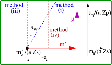
Figure 10: Results from different methods of defining maximal twist

.

Quenched simulations at $1/a\approx 2\;$GeV with unimproved Wilson fermions find an offset angle $\delta_{W}\approx-0.35$[70, 71]. This is a direct measure of discretization errors. Written as $a\Lambda^{2}$ this gives $\Lambda\approx 0.7\;$GeV, a large but not unreasonable value.

As noted above, the pion mass method can also be used, in principle, within the GSM regime. In practice the extrapolation can miss the critical mass, so it is useful to define a “straw-man” method (iv) in which $m^{\prime}$ is held fixed at a value of $O(a)$. As is clear from the figure, $\omega_{0}$ varies from $\sim 1$ to $0$ as $\mu$ varies from $\sim a$ to $0$. Thus one is never near maximal twist in the GSM regime, and automatic improvement is lost.

3.9 Results for $m_{q}\sim a^{2}\Lambda_{\rm QCD}^{3}$ (Aoki regime)

As discussed above, to describe simulations we need to extend the analysis into the Aoki regime. This requires a change in the power counting:[64, 59, 57] at LO we keep terms of size $m^{\prime}\sim\mu\sim a^{2}$,

$$\!{\mathcal{L}}_{\chi,Aoki}^{\rm LO}=\frac{{f}^{2}}{4}{\rm tr}(D_{\mu}\Sigma D_{\mu}\Sigma^{\dagger})\!-\!\frac{{f}^{2}}{4}{\rm tr}(\chi^{\prime\dagger}\Sigma\!+\!p.c.)\!-\!{W^{\prime}}\big{[}{\rm tr}(\hat{A}^{\dagger}\Sigma\!+\!p.c.)\big{]}^{2},$$ (91)

while at NLO we keep those of size $ma\sim\mu a\sim a^{3}$,

$$\!{\mathcal{L}}_{\chi,Aoki}^{\rm NLO}=-\frac{W_{3,1}}{f^{2}}{\rm tr}(\hat{A}^{\dagger}\hat{A}){\rm Tr}(\hat{A}^{\dagger}\Sigma+p.c.)-\frac{W_{3,3}}{f^{2}}\left[{\rm tr}(\hat{A}^{\dagger}\Sigma)^{3}+p.c.\right]$$ (92)

$$\!\!\!\!\!+{\widetilde{W}}{\rm tr}(D_{\mu}\Sigma^{\dagger}D_{\mu}\Sigma){\rm tr}(\hat{A}^{\dagger}\Sigma\!+p.c.)-{W}{\rm tr}(\chi^{\prime\dagger}\Sigma+p.c.){\rm tr}(\hat{A}^{\dagger}\Sigma\!+p.c.).$$

The two $a^{3}$ terms (those on the first line) are new, while previous NLO terms $\propto m^{2}$ become of NNLO. In fact, the $W_{3,1}$ term can be absorbed into $\chi^{\prime}$ by a further shift of $O(a^{4})$ in $m_{c}$. This leaves one new LEC at NLO, $W_{3,3}$. Note that only the source parts of the $W$ and $\widetilde{W}$ terms enter at NLO.

In the following I will describe the analysis of the phase structure at LO, and then mention some modifications caused by NLO terms.

The orientation of $\langle\Sigma\rangle$ is now determined by an equal competition between the mass and $a^{2}$ terms in $\mathcal{L}_{\chi,Aoki}^{\rm LO}$. The former is minimized when $\langle\Sigma\rangle\propto\chi^{\prime}\propto\exp(i\omega_{0}\tau_{3})$, while the latter either favors $\langle\Sigma\rangle=\pm 1$ ($W^{\prime}>0$) or $\langle\Sigma\rangle=\exp[i(\pi/2)\hat{n}\cdot\vec{\tau}]$ with $\hat{n}^{2}=1$ ($W^{\prime}<0$). The analysis along the Wilson axis is simple[41], and one finds two cases. Either the condensate jumps discontinuously from $\langle\Sigma\rangle=+1$ to $\langle\Sigma\rangle=-1$ at a first-order transition ($W^{\prime}>0$), or it swings between these values continuously, as is possible within $SU(2)$ ($W^{\prime}<0$). In the latter case, the condensate breaks flavor, so there are exact lattice Goldstone bosons. This is the Aoki phase[61]. The presence of two possible phase structures was also predicted by Creutz[72].

Moving into the twisted-mass plane the analysis becomes more complicated as one must minimize a quartic[53, 58, 55]. I show below how the two scenarios on the Wilson axis extend into the mass plane.

Here I use mass variables rescaled by $\sim a^{2}$:

$$\alpha=\frac{2B_{0}m^{\prime}}{(16{|W^{\prime}|}\hat{a}^{2}/f^{2})}=\frac{\hat{m^{\prime}}}{|w^{\prime}|}\,,\quad\beta=\frac{2B_{0}\mu}{(16{|W^{\prime}|}\hat{a}^{2}/f^{2})}=\frac{\hat{\mu}}{|w^{\prime}|}\,.$$ (93)

Both scenarios have a first-order transition boundary, indicated by the solid line, with second-order end-points. Note again that the parameter $w^{\prime}$, whose sign determines which scenario applies, and whose magnitude gives the size of the phase boundaries, is the same parameter as appears in the pion mass splitting[58], eq. (81). Thus a calculation of this splitting in the GSM regime (which, as noted above, has been attempted) predicts the phase structure in the Aoki regime.

Wu and I have given detailed plots of the condensate and pion masses along the dashed horizontal lines in the phase diagrams above[55]. I show here only a sample. I write the condensate as $\langle\Sigma\rangle=A_{m}+iB_{m}\tau_{3}$, and plot the scalar component $A_{m}$, as well as the charged and neutral pion mass-squareds. Figure 11 shows results for $W^{\prime}<0$. The “swinging” of the condensate between $\pm 1$, described in words above, is here the $\beta=0$ curve. The charged pion masses vanish when $|A_{m}|<1$, for then $|B_{m}|>0$ and flavor is spontaneously broken. Moving away from the Wilson axis ($\beta=1,2,3$), the Aoki-phase is washed out by the explicit breaking of flavor. The neutral pion (not shown) is always heavier than the charged pions.

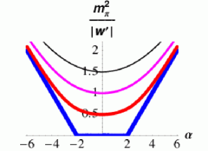
Figure 11: Condensate and charged pion masses for $W^{\prime}<0$, for four choices of twisted mass ($\beta=0,1,2,3$). The thickness of the lines decreases with increasing $\beta$.

If the mass is purely twisted ($\alpha=m^{\prime}=0$) then one finds for all $\beta$ that $A_{m}=0$, so the condensate points in the $\tau_{3}$ direction. Thus, despite the large discretization errors, the condensate ends up pointing in the same direction as it would without them. This is one way of understanding why automatic $O(a)$ improvement continues to work, as discussed further below.

I illustrate the results for the first-order scenario ($W^{\prime}>0$) in fig. 12. The left panel shows the discontinuity in the condensate for $|\beta|<2$, transforming into a smooth crossover for $|\beta|>2$. Above the transition, note again that $A_{m}=0$ when $\alpha=0$. The right panel shows that the pion mass on the Wilson axis ($\beta=0$) has a non-zero minimum, while for $\beta=2$ the neutral mass goes down to zero at the second-order end-point. In this scenario, the charged pions are always heavier than the neutral once one moves off the Wilson axis. Unlike the Aoki-phase scenario, however, no pions are massless along the phase boundary away from the end-points. This is because no lattice symmetry is broken along this transition.

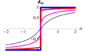
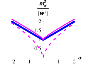
Figure 12: Condensate and pion masses for $W^{\prime}>0$. Notation as in fig. 11, except that pion masses are shown only for $\beta=0,2$. For $\beta=0$ charged and neutral pions are degenerate. For $\beta=2$, the neutral mass is shown dashed.

3.9.1 Applications to lattice simulations

(I) The most important lesson we learn from tm$\chi$PT is to expect non-trivial phase structure when $m_{q}\sim a^{2}$, with two possible scenarios. The prediction of an Aoki-phase was actually made long before the tm$\chi$PT analysis[61], in order to understand how $m_{\pi}^{2}$ could vanish without an underlying chiral symmetry, and quenched studies in the 1980’s and 90’s found evidence for such a phase. What has happened in the last few years is the beginning of detailed dynamical studies of the twisted-mass plane. Those with unimproved Wilson gauge and fermion actions found evidence for the first-order scenario. I think it is fair to say this was a surprise, and that it was predicted by $\chi$PT I view as a significant success. It is amusing that for decades we have been assuming that $m_{\pi}^{2}$ extrapolates all the way to zero, whereas (at least with the simplest actions) it actually never makes it.

I show an example of the evidence for the first-order scenario in Fig. 13. This shows scans at fixed twisted mass (with $\mu$ roughly fixed in physical units) for three lattice spacings ($a$ decreasing as $\beta$ increases). The plaquette and $m_{\rm PCAC}$ both have a discontinuity, and show hysteresis. Both effects decrease as one approaches the continuum limit, qualitatively consistent with expectations. The fact that $m_{\rm PCAC}$ has a minimum away from zero is a manifestation of the non-zero minimum in the pion masses.

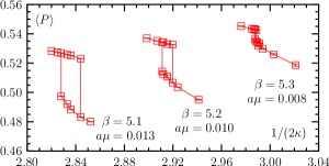
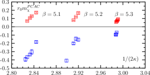
Figure 13: Average plaquette and $m_{\rm PCAC}$ plotted vs. $(2\kappa)^{-1}=m_{0}+4$ for fixed $\mu_{0}$[73].

(II) The predictions for physical quantities that I sketched above in the GSM regime have been extended to NLO in the Aoki regime[55, 64, 59, 57]. This is not trivial to implement, since minimization of the potential (with the $W_{3,3}$ term included) now involves a sextic equation. Detailed fits to quenched data have, however, been done, and find reasonable values for the resulting LECs[64].

I cannot resist showing one NLO prediction. Discretization effects distort the contours of constant $m_{\pi^{\pm}}^{2}$ from circles into the forms shown in fig. 14. Here $m^{\prime\prime}$ is just the shifted mass $m^{\prime}$ with the $O(a^{3})$ term proportional to $W_{3,1}$ absorbed as well. These plots are illustrative of the size of the expected effects, not the result of details fits. I have taken standard LO continuum LECs, and set the NLO continuum LECs and chiral logs to zero for simplicity. For the lattice LECs I use $\delta_{W}=\delta_{\widetilde{W}}=-0.3$, $|w^{\prime}|=(250\,{\textrm{M}eV})^{2}$ and $W_{3,3}=0$, values which are not unreasonable for $a^{-1}\approx 2\;$GeV. Quark masses range up to $\sim m_{s}/2$. Clearly the impact of discretization errors and phase structure could be very significant for actual simulation parameters.

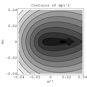
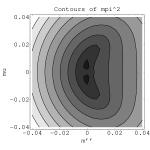
Figure 14: Contour plots of $m_{\pi^{\pm}}^{2}$ in twisted mass plane, for Aoki-phase (left) and first-order (right) scenarios, using a representative parameter set for $1/a\approx 2\;$GeV. Quark masses are in GeV. Raggedness in contours is due to numerical errors.

(III) Another important question that can be studied using tm$\chi$PT in the Aoki regime is whether automatic $O(a)$ improvement at maximal twist still holds using the criteria introduced in sec. 3.8. The answer is positive[56, 55, 59, 57], aside from a caveat I will explain. In fig. 15 I show the impact of NLO corrections on the phase boundaries and the lines of maximal twist[59]. These plots allow one to understand the qualitative features of the contours in fig. 14.

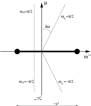
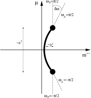
Figure 15: Phase diagram at NLO for Aoki-phase (left) and first-order (right) scenarios. Method (i) corresponds to $\omega_{A}=\pi/2$, method (iii) to $\omega_{P}=\pi/2$.

The lines of maximal twist shown in the figure are those for methods (i) and (iii). Along either line the physical quark mass is proportional to $\mu$. If one simulates on one of these lines, reducing $a$ while holding $\mu$ fixed (i.e. working at fixed physical quark mass), then the dependence of physical quantities on $a$ will be quadratic or of higher order. This is automatic $O(a)$ improvement. In the Aoki-phase scenario it holds even for $\mu\ll a^{2}$, i.e. all the way to the Wilson axis. For the first-order scenario the result breaks down, however, when one runs into the end-point with $\mu\approx|w^{\prime}|\sim a^{2}$. This is the caveat mentioned above.

It is perhaps surprising that one can work in a regime where the quark mass is much smaller than the leading $O(a)$ effects of discretization, and yet be able to tune parameters so these effects do not enter into physical quantities. It is worth understanding this qualitatively. The point is that the tuning has to be very fine. If $\mu\sim a^{2}$, then, as fig. 15 shows, one must tune $m^{\prime\prime}$ to an accuracy of $a^{3}$. This is what the criteria in eq. (88) accomplish. In terms of the Symanzik Lagrangian, this amounts to canceling the untwisted mass (so that it is $O(a^{3})$ or smaller). The result is

$${\mathcal{L}}^{(4+5)} = \overline{\psi}{\rm D}\!\!\!\!/\,\psi+\mu\overline{\psi}i\gamma_{5}\tau_{3}\psi+ac\overline{\psi}i\sigma_{\mu\nu}F_{\mu\nu}\psi+O(a^{2})$$ (94)

$$= \overline{\psi}_{\rm phys}{\rm D}\!\!\!\!/\,\psi_{\rm phys}+\mu\overline{\psi}_{\rm phys}\psi_{\rm phys}+ac\overline{\psi}_{\rm phys}\gamma_{5}\tau_{3}\sigma_{\mu\nu}F_{\mu\nu}\psi_{\rm phys}\,,$$ (95)

where in the second line I have rotated to the physical basis. The absence of a $\overline{\psi}\psi$ term on the first line means that the $O(a)$ term is purely flavor-parity breaking in the physical basis, and does not contribute to physical matrix elements however large it is. This is nothing more than a summary of the original argument for automatic improvement[43] (although simplified, as I am not including operators). The only new point here is that the argument goes through for arbitrarily small $\mu$ as long as $m^{\prime\prime}$ is tuned accurately enough.

It is now time to unveil what I call “method (ii)”, which works as follows. One first defines a critical mass by extrapolating results from method (i) to the Wilson axis, and then keeps $m_{0}$ fixed at this critical mass for all $\mu$. It turns out to correspond to working at $m^{\prime\prime}=0$. In the GSM regime (recall fig. 10) method (ii) is equivalent to method (iii), but in the Aoki regime the line it defines is offset from that of method (iii) by $O(a^{3})$. Such a difference might seem too small to be significant, but it need not be[57]. To see this, consider the Aoki-phase scenario. Then from fig. 15 one sees that method (ii) interpolates between method (i) ($\mu<a^{2}$) and method (iii) ($\mu\gg a^{2}$). Now, it turns out that the condensate has a fixed orientation as one moves along the lines of either method, but the orientations for the two methods differ by an angle of $O(a)$. Thus for method (ii) the condensate varies direction rapidly for $\mu\mathrel{\hbox to0.0pt{\lower 3.0pt\hbox{$\mathchar 536\relax$}\hss}\raise 2.0pt\hbox{$\mathchar 316\relax$}}a^{2}$, with a gradient of $\sim a/a^{2}$. This can disrupt extrapolations as the resulting form is not a simple polynomial[57]. I raise this worry because method (ii) is being used in practice by some groups, and it would be preferable to use method (i).

(IV) A further lesson from tm$\chi$PT is that both the size of the phase boundaries and the isospin splitting for pions are determined by the same parameter, $w^{\prime}$. It thus makes sense to try and tune the gauge and fermion actions to reduce $|w^{\prime}|$. Note that this tuning is not the same as a systematic improvement program, but it is nevertheless very important. Initial results in this direction are very encouraging. For example, fig. 16 shows that the discontinuities in the plaquette are significantly reduced by alternative gauge actions. It is also found that using an improved fermion action reduces the pion isospin splitting and thus $w^{\prime}$[67]. This is an active area of present research.

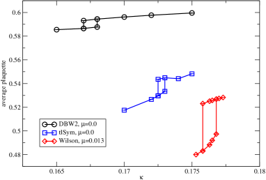
Figure 16: Hysteresis of plaquette at $a\approx 0.17\;$fm for DBW2 (top), tree-level improved Symanzik (middle) and Wilson (bottom) gauge actions.[74].

(V) It might appear from fig. 15 that, if we had to choose, we would prefer the Aoki-phase scenario because we can work at maximal twist down to $\mu=0$. I think, however, that the choice is not so clear. To illustrate why, I compare the results for pion masses in the two scenarios in fig. 17, using the same “reasonable” choices of LECs as above. The role of the charged and neutral pions is interchanged in the two scenarios, and there is no clear advantage to using one over the other. The figure also emphasizes the significance of the $O(a^{2})$ effects. I conclude that it is much more important to reduce the magnitude of $w^{\prime}$ than it is to end up in one or other scenario.

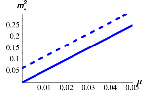
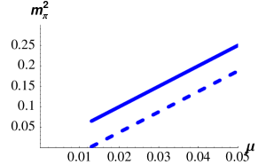
Figure 17: $m_{\pi^{\pm}}^{2}$ (solid) and $m_{\pi^{0}}^{2}$ (dashed) in GeV² versus $\mu$ in GeV for method (i). Left panel: Aoki-phase scenario; right panel: first-order scenario.

3.9.2 Bending near maximal twist

The discussion to this point makes clear the importance of accurate tuning to maximal twist. Initial studies of tmLQCD did not always attain this accuracy and observed a phenomenon called “bending”. Although this is largely a closed chapter in the history of tmLQCD, it is worth learning the appropriate lessons, particularly as tm$\chi$PT played an important role in elucidating the phenomenon.

The sketch to the right shows the Aoki-phase scenario with three choices of the approach to the chiral limit shown by arrows. They are all nominally at maximal twist. These are method (i) [thick lines]; fixing $m_{c}$ at an endpoint where $m_{\pi}=0$ [medium thickness], and missing the endpoint by $\sim a^{2}$ [thin lines].

I show in fig. 18 the NLO tm$\chi$PT results (using the same parameter set and assumptions as above) for $m_{\pi^{\pm}}^{2}/\mu$ for the three methods (with the thickness of the lines matching those above), along with results from simulations. The horizontal axis is $\mu$, which is the quark mass when working at maximal twist. For my parameters (i.e. physical LECs and chiral logs dropped) the correct result is a constant, and is illustrated by the $O(a)$ improved result from method (i) [thick line]. The results from the other two choices show a noticeable bending away from the continuum result at small masses, i.e. a breakdown of $O(a)$ improvement. The numerical results are for a similar range of quark masses, but the axes are in different units and so the two plots can only be compared qualitatively. The numerical results are for method (i) (“PCAC definition”—triangles) and the “$m_{\pi}=0$ definition” (circles), and are qualitatively consistent with tm$\chi$PT. A detailed fit of these and other quenched data to quenched tm$\chi$PT has been done, and finds quantitative agreement[64].

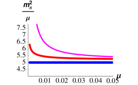
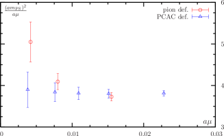
Figure 18: “Bending” in $m_{\pi}^{2}/\mu$ vs. $\mu$ from tm$\chi$PT[59] (left—both axes in GeV) and quenched simulations[44] (right—both axes in lattice units at $1/a\approx 2\;$GeV using bare $\mu$).

The most important conclusion from this figure is that one should use a good definition of maximal twist, such as method (i). In particular, the failure of the $m_{\pi}=0$ method is apparent. This can be understood qualitatively as follows. The condensate at maximal twist should lie in the $\tau_{3}$ direction, $\langle\Sigma\rangle=i\tau_{3}+O(a)$. This is the case with method (i). In the other cases, however, the condensate starts in this direction for $\mu\gg a^{2}$ but rotates away when $\mu\sim a^{2}$ and ends up at $\langle\Sigma\rangle=-1$ when $\mu=0$. Thus automatic $O(a)$ improvement is lost.

3.9.3 Does tmLQCD work in practice?

Tm$\chi$PT has been a very useful guide to the exploratory numerical studies of tmLQCD, but the most important question is whether working at maximal twist is practical. In particular, is the requisite fine tuning possible, and cheap enough, in practice? Are results for physical quantities really improved? These questions are being actively studied and the answers appear to be positive[44, 74, 75].

A different question is how best to include the strange quark, as one needs an even number of quarks to implement maximal twisting. One could just add a single non-perturbatively $O(a)$ improved untwisted strange quark to a maximally twisted up-down pair, but this would require non-perturbative improvement of each new operator involving the strange quark, which is exactly what we are trying to avoid with automatic improvement at maximal twist. An alternative is to introduce the charm quark as well, and treat the strange-charm pair as a twisted doublet[44]. Non-degenerate masses can be incorporated while maintaining maximal twist[76]. The disadvantages are that flavor breaking is more complicated (occurring in both $\tau_{3}$ and $\tau_{1}$ directions in the strange-charm sector), and that $(am_{c})^{2}$ effects may not be small. This option is being actively studied[77].

Finally, I think it likely that isospin breaking in pion masses will need to be included in loop calculations, requiring one to work at NNLO in the GSM power counting. First steps in this direction have been taken[78].

For further possible uses of tmLQCD, see the lectures by Sint.

4 Partial quenching and PQ$\chi$PT

My final lecture is devoted to introducing partially quenched QCD and the corresponding EFT, PQ$\chi$PT. I will consider PQQCD only in the continuum, and focus on conceptual issues. I will not discuss the extension to include discretization errors—this is straightforward following the methods of the previous lecture—nor the related topic of mixed action $\chi$PT. Nor will I discuss quenched QCD and quenched $\chi$PT (Q$\chi$PT), except in passing, as it is not useful for obtaining quantitative physical information about QCD.

4.1 What is PQQCD and why is it useful?

I have given an overview of the meaning of partial quenching in the introduction. Here I give a concrete example for the pion correlator in QCD. If we write out how this is calculated in detail,

$$C_{\pi}(\tau)=-\left\langle\sum_{\vec{x}}\overline{u}\gamma_{5}d(\vec{x},\tau)\ \overline{d}\gamma_{5}u(0)\right\rangle$$

$$\equiv -\frac{1}{Z}\int DU\prod_{q}DqD\overline{q}e^{-S_{\rm gauge}-\int_{x}\sum_{q}\overline{q}({\rm D}\!\!\!\!/\,+m_{q})q}\sum_{\vec{x}}\overline{u}\gamma_{5}d(\vec{x},\tau)\ \overline{d}\gamma_{5}u(0)$$

$$= \frac{1}{Z}\int DU\prod_{q}\det({\rm D}\!\!\!\!/\,\!+\!m_{q})e^{-S_{\rm gauge}}\sum_{\vec{x}}{\rm tr}\left[\gamma_{5}{\left(\frac{1}{{\rm D}\!\!\!\!/\,\!+\!m_{d}}\right)_{x0}}\gamma_{5}{\left(\frac{1}{{\rm D}\!\!\!\!/\,\!+\!m_{u}}\right)_{0x}}\right]$$

$\propto f_{\pi}^{2}e^{-m_{\pi}\tau}+\textrm{exponentially suppressed}$.

we see that, in practice, we are free to use different masses in the determinant (“sea” or “dynamical” quark masses) and in the propagators (“valence” quark masses). Doing so is called partial quenching. It is relatively cheap to do so, since the calculation of propagators is usually a small overhead on the generation of configurations, thanks to the determinant, and because the rate of increase of CPU time as $m_{q}$ decreases is less severe for propagators. The big question is whether we can make use of the extra information provided by working with $m_{\rm val}\neq m_{\rm sea}$.

At this point it is appropriate to interject a comment on nomenclature. In the bad old days we used the quenched approximation, in which $m_{\rm sea}\to\infty$, so the quark determinant could be ignored. This allowed simulations to be done, but at the heavy cost of ignoring quark loops and thus considering a theory which is not unitary and had various sicknesses. QQCD is at best a model of QCD—there is no quantitative relation between the two theories. Partial quenching is in one sense a less extreme version of quenching, and thus the name. If $m_{\rm sea}\gg\Lambda_{\rm QCD}$ then PQQCD, like QQCD, is only qualitatively related to QCD, and the name is appropriate. What I consider here, however, is PQQCD with sea quarks light enough, $m_{\rm sea}\ll\Lambda_{\rm QCD}$, that (as I will argue) we can use $\chi$PT to relate the results quantitatively to physical QCD. For such theories a more appropriate name, with less negative connotations, would be “partially unquenched”. But I will not try and create a naming revolution and will stick with the canonical nomenclature.

One thing that having light sea quarks does not change is that PQQCD is unphysical. To see this consider a contribution to $\pi^{0}\pi^{0}$ scattering in QCD: the two pions first annihilate into glue, from which is created, say, a $\pi^{+}\pi^{-}$ intermediate state, which subsequently annihilates back into glue, and then finally a new $\pi^{0}$ pair is created. In the corresponding process in PQQCD, the intermediate $\pi^{+}\pi^{-}$ pair must be composed of sea quarks, and thus have different masses from the valence $\pi^{0}$ pairs. Having different intermediate and external states means that the theory is not unitary. Another unphysical feature is the appearance of double poles in propagators. This is not possible if one can insert a complete set of physical states. The fact that there are double poles can be seen in PQ$\chi$PT[79], but can also be seen more generally from the properties of the quark-level theory[80].

Because PQQCD is unphysical, it is essential to have a quantitative method relating its properties to those of QCD. This is provided by PQ$\chi$PT. Thus we must simulate in the regime of quark masses where $\chi$PT is valid if PQQCD is to be a useful tool. This is illustrated above in fig. 1. Note that the presence of the physical subspace with $m_{\rm val}=m_{\rm sea}$ within PQQCD is crucial in order to pin down the relation to QCD.

4.2 A field theoretic formulation of PQQCD

As we have seen, the construction of an EFT makes essential use of symmetries. Thus to develop PQ$\chi$PT we need a formulation of PQQCD which makes its symmetries manifest. One way to do this is to use Morel’s trick[81] of introducing commuting spin-$1/2$ fields (ghost quarks labeled $\widetilde{q}$), whose determinant can cancel that from the valence quarks:

$$\!\!\int\!\!D\overline{q}Dqe^{-\overline{q}({\rm D}\!\!\!\!/\,\!+\!m_{q})q}\!=\!\mathrm{det}({\rm D}\!\!\!\!/\,\!+\!m_{q})\,,\ \int\!\!D\widetilde{q}^{\dagger}D\widetilde{q}e^{-\widetilde{q}^{\dagger}({\rm D}\!\!\!\!/\,\!+\!m_{q})\widetilde{q}}\!=\!\frac{1}{\mathrm{det}({\rm D}\!\!\!\!/\,\!+\!m_{q})}\,.$$ (97)

The formulation then includes three types of quark: valence quarks $q_{V1}$, $q_{V2}$, …$q_{VN_{V}}$, ($N_{V}=2,3,\dots$), sea quarks $q_{S1}$, $q_{S2}$, …$q_{SN}$ ($N=2,3$), and ghost quarks $\widetilde{q}_{V1}$, $\widetilde{q}_{V2}$, …$\widetilde{q}_{VN_{V}}$ ($N_{V}=2,3,\dots$). The ghosts are degenerate with corresponding valence quarks. It is notationally convenient to package these fields into $(N+2N_{V})$-dim vectors:

$$Q^{tr}=\bigg{(}\underbrace{{q_{V1}},\dots,{q_{VN_{V}}}}_{\rm valence},\,\underbrace{{q_{S1}},\dots,{q_{SN}}}_{\rm sea},\,\underbrace{{\widetilde{q}_{V1}},\dots,{\widetilde{q}_{VN_{V}}}}_{\rm ghost}\bigg{)}\,,$$ (98)

$$\overline{Q}=\bigg{(}\underbrace{{\overline{q}_{V1}},\dots,{\overline{q}_{VN_{V}}}}_{\rm valence},\,\underbrace{{\overline{q}_{S1}},\dots,{\overline{q}_{SN}}}_{\rm sea},\,\underbrace{{\widetilde{q}_{V1}^{\dagger}},\dots,{\widetilde{q}_{VN_{V}}^{\dagger}}}_{\rm ghost}\bigg{)}\,,$$ (99)

and similarly for the masses

$${\mathcal{M}}=\bigg{(}\underbrace{{m_{V1}},\dots,{m_{VN_{V}}}}_{\rm valence},\,\underbrace{{m_{S1}},\dots,{m_{SN}}}_{\rm sea},\,\underbrace{{m_{V1}},\dots,{m_{VN_{V}}}}_{{\rm ghost}={\rm valence}}\bigg{)}\,.$$ (100)

The action of PQQCD is a simple extension of that of QCD

$$S_{\rm PQ} = S_{\rm gauge}+\int\overline{Q}({\rm D}\!\!\!\!/\,+{\mathcal{M}})Q$$ (101)

$$\overline{Q}({\rm D}\!\!\!\!/\,+{\mathcal{M}})Q = \sum_{i=1}^{N_{V}}{\overline{q}_{Vi}({\rm D}\!\!\!\!/\,+m_{Vi})q_{Vi}}+\sum_{j=1}^{N}{\overline{q}_{Sj}({\rm D}\!\!\!\!/\,+m_{Sj})q_{Sj}}$$ (102)

$$\mbox{}\qquad+\sum_{k=1}^{N_{V}}{\widetilde{q}_{Vk}^{\dagger}({\rm D}\!\!\!\!/\,+m_{Vk})\widetilde{q}_{Vk}}\,.$$

If we similarly define an extended measure as

$$D\overline{Q}DQ\equiv\prod_{i=1}^{N_{V}}\left({D\overline{q}_{Vi}Dq_{Vi}}{D\widetilde{q}_{Vi}^{\dagger}D\widetilde{q}_{Vi}}\right)\prod_{j=1}^{N}\left({D\overline{q}_{Sj}Dq_{Sj}}\right)\,,$$ (103)

then we can write down a partition function containing valence quarks that nevertheless reproduces that of QCD:

$$Z_{\rm PQ} = \int DUD\overline{Q}DQ\ e^{-S_{\rm PQ}}$$ (104)

$$= \int DUe^{-S_{\rm gauge}}\prod_{i=1}^{N_{V}}\left(\frac{{\mathrm{det}({\rm D}\!\!\!\!/\,+m_{Vi})}}{{\mathrm{det}({\rm D}\!\!\!\!/\,+m_{Vi})}}\right)\prod_{j=1}^{N}{\mathrm{det}({\rm D}\!\!\!\!/\,+m_{Sj})}$$ (105)

$$= \int DUe^{-S_{\rm gauge}}\prod_{j=1}^{N}{\mathrm{det}({\rm D}\!\!\!\!/\,+m_{Sj})}=Z_{\rm QCD}$$ (106)

So far this is rather trivial. The power of the method is that it provides field-theoretic expressions for PQ correlation functions, e.g.

$$\!\!\!\!\!\!\!C_{\pi}^{\rm PQ}(\tau) \equiv -Z_{\rm PQ}^{-1}\int DUD\overline{Q}DQ\ e^{-S_{\rm PQ}}\sum_{\vec{x}}{\overline{u}_{V}}\gamma_{5}{d_{V}}(\vec{x},\tau)\ {\overline{d}_{V}}\gamma_{5}{u_{V}}(0)$$ (108)

$$= Z_{\rm PQ}^{-1}\int DU\prod_{j=1}^{N}{\det({\rm D}\!\!\!\!/\,+m_{Sj})}e^{-S_{\rm gauge}}$$

$$\mbox{}\qquad\times\sum_{\vec{x}}{\rm tr}\left[\gamma_{5}{\left(\frac{1}{{\rm D}\!\!\!\!/\,+m_{Vd}}\right)_{x0}}\gamma_{5}{\left(\frac{1}{{\rm D}\!\!\!\!/\,+m_{Vu}}\right)_{0x}}\right]\,.$$

This is exactly the pion correlator with which we started, eq. (4.1), but with differing valence and sea quark masses.

As noted above, PQQCD is “anchored” to QCD (or, more precisely, to physical, QCD-like, theories). Let us see how this works in our new formulation. Consider the PQ pion correlator, but now set the valence quark masses equal to two of the sea quark masses, i.e. ${m_{Vu}}={m_{Sj}}$ and ${m_{Vd}}={m_{Sk}}$. Then the PQ correlator is equal to a physical QCD correlator:

$$\!\!\!\!C_{\pi}^{\rm PQ}(\tau) = Z_{\rm PQ}^{-1}\int DUD\overline{Q}DQ\ e^{-S_{\rm PQ}}\sum_{\vec{x}}{\overline{u}_{V}}\gamma_{5}{d_{V}}(\vec{x},\tau)\ {\overline{d}_{V}}\gamma_{5}{u_{V}}(0)$$ (109)

$$= Z_{\rm PQ}^{-1}\int DUD\overline{Q}DQe^{-S_{\rm PQ}}\sum_{\vec{x}}{\overline{q}_{Sj}}\gamma_{5}{q_{Sk}}(\vec{x},\tau)\ {\overline{q}_{Sk}}\gamma_{5}{q_{Sj}}(0)$$ (111)

$$= Z_{\rm QCD}^{-1}\int DU\prod_{i=1}^{N}{D\overline{q}_{Si}Dq_{Si}}\ e^{-S_{\rm QCD}}$$

$$\mbox{}\qquad\qquad\qquad\qquad\times\sum_{\vec{x}}{\overline{q}_{Sj}}\gamma_{5}{q_{Sk}}(\vec{x},\tau)\ {\overline{q}_{Sk}}\gamma_{5}{q_{Sj}}(0)$$

$$= C_{\pi}^{\rm QCD}(\tau)\,.$$ (112)

To obtain the second line I used the result that the propagators obtained by doing the Wick contractions are the identical to those from the first line. This is an example of the enlarged symmetry of the PQ theory. Having removed the valence quarks from the operators, the valence and ghost integrals cancel, leaving a QCD correlation function. This analysis generalizes to any correlation function containing $N$ or less different valence quark-antiquark pairs (recall that we can add any number of valence quarks). If there are more than $N$ such pairs, e.g. a two point function containing $\overline{q}_{V1}q_{V2}\overline{q}_{V3}q_{V4}$ and its conjugate in the presence of 3 light sea quarks, then there is no corresponding QCD correlator even if valence masses are all equal to sea masses. This is an example, developed further below, of how PQQCD gives one access to combinations of Wick contractions that do not occur in QCD itself.

The field theoretic formulation shows that PQQCD is a well-defined statistical system. In particular, the ghosts do not present a theoretical problem in the Euclidean functional integral. As long as quark masses are positive, the functional integrals over the ghost quarks converge (since ${\rm D}\!\!\!\!/\,$ has imaginary eigenvalues). Of course, the theory remains unphysical, and indeed we can now see this more directly. If we rotate to Minkowski space we will violate the spin-statistics theorem, and thus have an unphysical theory. Put another way, PQQCD does not satisfy reflection positivity (as can be seen, for example, from the fact that the ghost pion correlator has the opposite sign to that for the normal pion), and so one cannot construct a physical Hilbert space with a positive Hamiltonian. But the unphysical nature need not be a problem if we use PQQCD in Euclidean space as a tool to gain information about QCD.

4.3 Developing PQ$\chi$PT

Before diving into the theoretical details let me give some qualitative motivation for what follows. We will need to assume that PQQCD is described by an effective theory close to that for QCD. I think it is fair to say that our confidence in this assumption is based in part on results from simulations. In particular, the charged pion correlator, $C_{\pi}^{\rm PQ}(\tau)$, has essentially the same form at long distances in PQQCD (and also QQCD) as in QCD: it falls as $\exp(-m_{\pi}\tau)$ at long times, and $m_{\pi}^{2}\propto(m_{Vu}+m_{Vd})$ to good approximation. There is no sign of unphysical effects, e.g. double poles [which fall as $t\exp(-m_{\pi}t)$], or negative residues. It is only when one looks in detail that one finds deviations from QCD expectations, such as the enhanced chiral logarithms in QQCD. There are also other correlators where partial quenching has a dramatic effect: double poles do appear in the $\eta^{\prime}$ correlator, and there are negative contributions to the scalar-isovector correlator. Nevertheless, the apparent closeness of the infrared physics of PQQCD to that of QCD provides important motivation for the development of (P)Q$\chi$PT.

This development has been done using two methods. The first is the “graded-symmetry” method[79] based on Morel’s trick and which I use here. This is an extension of earlier work on the quenched theory[82]. The main issue, as we will see, is the whether the usual “derivation” of an EFT goes through when the theory is unphysical. The second method uses the “replica-trick”[83], in which one removes the valence determinant by sending $N_{V}\to 0$ rather than using ghosts. This has the advantage that the theories with integer $N_{V}$, from which one is extrapolating, are physical, and so one expects their long-distance physics to be described by $\chi$PT. Its disadvantage is that extrapolating in $N_{V}$ is, in general, theoretically uncontrolled.

For the purposes of the present lecture I could use either method, since they are known to give the same results at one-loop in PQ$\chi$PT, and it is plausible that this holds to all orders[83]. I choose the graded-symmetry method as I am more familiar with it.

4.3.1 Symmetries of PQQCD

In the notation developed above, $S_{\rm PQQCD}=S_{\rm gauge}+\overline{Q}({\rm D}\!\!\!\!/\,+{\mathcal{M}})Q$ looks just like $S_{\rm QCD}$, and appears to have a graded extension of chiral symmetry when $\mathcal{M}\to 0$, involving rotation of quarks into ghosts and vica-versa:

$$Q_{L,R}\longrightarrow{U_{L,R}}Q_{L,R}\,,\ \overline{Q}_{L,R}\longrightarrow\overline{Q}_{L,R}{U_{L,R}^{\dagger}}\,,\ {U_{L,R}\in SU(N_{V}+N|N_{V})}.$$ (113)

The apparent symmetry is $SU(N_{V}+N|N_{V})_{L}\times SU(N_{V}+N|N_{V})_{R}\times U(1)_{V}$. In fact, there are subtleties in the ghost sector: the transformations are inconsistent with the requirement that $\overline{Q}$ contain $\widetilde{q}_{V}^{\dagger}$ in the ghost sector (and thus is related to $Q$, unlike in the quark sectors). This is necessary for convergence of the ghost functional integral[86]. I do not have space to discuss this technical detail, and I refer the interested reader to the literature[86, 87, 80, 88]. The bottom line is that, for perturbative calculations in the EFT, one gets the same answer using the apparent symmetry group.

4.3.2 Brief primer on graded Lie groups

Since these are lectures, I recall a few basic properties of graded Lie groups. Graded means that the group matrices, $U$, contain both commuting and anticommuting elements

$$U=\left(\begin{array}[]{cc}A&B\\ \underbrace{C}_{N_{V}+N}&\underbrace{D}_{N_{V}}\end{array}\right)\quad\textrm{{$A,D$} commuting; {$B,C$} anticommuting}\,.$$ (114)

$U$ is unitary [i.e. $U\in U(N_{V}+N|N_{V})$] if $UU^{\dagger}=U^{\dagger}U=1$, as for normal matrices, as long as one complex conjugates anticommuting variables as $(\eta_{1}\eta_{2})^{*}\equiv\eta_{2}^{*}\eta_{1}^{*}$. Trace is generalized to “supertrace”, defined to maintain cyclicity:

$${\rm str}\;U\equiv{\rm tr}A-{\rm tr}D\quad\Rightarrow\quad{\rm str}(U_{1}U_{2})={\rm str}(U_{2}U_{1})\,.$$ (115)

Determinants generalize to “superdeterminants”,

$${\rm sdet}\;U\equiv\exp[{\rm str}(\ln U)]={\det(A-BD^{-1}C)}/{\det(D)}\,,$$ (116)

which satisfy ${\rm sdet}(U_{1}U_{2})={\rm sdet}(U_{1}){\rm sdet}(U_{2})$. Using this one can define $U\in SU(N_{V}+N|N_{V})$ as unitary graded matrices with unit superdeterminant.

To get a feel for the subtleties of the graded groups it is useful to consider examples of $SU(N_{V}+N|N)$ matrices:

$$\!\!U_{I} = \left(\begin{array}[]{cc}SU(N_{V}+N)&0\\ 0&SU(N_{V})\end{array}\right)\quad\Rightarrow\quad{\rm sdet}\;U_{I}=1\,,$$ (119)

$$\!\!U_{II} = \left(\begin{array}[]{cc}e^{i\theta N_{V}}&0\\ 0&e^{i\theta(N+N_{V})}\end{array}\right)\ \ \Rightarrow\ \ {\rm sdet}\;U_{II}=\frac{(e^{i\theta N_{V}})^{N+N_{V}}}{(e^{i\theta(N+N_{V})})^{N_{V}}}=1\,.$$ (122)

$U_{I}$ looks just like an $SU(2N_{V}+N)$ matrix, while $U_{II}$ does not (having a determinant differing from unity). Its superdeterminant is unity thanks to the $\det(D)$ in the denominator of (116).

One feature of $U(N_{V}+N|N_{V})$ which is unchanged from ungraded groups is that one can pull out a commuting $U(1)$ factor, $U(N_{V}+N|N_{V})=[SU(N_{V}+N|N_{V})\otimes U(1)]/Z_{N}$, with the $U(1)$ being a phase rotation:

$$U_{III}=\left(\begin{array}[]{cc}e^{i\theta}&0\\ 0&e^{i\theta}\end{array}\right)\quad\Rightarrow\quad{\rm sdet}\;U_{III}=\frac{e^{i\theta(N+N_{V})}}{e^{i\theta N_{V}}}=e^{i\theta N}\,.$$ (123)

4.3.3 Chiral symmetry breaking

We now follow the same steps as we did for QCD in sec. 2.2, noting differences along the way. We expand PQQCD about ${\mathcal{M}}=0$, where the chiral symmetry group ${G}=SU(N_{V}+N|N_{V})_{L}\times SU(N_{V}+N|N_{V})_{R}$ is exact. We know that this symmetry is broken, because it is broken in the massless QCD contained in massless PQQCD. To study the symmetry breaking we introduce a graded generalization of the order parameter (6) used for QCD:

$$\Omega_{ij}=\langle Q_{L,i,\alpha,c}\overline{Q}_{R,j,\alpha,c}\rangle_{\rm PQ}\ {\lower 2.58334pt\hbox{$\stackrel{{\scriptstyle G}}{{\longrightarrow}}$}}\ U_{L}\,\Omega\,U_{R}^{\dagger}\,.$$ (124)

Next we assume that the graded vector symmetry, $SU(N_{V}+N|N_{V})_{V}$, is not spontaneously broken. If ${\mathcal{M}}$ is diagonal, real and positive, this follows from an extension[80] of the Vafa-Witten theorem for QCD[23]. The assumption is thus that nothing singular happens as $\mathcal{M}\to 0$. Given this, we know that $\Omega=\omega\times{\bf 1}$, and, furthermore, we know from the QCD sub-theory that $\omega={\langle q_{S}\overline{q}_{S}\rangle}\neq 0$. Thus the symmetry breaking is ${G}\to{H}=SU(N_{V}+N|N_{V})_{V}$, a simple graded generalization of that in QCD.

We can now derive Goldstone’s theorem using Ward identities for two-point Euclidean correlators, which remain exact in the PQ theory[80]. The result is that there are massless, spinless poles which couple to $\overline{Q}\gamma_{\mu}\gamma_{5}T^{a}Q$ for all $(N+2N_{V})^{2}-1$ traceless generators, $T^{a}$, of $SU(N_{V}+N|N_{V})$. Of these, $2(N+N_{V})N_{V}$ are fermionic (quark-ghost particles), $(N+N_{V})^{2}-1$ are bosonic with normal sign two-point functions (quark-quark), and $N_{V}^{2}$ are bosonic with unphysical sign two-point functions (ghost-ghost).

4.3.4 Constructing the EFT

It would appear that we have the ingredients to construct an EFT, just as in QCD: we know the symmetries, and we have a separation of scales. In fact, we know much less than in QCD, because PQQCD is not physical. In QCD, the poles in two-point functions correspond to particle states in a physical Hilbert space, and thus we know that correlation functions of arbitrary order will also have these poles, and from their residues we can extract the S-matrix, which will be unitary. Furthermore, since QCD involves local interactions, the S-matrix will satisfy cluster decomposition. Then we can invoke Weinberg’s “theorem” and write an effective, local field theory for the light particles. In PQQCD, by contrast, we do not know that the poles we have found in two-point functions also appear in higher order correlators, and we do know that there is neither a physical Hilbert space nor S-matrix. Indeed, it can be shown that neutral correlators have double-poles if $m_{V}\neq m_{S}$[80]. So we cannot rely on Weinberg’s argument. Instead we must simply assume that there is a local EFT containing the Goldstone modes and satisfying the symmetries. In other words we assume a minimal change from the EFT for QCD.

This is not as ad hoc as it might sound. Let me give three arguments in favor of this assumption. First, we know that there is a local EFT for the QCD sub-theory, and that this describes the long distance behavior of correlators. What PQQCD allows one to do is to separate individual Wick contractions contributing to QCD correlators. It seems implausible that, for example, the description of these individual contractions would require a non-local interaction (leading to a different pole structure) whose effects cancel when one adds them to form QCD correlators. Second, one can derive chiral Ward identities in PQQCD for arbitrary order correlation functions, that are generalizations of those in QCD. PQ$\chi$PT satisfies these identities by saturating them with Goldstone pole contributions. In this regard, there is numerical evidence from simulations that in, say, four-point functions the Goldstone poles dominate when one pulls one of the operators far from the others, as predicted by PQ$\chi$PT. Finally, one can imagine carrying out a Wilsonian renormalization group program in a Euclidean theory, in which one successively integrates out “shells” of high-momentum modes. This automatically leads to a local interaction, and symmetries are preserved. One can think of Symanzik’s EFT for lattice QCD as an example. We cannot actually do the calculation here, given the non-perturbative physics of QCD, but if we could, and if the two-point functions correctly tell us the appropriate low-energy degrees of freedom, it is plausible that we would end up with PQ$\chi$PT.

Having assumed the nature of the EFT we continue following the same steps as for QCD. We “promote” the condensate into a field,

$$\Omega/\omega\to\Sigma(x)\in SU(N_{V}+N|N)\,,\qquad\Sigma\stackrel{{\scriptstyle G}}{{\longrightarrow}}U_{L}\,\Sigma\,U_{R}^{\dagger}\,,$$ (125)

and, assuming standard masses so that $\langle\Sigma\rangle=1$, we define NG particles by

$$\Sigma=\exp\left[\frac{2i}{f}\Phi(x)\right]\,,\qquad\Phi(x)=\left(\begin{array}[]{cc}\phi(x)&\eta_{1}(x)\\ \eta_{2}(x)&\widetilde{\phi}(x)\end{array}\right)\,.$$ (126)

Here $\phi$ are the quark-quark “normal” NG bosons, $\widetilde{\phi}$ are the ghost-ghost NG bosons, and $\eta_{1,2}$ are quark-ghost NG fermions. The constraint ${\rm sdet}\;\Sigma=1$ implies ${\rm str}\;\Phi={\rm tr}\;\phi-{\rm tr}\;\widetilde{\phi}=0$. The QCD part of $\Sigma$ is

$$\Phi(x)=\left(\begin{array}[]{ccc}0&0&0\\ 0&\pi(x)&0\\ \underbrace{0}_{N_{V}}&\underbrace{0}_{N}&\underbrace{0}_{N_{V}}\end{array}\right)\quad\Rightarrow\quad\Sigma=\left(\begin{array}[]{ccc}1&0&0\\ 0&\Sigma_{\rm QCD}&0\\ 0&0&1\end{array}\right)\,.$$ (127)

Next we construct the most general local, Euclidean-invariant, $G$-invariant Lagrangian built out of $\Sigma$, $D_{\mu}\Sigma$ and $\chi$. Here the covariant derivative and $\chi$ are graded generalizations of the corresponding terms in $\chi$PT. In particular $\chi=2B_{0}(s+ip)\to U_{L}\chi U_{R}^{\dagger}$, with the sources set to $s=\mathcal{M}$ and $p=0$ at the end. We can use generalizations of the same building blocks as in $\chi$PT, e.g.

$$L_{\mu}=\Sigma D_{\mu}\Sigma^{\dagger}\to U_{L}L_{\mu}U_{L}^{\dagger}\,,\quad{\rm str}(L_{\mu})=0\,,\quad$$ (128)

The power counting (which is independent of the nature of the fields) is the same as in $\chi$PT.

In this way we arrive at the PQ chiral Lagrangian through NLO:

$${\mathcal{L}}_{\rm PQ}^{(2)} = \frac{f^{2}}{4}{\rm str}\left(D_{\mu}\Sigma D_{\mu}\Sigma^{\dagger}\right)-\frac{f^{2}}{4}{\rm str}(\chi\Sigma^{\dagger}+\Sigma\chi^{\dagger})$$ (129)

$${\mathcal{L}}_{\rm PQ}^{(4)} = -{L_{1}}\,\big{[}{\rm str}(D_{\mu}\Sigma D_{\mu}\Sigma^{\dagger})\big{]}^{2}-{L_{2}}\,{\rm str}(D_{\mu}\Sigma D_{\nu}\Sigma^{\dagger}){\rm str}(D_{\mu}\Sigma D_{\nu}\Sigma^{\dagger})$$ (130)

$$+{L_{3}}\,{\rm str}(D_{\mu}\Sigma D_{\mu}\Sigma^{\dagger}D_{\nu}\Sigma D_{\nu}\Sigma^{\dagger})$$

$$+{L_{4}}\,{\rm str}(D_{\mu}\Sigma^{\dagger}D_{\mu}\Sigma){\rm str}(\chi^{\dagger}\Sigma\!+\!\Sigma^{\dagger}\chi)+{L_{5}}\,{\rm str}(D_{\mu}\Sigma^{\dagger}D_{\mu}\Sigma[\chi^{\dagger}\Sigma\!+\!\Sigma^{\dagger}\chi])$$

$$-\!{L_{6}}\big{[}{\rm str}(\chi^{\dagger}\Sigma\!+\!\Sigma^{\dagger}\chi)\big{]}^{2}\!-\!{L_{7}}\big{[}{\rm str}(\chi^{\dagger}\Sigma\!-\!\Sigma^{\dagger}\chi)\big{]}^{2}\!-\!{L_{8}}\,{\rm str}(\chi^{\dagger}\Sigma\chi^{\dagger}\Sigma\!+\!p.c.)$$

$$+i{L_{9}}\,{\rm str}(L_{\mu\nu}D_{\mu}\Sigma D_{\nu}\Sigma^{\dagger}\!+\!p.c.)+{L_{10}}\,{\rm str}(L_{\mu\nu}\Sigma R_{\mu\nu}\Sigma^{\dagger})$$

$$+{H_{1}}\,{\rm str}(L_{\mu\nu}L_{\mu\nu}+p.c.)-{H_{2}}\,{\rm str}(\chi^{\dagger}\chi)+\mathcal{L}_{\rm WZW,PQ}$$

$${+L_{\rm PQ}{\mathcal{O}}_{PQ}}\,.$$

These are almost carbon copies of the corresponding results in $\chi$PT [eqs. (28,31)], except that ${\rm tr}\to{\rm str}$, and there is an additional term in $\mathcal{L}_{\rm PQ}^{(4)}$ (the ${\mathcal{O}}_{\rm PQ}$ term)[90]. To my knowledge, no-one has worked out the structure of the PQ WZW term in detail, though its contributions to $\pi^{0}\to\gamma\gamma$ vertices have been analyzed[91].

Thus we find that the number of LECs in PQ$\chi$PT is the same as in $\chi$PT at LO, and that there is only one more, $L_{\rm PQ}$, at NLO. But how are these LECs related to those of $\chi$PT? The answer is simple[6]: they are the same! This can be seen by considering correlation functions created by sources $s,p,l_{\mu},r_{\mu}$ restricted to the QCD sub-space. At the quark level, these are QCD correlators, since valence and ghost contributions cancel identically. Thus they are described by $\chi$PT. At the EFT level, one can show diagramatically in PQ$\chi$PT that a similar cancellation occurs, and that one can do the calculation using $\Sigma$ restricted to the QCD subspace as in (127). Inserting this form into $\mathcal{L}_{\rm PQ}^{(2,4)}$ one finds ($i=1,10$, HEC ignored):

$${\mathcal{L}}_{{\rm PQ}}^{(2,4)}(\Sigma,L_{i},L_{\rm PQ})={\mathcal{L}}^{(2,4)}(\Sigma_{\rm QCD},L_{i})\,.$$ (131)

In words, the calculation one does with QCD sources in PQ$\chi$PT is exactly that one would do in $\chi$PT. For the results to be equal it must be that the $L_{i}$ are equal. This is the key result in PQ$\chi$PT, for it means that the predictions of PQ$\chi$PT involve only slightly more LECs than those of $\chi$PT.

4.3.5 What about ${\mathcal{O}}_{\rm PQ}$?

Back when we were constructing ${\mathcal{L}}^{(4)}$ in $\chi$PT, I noted that one possible four-derivative term was not independent for $N\leq 3$. This is due to Cayley-Hamilton relations between traces of finite matrices. Such relations do not hold for graded matrices, and so the term is independent in PQ$\chi$PT. It is convenient to write it as

$${\mathcal{O}}_{\rm PQ} = {\rm str}(D_{\mu}\Sigma D_{\nu}\Sigma^{\dagger}D_{\mu}\Sigma D_{\nu}\Sigma^{\dagger})+2\;{\rm str}(D_{\mu}\Sigma D_{\nu}\Sigma^{\dagger}D_{\mu}\Sigma D_{\nu}\Sigma^{\dagger})$$ (132)

$$\mbox{}-{\rm str}(D_{\mu}\Sigma D_{\mu}\Sigma^{\dagger})^{2}/2-{\rm str}(D_{\mu}\Sigma D_{\nu}\Sigma^{\dagger}){\rm str}(D_{\mu}\Sigma D_{\nu}\Sigma^{\dagger})\,,$$

for then it vanishes if $\Sigma$ is restricted to its QCD subspace as in (127). This is why $L_{\rm PQ}$ does not appear on the right-hand side of eq. (131). ${\mathcal{O}}_{\rm PQ}$ does not vanish for general $\Sigma$, however, and thus appears in ${\mathcal{L}}_{{\rm PQ}}^{(4)}$ with a new LEC. This additional LEC also appears in standard $\chi$PT if $N\geq 4$, when the Cayley-Hamilton relations become less restrictive. As one goes to higher order, the number of additional such operators in PQ$\chi$PT increases[90].

How does this new operator enter into results for measurable quantities in PQQCD? It can only contribute to PQ quantities, for the considerations above show that it vanishes when restricted to the QCD sub-space. It turns out to contribute to PQ $\pi\pi$ scattering at NLO, but to PQ $m_{\pi}$ and $f_{\pi}$ only at NNLO[90]. Thus its practical impact is small.

It is worthwhile, however, understanding its origin more deeply. As I have repeatedly mentioned, PQQCD allows one to separate individual Wick contractions, unlike QCD. For example, $\pi^{+}K^{0}$ scattering in QCD has two contractions (thin [blue] is $u$, medium [red] is $d$, and thick [brown] is $s$):

and ${\mathcal{O}}_{\rm PQ}$ makes no contribution to this process. We can separate these contractions in PQQCD using, for example, scattering involving ghost quarks:

This is the same as the first contraction contributing to QCD scattering, up to a sign. ${\mathcal{O}}_{\rm PQ}$ does contribute to this correlator. Thus $L_{\rm PQ}$ contains information about the relative size of two contractions in the QCD process.

4.4 PQ$\chi$PT at LO

With the Lagrangian in hand it is straightforward to develop perturbation theory. Inserting the expansion (126) into $\mathcal{L}_{\rm PQ}^{(2)}$, we find

$$\!\!\!{\mathcal{L}}_{\rm PQ}^{(2)} = {\rm str}(\partial_{\mu}\Phi\partial_{\mu}\Phi)+{\rm str}(\chi\Phi^{2})+\dots$$ (136)

$$= {\rm tr}(\partial_{\mu}\phi\partial_{\mu}\phi+\partial_{\mu}\eta_{1}\partial_{\mu}\eta_{2}-\partial_{\mu}\eta_{2}\partial_{\mu}\eta_{1}-\partial_{\mu}\widetilde{\phi}\partial_{\mu}\widetilde{\phi})$$

$$\mbox{}\!\!\!+{\rm tr}\left[(\phi^{2}+\eta_{1}\eta_{2})\left(\begin{array}[]{cc}\chi_{V}&0\\ 0&\chi_{S}\end{array}\right)\right]-{\rm tr}(\widetilde{\phi}^{2}\chi_{V})-{\rm tr}(\eta_{2}\eta_{1}\chi_{V}).$$

Here $\chi_{V,S}$ are the mass matrices in the valence and sea sectors, respectively, multiplied by $2B_{0}$. $\phi$ is like the pion field in $\chi$PT, except that it includes both valence and sea quarks. The propagator for “charged” mesons with flavor $\overline{q}_{1}q_{2}$ (which can be VV, VS or SS) is

$$(p^{2}+m_{12}^{2})^{-1}\,,\qquad m_{12}^{2}=(\chi_{1}+\chi_{2})/2\,.$$ (137)

On the other hand, the terms involving the “ghost-ghost” boson $\widetilde{\phi}$ have unphysical signs. It appears that we are expanding the ghost-ghost sector of $\Sigma$ about the wrong point, since the potential is maximized. Furthermore, the kinetic term will not give a convergent functional integral. Both these problems result from our earlier decision to use the symmetry group ${G}$, even though it was inconsistent with convergence. A more careful treatment[86, 80, 88] shows that one should have changed $\widetilde{\phi}\to i\widetilde{\phi}$, which solves the convergence problem, at the cost of introducing $i$’s into vertices. In perturbation theory we can reshuffle the $i$’s by hand, and work with the naive propagator one gets from (136). For “charged” ghost mesons with flavor $\overline{\widetilde{q}}_{1}\widetilde{q}_{2}$ one has

$$-(p^{2}+m_{12}^{2})^{-1}\,,\qquad m_{12}^{2}=(\chi_{1}+\chi_{2})/2\,.$$ (138)

Finally, the NG fermion propagators can have either sign. There are no convergence issues for fermions, but signs are important for cancellations.

What about the “neutral” fields ($\overline{q}_{1}q_{1}$, etc.)? Here we have to implement the constraint ${\rm str}(\Phi)={\rm tr}(\phi)-{\rm tr}(\widetilde{\phi})=0$. There are two ways to do this. The first is simply use a basis of generators which is straceless: $\Phi=\sum_{a}\Phi_{a}T^{a}$ with ${\rm str}(T^{a})=0$. This is analogous to excluding the $\eta^{\prime}$ in $\chi$PT, but is more complicated in PQ$\chi$PT. In the second method, we remove the constraint by including a singlet field, $\Phi\to\Phi+\Phi_{0}/\sqrt{N}$, adding a mass term to the action,

$${\mathcal{L}}_{{\rm PQ}\chi}\to{\mathcal{L}}_{{\rm PQ}\chi}+m_{0}^{2}\;{\rm str}(\Phi)^{2}/N\,,$$ (139)

and then integrating out $\Phi_{0}$ by sending $m_{0}^{2}\to\infty$. This is just a trick to project out the singlet. To make it formally correct, we must regularize the theory with a cut-off so that $m_{0}^{2}$ always exceeds any loop momenta. This is the method mostly used in practice as it is simple to implement.

Using this method, the neutral propagator is obtained from:

$$\!\!\!\!{\mathcal{L}}^{(2)} = \sum_{j=1}^{N+2N_{V}}\epsilon_{j}(\partial_{\mu}\Phi_{jj}\partial_{\mu}\Phi_{jj}+m_{j}\Phi_{jj}^{2})+(m_{0}^{2}/N)(\sum_{j}\epsilon_{j}\Phi_{jj})^{2}+\dots$$ (140)

$$\epsilon_{j} = \left\{\begin{array}[]{l}+1\quad\textrm{valence or sea quarks}\\ -1\quad\textrm{ghosts}\end{array}\right.$$ (143)

The $m_{0}$ term couples all the $\Phi_{jj}$, so that, in particular, neutral sea-quark states can contribute to neutral valence propagators. The inversion of the kernel is not trivial for general quark masses, but can be accomplished using linear algebra tricks[79, 6]. I show an example of the result for $N=3$ non-degenerate sea quarks, after having sent $m_{0}^{2}\to\infty$

$$\langle\Phi_{ii}\Phi_{jj}\rangle=\frac{\epsilon_{i}\delta_{ij}}{p^{2}+\chi_{i}}-\frac{1}{N}\frac{1}{(p^{2}+\chi_{i})(p^{2}+\chi_{j})}{\frac{(p^{2}+\chi_{S1})(p^{2}+\chi_{S2})(p^{2}+\chi_{S3})}{(p^{2}+M_{\pi^{0}}^{2})(p^{2}+M_{\eta}^{2})}}\,.$$ (144)

Here $M_{\pi^{0}}$ and $M_{\eta}$ are the masses of the sea-sector neutrals, after inclusion of $\pi^{0}-\eta$ mixing evaluated at LO in $\chi$PT (as discussed in the first lecture). If we take $i,j$ to be valence labels, and set $\chi_{i}=\chi_{j}$ (or simply consider $i=j$), we see the infamous double pole in the second term. It is reduced to a single pole if the valence mass equals that of one of the sea quarks, $\chi_{i}=\chi_{Sj}$. The form simplifies if the sea quarks are degenerate,

$$\langle\Phi_{ii}\Phi_{jj}\rangle=\frac{\epsilon_{i}\delta_{ij}}{p^{2}+\chi_{i}}-\frac{1}{N}\frac{{(p^{2}+\chi_{S})}}{(p^{2}+\chi_{i})(p^{2}+\chi_{j})}\,.$$ (145)

The residue of the double pole for $\chi_{i}=\chi_{j}$ is then $({\chi_{i}}-{\chi_{S}})/N$, showing how it vanishes in the physical subspace. Setting $\chi_{i}=\chi_{j}=\chi_{S}$ we obtain:

$$\langle\Phi_{SS}\Phi_{SS}\rangle=\frac{1}{p^{2}+\chi_{S}}\left(1-\frac{1}{N}\right)\,.$$ (146)

This is the correct result in the sea sector, with the $1/N$ term projecting out the $\eta^{\prime}$.

Introducing $\Phi_{0}$ has allowed us to use the basis $\Phi_{ij}\sim Q_{i}\overline{Q}_{j}$ for neutral as well as charged states. This means that one can follow the flavor indices in an unambiguous way through any PQ$\chi$PT diagram, resulting in “quark-line diagrams”. This is a useful qualitative tool in thinking about calculations. Charged particles propagators are simple: $\langle\Phi_{ij}\Phi_{ji}\rangle=\pm\frac{1}{p^{2}+(\chi_{i}+\chi_{j})/2}=$
Typically one uses solid lines for quarks (distinguishing valence and sea by a label), and dashed lines for ghosts. In the diagram above I chose $i,j$ to be quark labels. With this notation the neutral propagator is, schematically,

where the “hairpin” is the $m_{0}$ vertex. The first term corresponds to the single pole in (145), while the remaining diagrams all have a double pole (if $\chi_{i}=\chi_{j}$), and their summation gives the second term in (145). Note that the valence and ghost contributions cancel exactly between two hairpin vertices.

4.5 NLO calculations in PQ$\chi$PT and outlook

With the machinery developed above, perturbative calculations in PQ$\chi$PT are straightforward extensions of those in standard $\chi$PT. (I stress again that this is not true for non-perturbative calculations like those in the $\epsilon-$regime.) Let me sketch an example, that of the mass of a pion composed of valence quarks $V1,V2$. The types of quark-line diagrams corresponding to the one-loop diagram are:

Here thin (blue) lines are valence quarks, dashed lines are ghosts, and thick (brown) lines are sea quarks. I have used the result that the four-pion vertices from $\mathcal{L}^{(2)}_{\rm PQ}$ involve a single supertrace and so give “connected” quark-line vertices. The contributions of loops of valence-valence bosons cancel those of valence-ghost fermions, as expected from the underlying theory. This leaves only loops of valence-sea bosons on the second line (which turn out to cancel for $m_{\pi}$ but not for $f_{\pi}$), while the third line shows the hairpin contributions.

The result (simplified by assuming degenerate sea quarks and $m_{V1}=m_{V2}\equiv m_{V}$) is[89]

$$m_{VV}^{2} = \chi_{V}\bigg{(}1+\frac{1}{N}\frac{2\chi_{V}-{\chi_{S}}}{\Lambda_{\chi}^{2}}\ln(\chi_{V}/\mu^{2})+\frac{\chi_{V}-{\chi_{S}}}{N\Lambda_{\chi}^{2}}$$ (147)

$$\mbox{}+\frac{8}{f^{2}}\left[(2L_{8}-L_{5})\chi_{V}+(2L_{6}-L_{4}){N\chi_{S}}\right]\bigg{)}\,.$$

The terms proportional to $1/N$ arise from the loops involving hairpins, while the second line shows the analytic terms from the NLO Lagrangian. The unphysical nature of the double poles in the hairpin contribution gives rise to the “enhanced logarithm”, proportional to $\chi_{S}\ln(\chi_{V})$, which diverges when $m_{V}\to 0$ at fixed $m_{S}$, and leads to a breakdown of PQ$\chi$PT. This is the divergence noted above which requires that one take the chiral limit with $m_{V}/m_{S}$ fixed. The divergence occurs only at extremely small valence quark masses, however, and should not be a problem in practice[6].

The analytic terms in (147) show the utility of partial quenching. By varying $m_{V}$ and $m_{S}$, and including the chiral logs of the first line in the fit, one can separately determine $2L_{8}-L_{5}$ and $2L_{6}-L_{4}$. This should be compared to the setting $\chi_{V}=\chi_{S}$, so that one is in the physical subspace. Then the chiral logs are physical and not enhanced, but varying $\chi_{V}$ only allows a determination of $2L_{8}-L_{5}+2L_{6}-L_{4}$. In fact, PQ simulations have been used by various groups to determine $2L_{8}-L_{5}$, which is of particular interest as its value determines whether it is possible for $m_{u}=0$ (which would solve the strong CP problem). The answer is clearly negative[3].

4.5.1 Status of PQ$\chi$PT calculations

It is now standard to extend to PQ$\chi$PT any $\chi$PT calculation relevant for extrapolating lattice results. Many quantities have been considered at one-loop, including the masses and form-factors of pions, baryons, vector mesons, and heavy-light hadrons, structure functions of baryons, the scalar two-point function, weak matrix elements ($B_{K}$, $K\to\pi\pi$), the neutron electric dipole moment, and pion and nucleon scattering amplitudes. Similarly standard are partially quenched extensions of calculations including discretization effects: tm$\chi$PT, (rooted) staggered $\chi$PT, and mixed-action $\chi$PT. In most cases this extension is straightforward. The cases where it is not involve non-trivial generalizations of normal representations to those of graded groups. Two notable examples are octect baryons[92, 93] and four-fermion matrix elements[94]. Particularly striking examples of the unphysical nature of PQQCD are the negative contributions to correlators that are strictly positive in QCD, e.g. the scalar two-point function[95], and the appearance of non-unitary effects in two-pion correlators[96, 97]. Another interesting application of PQQCD is to the calculation of the spectrum of the continuum[98] and lattice[99] Dirac operators.

The MILC studies of pion and kaon properties show the potential power of using partial quenching[3], while at the same time exposing the challenges of extrapolating using $\chi$PT. With very precise numerical results, and masses ranging from $m_{s}/10$ to $m_{s}$, an accurate description of their data requires not only terms of NLO but also of NNLO and, at the higher masses, of NNNLO. The loop contributions are not known beyond NLO in staggered $\chi$PT, so only analytic NNLO and NNNLO terms are kept. This is clearly a phenomenological approach, but the key point to keep in mind is that these higher order terms have essentially no impact on the resulting extrapolated results for physical quantities: they are very small corrections for the physical up and down quark masses, and the strange quark is anyway at, or close to, its physical value. The MILC fits would not be possible without the large number of partially quenched points, and their success provides a posteriori justification for the assumptions needed to develop PQ$\chi$PT.

The need to work beyond NLO in practice has spurred some heroic work from continuum $\chi$PT experts: there are now full NNLO (i.e. two-loop) calculations for pion and kaon properties in PQ$\chi$PT[31]!

4.5.2 A final example: $L_{7}$

I close these lectures with a final example of which I am particularly fond and which nicely illustrates the power of PQQCD[6]. This concerns the LEC $L_{7}$, which multiplies a “two (s)trace term”,

$${\mathcal{L}}_{\chi,\rm PQ}^{(4)}=\dots-L_{7}{\rm str}\;(\chi\Sigma^{\dagger}-\Sigma\chi^{\dagger})^{2}+\dots,$$ (148)

and which contributes to PGB masses only for non-degenerate quarks. Its most significant contribution in QCD is to $m_{\eta}$, and this leads to violations of the GMO relation:

$$4m_{K}^{2}-m_{\pi}^{2}-3m_{\eta}^{2}=\frac{32(m_{K}^{2}-m_{\pi}^{2})^{2}}{3f^{2}}(L_{5}-6L_{8}-12L_{7})+\textrm{known chiral logs}\,.$$ (149)

Obtaining the physical result for $m_{\eta}$ would be a highly non-trivial check of the lattice methodology, as it involves quark-disconnected diagrams with intermediate glue. For the same reason, this is a challenging calculation. Partial quenching can help in the usual way by providing more data to fit, but also by obviating the need to actually do the extrapolation to the physical $\eta^{\prime}$. In particular, since $L_{5}$ and $L_{8}$ are known quite accurately, as are the chiral logs, $\eta^{\prime}$ physics is tested, using eq. (149), by any method that allows a calculation of $L_{7}$. One such method is to calculate the residue of the double pole in a disconnected valence-valence correlator:

$$\frac{\int d^{3}x\langle\Phi_{V1,V1}(t,\vec{x})\Phi_{V2,V2}(0)\rangle}{\int d^{3}x\langle\Phi_{V1,V2}(t,\vec{x})\Phi_{V2,V1}(0)\rangle}\Bigg{|}_{m_{V1}=m_{V2}}{\lower 2.58334pt\hbox{$\stackrel{{\scriptstyle t\to\infty}}{{\longrightarrow}}$}}\ \ \frac{{\mathcal{D}}t}{2M_{VV}}\,.$$ (150)

With $N=3$ degenerate sea quarks one finds

$${\mathcal{D}}=\frac{\chi_{V}-\chi_{S}}{N}-\frac{16}{f^{2}}\left(L_{7}+\frac{L_{5}}{2N}\right)(\chi_{V}-\chi_{S})^{2}+\textrm{\rm known chiral logs}\,,$$ (151)

so $L_{7}$ can be determined from the term quadratic (and thus even) in the deviation from the unquenched theory. The generalization of this formula to a $2+1$ theory has not been worked out, but should be straightforward.

I like this formula as it gets to the essence of partial quenching: using unphysical phenomena (in this case the double pole) to obtain physical results (here $L_{7}$). Of course, we have not removed the need to do the challenging calculation of quark-disconnected correlators, but rather have packaged the calculation in a way that is more flexible because there are more knobs to turn. The result has been very recently extended to NNLO[100].

References

- [1] K. G. Wilson, Phys. Rev. D 10, 2445 (1974).
- [2] M. Creutz, Phys. Rev. Lett. 45, 313 (1980).
- [3] C. Aubin et al. [MILC Collaboration], Phys. Rev. D 70, 114501 (2004) [arXiv:hep-lat/0407028].
- [4] A. S. Kronfeld et al. [Fermilab Lattice Collaboration], PoS LAT2005, 206 (2006) [Int. J. Mod. Phys. A 21, 713 (2006)] [arXiv:hep-lat/0509169].
- [5] J. Heitger and R. Sommer [ALPHA Collaboration], JHEP 0402, 022 (2004) [arXiv:hep-lat/0310035].
- [6] S. R. Sharpe and N. Shoresh, Phys. Rev. D 62, 094503 (2000) [arXiv:hep-lat/0006017].
- [7] C. Bernard, M. Golterman and Y. Shamir, Phys. Rev. D 73, 114511 (2006) [arXiv:hep-lat/0604017].
- [8] W. J. Lee and S. R. Sharpe, Phys. Rev. D 60, 114503 (1999) [arXiv:hep-lat/9905023].
-
[9]
C. Bernard [MILC Collaboration],
Phys. Rev. D 65, 054031 (2002)
[arXiv:hep-lat/0111051];
C. Aubin and C. Bernard, Phys. Rev. D 68, 034014 (2003) [arXiv:hep-lat/0304014]. - [10] C. Bernard, Phys. Rev. D 73, 114503 (2006) [arXiv:hep-lat/0603011].
- [11] J.F. Donoghue, E. Golowich and B.R. Holstein, “Dynamics of the Standard Model”, (Cambridge, 1992).
- [12] G. Ecker, “Chiral Perturbation Theory”, [arXiv:hep-ph/9608226,9805300].
- [13] H. Georgi, “Weak Interactions and Modern Particle Theory”, (Benjamin-Cummings, 1984).
- [14] D.B. Kaplan, “5 lectures on Effective Field Theory”, [arXiv:nucl-th/0510023].
- [15] A. S. Kronfeld, “Uses of effective field theory in lattice QCD,” arXiv:hep-lat/0205021.
- [16] A.V. Manohar, “Effective Field Theories”, [arXiv:hep-ph/9606222].
- [17] A. Pich, “Introduction to Chiral Perturbation Theory”, [arXiv:hep-ph/9502366].
- [18] S. Weinberg, Physica A 96, 327 (1979).
- [19] M. Lüscher, S. Sint, R. Sommer and P. Weisz, Nucl. Phys. B 478, 365 (1996) [arXiv:hep-lat/9605038].
- [20] K. Symanzik, Commun. Math. Phys. 45, 79 (1975); Nucl. Phys. B 226, 187 and 205 (1983).
- [21] M. Knecht, B. Moussallam, J. Stern and N. H. Fuchs, Nucl. Phys. B 457, 513 (1995) [arXiv:hep-ph/9507319]; ibid 471, 445 (1996) [arXiv:hep-ph/9512404].
- [22] G. Colangelo, J. Gasser and H. Leutwyler, Phys. Rev. Lett. 86, 5008 (2001) [arXiv:hep-ph/0103063].
- [23] C. Vafa and E. Witten, Nucl. Phys. B 234, 173 (1984).
- [24] S.R. Coleman, J. Wess and B. Zumino, Phys. Rev. 177, 2239 (1969).
- [25] C.G. Callan, S.R. Coleman, J. Wess and B. Zumino, Phys. Rev. 177, 2247 (1969).
-
[26]
J. Gasser and H. Leutwyler,
Annals Phys. 158, 142 (1984);
Nucl. Phys. B250, 465 (1985). -
[27]
J. Wess and B. Zumino,
Phys. Lett. B 37, 95 (1971);
E. Witten, Nucl. Phys. B 223, 422 (1983). - [28] J. Bijnens, G. Colangelo and G. Ecker, JHEP 9902, 020 (1999) [arXiv:hep-ph/9902437] and Annals Phys. 280, 100 (2000) [arXiv:hep-ph/9907333].
- [29] M. Creutz, Phys. Rev. Lett. 92, 201601 (2004) [arXiv:hep-lat/0312018].
- [30] D. B. Kaplan and A. V. Manohar, Phys. Rev. Lett. 56, 2004 (1986).
- [31] J. Bijnens, N. Danielsson and T. A. Lahde, Phys. Rev. D 73, 074509 (2006) [arXiv:hep-lat/0602003].
- [32] H. Leutwyler, Annals Phys. 235, 165 (1994) [arXiv:hep-ph/9311274].
- [33] D. Becirevic and G. Villadoro, Phys. Rev. D 70, 094036 (2004) [arXiv:hep-lat/0408029].
- [34] G. Colangelo, S. Durr and C. Haefeli, Nucl. Phys. B 721, 136 (2005) [arXiv:hep-lat/0503014].
- [35] J. Gasser and H. Leutwyler, Phys. Lett. B 188, 477 (1987).
- [36] L. Giusti, C. Pena, P. Hernandez, M. Laine, J. Wennekers and H. Wittig, “On the determination of low-energy constants for Delta(S) = 1 PoS LAT2005, 344 (2006) [arXiv:hep-lat/0510033].
- [37] J. Bijnens, AIP Conf. Proc. 768, 153 (2005) [arXiv:hep-ph/0409068] and Prog. Part. Nucl. Phys. 58, 521 (2007) [arXiv:hep-ph/0604043].
- [38] G. Amoros, J. Bijnens and P. Talavera, Nucl. Phys. B 585, 293 (2000) [Erratum-ibid. B 598, 665 (2001)] [arXiv:hep-ph/0003258].
- [39] O. Bär, G. Rupak and N. Shoresh, Phys. Rev. D 67, 114505 (2003) [arXiv:hep-lat/0210050].
- [40] O. Bär, Nucl. Phys. Proc. Suppl. 140, 106 (2005) [arXiv:hep-lat/0409123].
- [41] S. R. Sharpe and R. L. Singleton, Phys. Rev. D 58, 074501 (1998) [arXiv:hep-lat/9804028].
- [42] R. Frezzotti, P. A. Grassi, S. Sint and P. Weisz, Nucl. Phys. Proc. Suppl. 83, 941 (2000) [arXiv:hep-lat/9909003]; JHEP 0108, 058 (2001) [arXiv:hep-lat/0101001].
- [43] R. Frezzotti and G. C. Rossi, JHEP 0408, 007 (2004) [arXiv:hep-lat/0306014].
- [44] A. Shindler, PoS LAT2005, 014 (2006) [arXiv:hep-lat/0511002].
- [45] R. Frezzotti and G. C. Rossi, Nucl. Phys. Proc. Suppl. 153, 250 (2006) [arXiv:hep-lat/0511035].
- [46] T. Reisz, Commun. Math. Phys. 117, 79 (1988); Nucl. Phys. B 318, 417 (1989).
- [47] K. Jansen et al., Phys. Lett. B 372, 275 (1996) [arXiv:hep-lat/9512009];
- [48] S. R. Sharpe and J. M. S. Wu, Phys. Rev. D 70, 094029 (2004) [arXiv:hep-lat/0407025].
- [49] M. Lüscher and P. Weisz, Commun. Math. Phys. 97, 59 (1985) [Erratum-ibid. 98, 433 (1985)].
- [50] B. Sheikholeslami and R. Wohlert, Nucl. Phys. B 259, 572 (1985).
- [51] O. Bär, G. Rupak and N. Shoresh, Phys. Rev. D 70, 034508 (2004) [arXiv:hep-lat/0306021].
- [52] G. Rupak and N. Shoresh, Phys. Rev. D 66, 054503 (2002) [arXiv:hep-lat/0201019].
- [53] G. Münster and C. Schmidt, Europhys. Lett. 66, 652 (2004) [arXiv:hep-lat/0311032].
- [54] T. Bhattacharya, R. Gupta, W. Lee, S. R. Sharpe and J. M. S. Wu, Phys. Rev. D 73, 034504 (2006) [arXiv:hep-lat/0511014].
- [55] S. R. Sharpe and J. M. S. Wu, Phys. Rev. D 71, 074501 (2005) [arXiv:hep-lat/0411021].
- [56] S. Aoki and O. Bär, Phys. Rev. D 70, 116011 (2004) [arXiv:hep-lat/0409006].
- [57] S. Aoki and O. Bär, Phys. Rev. D 74, 034511 (2006) [arXiv:hep-lat/0604018].
- [58] L. Scorzato, Eur. Phys. J. C 37, 445 (2004) [arXiv:hep-lat/0407023].
- [59] S. R. Sharpe, Phys. Rev. D 72, 074510 (2005) [arXiv:hep-lat/0509009].
- [60] F. Farchioni et al., Eur. Phys. J. C 42, 73 (2005) [arXiv:hep-lat/0410031].
- [61] S. Aoki, Phys. Rev. D 30, 2653 (1984); Phys. Rev. Lett. 57, 3136 (1986).
- [62] A. Walker-Loud and J. M. S. Wu, Phys. Rev. D 72, 014506 (2005) [arXiv:hep-lat/0504001].
- [63] F. Farchioni et al., aEur. Phys. J. C 47, 453 (2006) [arXiv:hep-lat/0512017].
- [64] S. Aoki and O. Bär, PoS LAT2005, 046 (2006) [arXiv:hep-lat/0509002].
- [65] K. Jansen et al. [XLF Collaboration], Phys. Lett. B 624, 334 (2005) [arXiv:hep-lat/0507032].
- [66] F. Farchioni et al., PoS LAT2005, 033 (2006) [arXiv:hep-lat/0509036].
- [67] D. Becirevic, P. Boucaud, V. Lubicz, G. Martinelli, F. Mescia, S. Simula and C. Tarantino, Phys. Rev. D 74, 034501 (2006) [arXiv:hep-lat/0605006].
- [68] R. Frezzotti, G. Martinelli, M. Papinutto and G. C. Rossi, JHEP 0604, 038 (2006) [arXiv:hep-lat/0503034].
- [69] F. Farchioni et al., Eur. Phys. J. C 42, 73 (2005) [arXiv:hep-lat/0410031].
- [70] A. M. Abdel-Rehim, R. Lewis and R. M. Woloshyn, Phys. Rev. D 71, 094505 (2005) [arXiv:hep-lat/0503007].
- [71] K. Jansen, M. Papinutto, A. Shindler, C. Urbach and I. Wetzorke [XLF Collaboration], Phys. Lett. B 619, 184 (2005) [arXiv:hep-lat/0503031].
- [72] M. Creutz, arXiv:hep-ph/9608216.
- [73] F. Farchioni et al., Phys. Lett. B 624, 324 (2005) [arXiv:hep-lat/0506025].
- [74] F. Farchioni et al., PoS LAT2005, 072 (2006) [arXiv:hep-lat/0509131].
- [75] K. Jansen, M. Papinutto, A. Shindler, C. Urbach and I. Wetzorke [XLF Collaboration], JHEP 0509, 071 (2005) [arXiv:hep-lat/0507010].
- [76] R. Frezzotti and G. C. Rossi, Nucl. Phys. Proc. Suppl. 128, 193 (2004) [arXiv:hep-lat/0311008].
- [77] T.Chiarappa, et al., arXiv:hep-lat/0606011
-
[78]
S. Aoki,
Phys. Rev. D 68, 054508 (2003)
[arXiv:hep-lat/0306027];
S. Aoki, O. Bär, S. Takeda and T. Ishikawa, Phys. Rev. D 73, 014511 (2006) [arXiv:hep-lat/0509049];
S. Aoki, O. Bär and S. Takeda, Phys. Rev. D 73, 094501 (2006) [arXiv:hep-lat/0601019]. - [79] C. W. Bernard and M. F. Golterman, Phys. Rev. D 49, 486 (1994) [arXiv:hep-lat/9306005].
- [80] S. R. Sharpe and N. Shoresh, Phys. Rev. D 64, 114510 (2001) [arXiv:hep-lat/0108003].
- [81] A. Morel, J.Phys. (Paris) 48, 111 (1987)
- [82] C. W. Bernard and M. F. Golterman, Phys. Rev. D 46, 853 (1992) [arXiv:hep-lat/9204007].
-
[83]
P. H. Damgaard,
Phys. Lett. B 476, 465 (2000)
[arXiv:hep-lat/0001002];
P. H. Damgaard and K. Splittorff, Phys. Rev. D 62, 054509 (2000) [arXiv:hep-lat/0003017]. - [84] S. R. Sharpe, Nucl. Phys. Proc. Suppl. 17, 146 (1990); Phys. Rev. D 41, 3233 (1990) and Phys. Rev. D 46, 3146 (1992) [arXiv:hep-lat/9205020].
- [85] P. H. Damgaard, Nucl. Phys. Proc. Suppl. 106, 29 (2002) [arXiv:hep-lat/0110192].
- [86] P. H. Damgaard, J. C. Osborn, D. Toublan and J. J. M. Verbaarschot, Nucl. Phys. B 547, 305 (1999) [arXiv:hep-th/9811212].
- [87] M. Zirnbauer, J. Math. Phys. (N.Y.) 37, 4986 (1996).
- [88] M. Golterman, S. R. Sharpe and R. L. . Singleton, Phys. Rev. D 71, 094503 (2005) [arXiv:hep-lat/0501015].
- [89] S. R. Sharpe, Phys. Rev. D 56, 7052 (1997) [Erratum-ibid. D 62, 099901 (2000)] [arXiv:hep-lat/9707018].
- [90] S. R. Sharpe and R. S. Van de Water, Phys. Rev. D 69, 054027 (2004) [arXiv:hep-lat/0310012].
- [91] W. Detmold, B. C. Tiburzi and A. Walker-Loud, Phys. Rev. D 73, 114505 (2006) [arXiv:hep-lat/0603026].
- [92] J. N. Labrenz and S. R. Sharpe, Phys. Rev. D 54, 4595 (1996) [arXiv:hep-lat/9605034].
- [93] J. W. Chen and M. J. Savage, Phys. Rev. D 65, 094001 (2002) [arXiv:hep-lat/0111050].
- [94] M. Golterman and E. Pallante, JHEP 0110, 037 (2001) [arXiv:hep-lat/0108010] and Phys. Rev. D 74, 014509 (2006) [arXiv:hep-lat/0602025].
-
[95]
W. A. Bardeen, A. Duncan, E. Eichten, N. Isgur and H. Thacker,
Phys. Rev. D 65, 014509 (2002)
[arXiv:hep-lat/0106008];
S. Prelovsek, C. Dawson, T. Izubuchi, K. Orginos and A. Soni, Phys. Rev. D 70, 094503 (2004) [arXiv:hep-lat/0407037]. - [96] C. W. Bernard and M. F. L. Golterman, Phys. Rev. D 53, 476 (1996) [arXiv:hep-lat/9507004].
- [97] C. J. D. Lin, G. Martinelli, E. Pallante, C. T. Sachrajda and G. Villadoro, Phys. Lett. B 553, 229 (2003) [arXiv:hep-lat/0211043].
- [98] J. C. Osborn, D. Toublan and J. J. M. Verbaarschot, Nucl. Phys. B 540, 317 (1999) [arXiv:hep-th/9806110].
- [99] S. R. Sharpe, Phys. Rev. D 74, 014512 (2006) [arXiv:hep-lat/0606002].
- [100] J. Bijnens and N. Danielsson, Phys. Rev. D 74, 054503 (2006) [arXiv:hep-lat/0606017].