DESY 06-109

Static forces in $d=2+1$ SU($N$) gauge theories

Harvey B. Meyer

Deutsches Elektronen-Synchrotron DESY

Platanenallee 6

D-15738 Zeuthen

harvey.meyer@desy.de

Abstract

Using a three-level algorithm we perform a high-precision lattice computation of the static force up to 1fm in the 2+1 dimensional SU(5) gauge theory. Discretization errors and the continuum limit are discussed in detail. By comparison with existing SU(2) and SU(3) data it is found that $\sigma r_{0}^{2}=1.65-{\textstyle\frac{\pi}{24}}$ holds at an accuracy of $1\%$ for all $N\geq 2$, where $r_{0}$ is the Sommer reference scale. The effective central charge $c(r)$ is obtained and an intermediate distance $r_{\rm s}$ is defined via the property $c(r_{\rm s})=\frac{\pi}{24}$. It separates in a natural way the short-distance regime governed by perturbation theory from the long-distance regime described by an effective string theory. The ratio $r_{\rm s}/r_{0}$ decreases significantly from SU(2) to SU(3) to SU(5), where $r_{\rm s}<r_{0}$. We give a preliminary estimate of its value in the large-$N$ limit. The static force in the smallest representation of ${\cal N}$-ality 2, which tends to the $k=2$ string tension as $r\to\infty$, is also computed up to 0.7fm. The deviation from Casimir scaling is positive and grows from $0.1\%$ to $1\%$ in that range.

1 Introduction

One of the prime observables giving an insight into the workings of four-dimensional SU($N$) gauge theories is the force $F(r)$ which two static quarks separated by a distance $r$ exert on each other. It may for instance serve to define a renormalized coupling constant, and hence the knowledge of $F(r)$ at all distances allows one to extract $\Lambda_{\rm\overline{MS}}^{2}$ in units of the string tension $\sigma$, establishing the connection between the regime accurately described by perturbation theory and the regime thought to be described by an effective string theory. While in practice finite-volume schemes are better suited to overcome the hierarchy problem in connecting the very-short-distance regime to the non-perturbative regime [1], $F(r)$ is ideally suited to probe the string properties of the chromo-electric flux lines, since its functional form at asymptotic distances is a central prediction of effective string theories [2, 3].

Although the physically most important SU($N$) gauge theories are undoubtedly defined in $d=4$ dimensions, in this paper we shall focus on the $d=3$ theories. Apart from being interesting in their own right (they exhibit a mass gap and linear confinement, as demonstrated numerically in [4]), the $N=3$ case describes the magnetic sector of QCD at asymptotically high temperatures and is thus relevant to the description of real-world physics (see [5] for a review on this aspect).

The theme of this paper is the $N$-dependence of static forces. Due to super-renormalizability in $d=3$, the quantity analogous to $\sqrt{\sigma}/\Lambda_{\rm\overline{MS}}$ is $\sqrt{\sigma}/(g^{2}N)$, which has been calculated in [4]. Its $N$-dependence is well described by a constant, plus small O$(1/N^{2})$ corrections. This means that once two SU($N$) theories have been matched in the ultraviolet (as originally proposed by t’Hooft [6]), their far infrared behaviour will agree too; and vice versa, these statements holding up to O$(1/N^{2})$ corrections. The low-lying spectra of these theories, compared in units of $\sqrt{\sigma}$, are also very similar [4, 7, 8]. The static force $F(r)$ gives us an independent way to compare the theories at an adjustable distance scale.

The asymptotic approach to a constant force is of particular interest, because the Lüscher term [9], as well as the next term in the $(\sigma r^{2})^{-1}$ expansion [3], are universal. Thus by comparing the static forces of different SU($N$) gauge theories, one obtains a test of universality. By the same token, the pre-asymptotic differences between these functions of $r$ inform us on the $N$-dependence of higher order string corrections, as well as on the terms that vanish at long distance faster than any power of $1/r$. Indeed it is widely believed [12, 13] that the flux-tube also admits massive modes, in particular longitudinal compression modes. How their effects are to be disentangled when only a finite number of terms of the asymptotic series are known is however not clear to us.

What can we expect about the $N$-dependence of the higher-order coefficients in the $1/r$ expansion of the static force? Since the latter is related by open-closed string duality [3] to the spectrum of torelons in the theory defined on a spatial $L\times\infty$ cylinder, and that the spectrum is expected to have a finite large-$N$ limit with $1/N^{2}$ corrections at all $L$, one would expect (although it is not mathematically guaranteed) the coefficients of the $1/r$ series to have a finite large-$N$ limit with $1/N^{2}$ corrections. Note that the perturbative series in $g^{2}N$, which is also asymptotic, does have this property, at least in the low orders where the coefficients are computed explicitly.

Powerful Monte-Carlo techniques were developed in [14] that triggered a very accurate determination of $F(r)$ in the range $0.2{\rm fm}<r<1.2{\rm fm}$ (throughout this paper the ‘fermi’ is identified with $2r_{0}$, where $r_{0}$ is the Sommer reference scale [15]). Here we extend these techniques to address the following physics issues:

• what is the $N$-dependence of $F(r)/\sigma$? A special case is the separation $r=r_{0}$, where this amounts to studying the $N$-dependence of $r_{0}^{2}\sigma$;

• since the $N$-dependence of $r_{0}^{2}\sigma$ turns out to be very weak, we then ask about the $N$-dependence of the effective central charge $c(r)\equiv-\frac{1}{2}r^{3}\frac{dF(r)}{dr}$. Any effective theory whose light degrees of freedom correspond to the transverse fluctuations of the flux-tube predicts $\lim_{r\to\infty}c(r)=\frac{\pi}{24}(d-2)$, independently of $N$ [10]. However the approach to this asymptotic value does have an $N$-dependence which turns out to be substantial;

• what is the dependence of the static force on the color representation of the charges? Many confinement models predict the static force in a representation ${\rm R}$ to be proportional to its quadratic Casimir $C_{\rm R}$ [16, 17, 18, 19, 20]. This question has been addressed extensively (in $d=4$ [21, 22, 23], but also in $d=3$ [24, 25, 26, 27]); our aim will be to quantify the small deviations from the ‘Casimir scaling’ prediction.

Concerning this last point, we focus on the representations of two ‘quarks’ symmetrized or antisymmetrized in color in the $d=3$ SU(5) theory. These are particularly interesting, as the corresponding static forces are known [28] to be linearly confining with a string tension larger than in the fundamental representation. Since perturbation theory predicts Casimir scaling of the static forces to hold at short distances [29], and that the string tensions have been found to be near-proportional to the smallest Casimir of the given ${\cal N}$-ality [28, 30], it is a priori plausible that Casimir scaling of the static force provides a good approximation at all separations $r$ in the antisymmetric case. The situation is thus different from studies in SU(2) or SU(3), where the static force in any representation asymptotically vanishes or is given by the fundamental string tension. The difference is due to the $Z(N)$ symmetry, which protects the $k=2$ string from screening once $N\geq 4$.

Note that $r_{0}^{2}\sigma$, $c(r)$ and $F_{\rm R}(r)/F_{\rm F}(r)$ (the index refers to the representation, F being the fundamental one) are all quantities which have a continuum limit – unlike for instance $r_{0}V(r)$, the static potential in units of $r_{0}^{-1}$. Because we are after small effects (corrections of $c(r)$ from $\pi/24$, deviation of $F_{\rm R}(r)/F_{\rm F}(r)$ from $C_{\rm R}/C_{\rm F}$), the O($a^{2}$) discretization errors need to be at least estimated, or even better the continuum extrapolation must be carried out.

Accurate SU(3) data was obtained a few years ago with a multi-level algorithm in $d=3$ and $d=4$ [10] (in the latter case also more recently in [11]), and SU(2) data is also available in $d=3$ [31, 33]. Here we perform a $d=3$ SU(5) calculation that supplements the existing data. We do so by generalizing the multi-level algorithm [14] for the higher representations (see also [25] for the adjoint case), and introduce a further level of factorization [34, 35] of the Polyakov loop correlator from which the static force is extracted.

The algorithmic and technical details are given in section 2. The new static force data for SU(5) is presented in section 3.1, and the $N$-dependence of $F(r)$ discussed in 3.2. Sections 3.3 and 3.4 concern the effective central charge; in the latter the SU(5) data is compared to the existing SU(2) and SU(3) data. Section 4 discusses the ratios of static forces and their deviations from Casimir scaling. Our conclusions are gathered in section 5. The appendix contains a discussion of discretization errors and of the continuum limit.

2 Lattice simulations

In this section we describe the technical details of the computation. The number of dimensions $d$ and the number of colors $N$ are still kept unspecified at this stage.

2.1 Action and observables

We use the standard plaquette action:

$$S = \frac{\beta}{N}\sum_{\rm plaq}\mathop{\rm Re}{\rm Tr\,}_{\rm F}\left\{1-U_{p}\right\},\qquad\beta=\frac{2N}{a^{4-d}g_{\rm o}^{2}}.$$ (1)

where $U_{p}\in SU(N)$ is the ordered product of links around a plaquette. The quantity ${\rm Tr\,}_{\rm R}U$ is the trace of $U$ in the representation R; the subscript R=F corresponds to the fundamental representation. The size of the lattice is $L^{d-1}T$, and the boundary conditions for the link variables are periodic in all directions.

Our primary observable is the Polyakov loop correlator

$$\langle P_{\rm R}^{*}(x)P_{\rm R}(y)\rangle=\frac{1}{Z}\int D[U]~{}P_{\rm R}^{*}(x)P_{\rm R}(y)e^{-S[U]},\qquad D[U]=\prod_{x,\mu}dU_{\mu}(x)$$ (2)

where $dU$ is the normalized invariant measure, $Z$ is such that $\langle 1\rangle=1$ and

$$P_{\rm R}(x)={\rm Tr\,}_{\rm R}\{U_{P}(x)\},\qquad U_{P}(x)=U_{0}(x)U_{0}(x+a\hat{0})\dots U_{0}(x+(T-a)\hat{0}).$$ (3)

The trace may be taken in a general representation R of SU($N$). Since the link variables belong to the fundamental representation, we relate ${\rm Tr\,}_{\rm R}U$ to the trace in the fundamental representation. Here are some examples for three irreducible representations:

$${\rm Tr\,}_{\rm A}\{U\} = |{\rm Tr\,}_{\rm F}\{U\}|^{2}-1$$ (4)

$${\rm Tr\,}_{\rm 2a}\{U\} = {\textstyle\frac{1}{2}}\left(({\rm Tr\,}_{\rm F}\{U\})^{2}-{\rm Tr\,}_{\rm F}\{U^{2}\}\right)$$ (5)

$${\rm Tr\,}_{\rm 2s}\{U\} = {\textstyle\frac{1}{2}}\left(({\rm Tr\,}_{\rm F}\{U\})^{2}+{\rm Tr\,}_{\rm F}\{U^{2}\}\right).$$ (6)

The representation A is the adjoint representation, 2a and 2s are the representations of two quarks (anti)symmetrized in color. We have computed the Polyakov loop correlator for R=F, 2a and 2s. Throughout this paper the index ‘1’, or an index omitted altogether, stands for the fundamental representation F.

We now describe the algorithmic details.

2.2 The multi-level algorithm

Rather than alternating full-lattice sweeps with measurements, the algorithm we employ proceeds in a multi-level scheme which exploits the manifest locality of the action (1) to factorize the Polyakov loops correlators into several more local functionals of the gauge field. The short distance fluctuations of the fields may then be averaged out independently on each of these factors.

2.2.1 Correlator in the fundamental representation

The factorization which yields the largest gain is the one introduced by Lüscher and Weisz [14]. In their algorithm, the two (untraced) Polyakov loops are sliced up into $n_{0}=T/\Delta_{0}$ segments by $n_{0}$ equidistant time-slices. Recall the direct product of two matrices,

$$(U\otimes V)_{\alpha\beta\gamma\delta}=U_{\alpha\beta}V_{\gamma\delta}.$$ (7)

We first introduce the one-line operator

$${\bf T}^{\uparrow}_{s}(x)={\cal T}~{}{\textstyle\prod_{j=0}^{\Delta_{0}/a-1}}~{}U_{0}(x_{[s]}+aj\hat{0}).$$ (8)

It depends only on the temporal links between time-slice $s\Delta_{0}/a$ and $(s+1)\Delta_{0}/a$, time-slice $T/a$ being identified with time-slice 0. For a point $x$ with $x_{0}=0$, we defined $x_{[s]}=x+s\Delta_{0}\hat{0}$, $s=0,\dots,n_{0}-1$; $x$ and $y$ can of course be taken to lie in the $x_{0}=0$ time-slice without loss of generality. The symbol ${\cal T}$ means that the product is time-ordered. Next we introduce a two-line operator:

$${\bf T}^{\downarrow\uparrow}_{s}(x,y) = {\bf T}^{\uparrow}_{s}(x)^{*}\otimes{\bf T}^{\uparrow}_{s}(y).$$ (9)

Recall the product of two such direct-product matrices

$$(U\otimes V)\cdot(U^{\prime}\otimes V^{\prime})=(UU^{\prime})\otimes(VV^{\prime}),$$ (10)

and the trace

$${\bf Tr}\{U\otimes V\}={\rm Tr\,}\{U\}~{}{\rm Tr\,}\{V\}.$$ (11)

The Polyakov loop operator in the fundamental representation can then be written as

$$P_{\rm F}(x)^{*}P_{\rm F}(y)={\bf Tr}\left\{{\cal T}~{}{\textstyle\prod_{s=0}^{n_{0}-1}}~{}{\bf T}^{\downarrow\uparrow}_{s}(x,y)\right\}.$$ (12)

Because the contribution to the action of a particular link variable only depends on the local staples, the Boltzmann weight $e^{-S[U]}$ also factorizes and one can write

$$\langle P_{\rm F}(x)^{*}P_{\rm F}(y)\rangle=\langle{\bf Tr}\left\{{\cal T}~{}{\textstyle\prod_{s=0}^{n_{0}-1}}~{}\langle{\bf T}^{\downarrow\uparrow}_{s}(x,y)\rangle_{s}\right\}\rangle$$ (13)

where $\langle.\rangle_{s}$ denotes the average with the same Boltzmann weight but with fixed spatial links in time-slices $s\Delta_{0}/a$ and $(s+1)\Delta_{0}/a$. This formula is the basis of the algorithm introduced by Lüscher and Weisz [14].

We shall exploit an additional factorization level [34, 35], by which $\langle{\bf T}^{\downarrow\uparrow}_{s}(x,y)\rangle_{s}$ can be estimated as follows. Single out the direction $\hat{1}$ and decompose the slab of volume $L^{d-1}\cdot\Delta_{0}$ into $n_{1}=L/\Delta_{1}$ smaller blocks of volume $\Delta_{1}\cdot L^{d-2}\cdot\Delta_{0}$. Fig. 1 may help to visualize the situation. We then have

$$\langle{\bf T}^{\downarrow\uparrow}_{s}(x,y)\rangle_{s}=\langle{\bf T}^{\uparrow}_{s}(x)\rangle_{sb_{x}}^{*}\otimes\langle{\bf T}^{\uparrow}_{s}(y)\rangle_{sb_{y}}.$$ (14)

The blocks labeled by the integers $b_{x}=[x_{1}/\Delta_{1}]$ and $b_{y}=[y_{1}/\Delta_{1}]$ must be different, with $x$ belonging to the former and $y$ belonging to the latter. The expectation value $\langle.\rangle_{sb}$ is taken with fixed spatial links in time slices $s\Delta_{0}$ and $(s+1)\Delta_{0}$ and also fixed links in the set

$$\left\{U_{\mu}(z)~{}|~{}z_{1}=b_{z}\cdot\Delta_{1}~{}~{}{\rm and}~{}~{}\mu\neq 1\right\}.$$ (15)

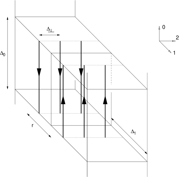
Figure 1: The geometry of slabs and blocks in the $d=3$ case. The thick lines symbolize the Polyakov loops, and $\Delta_{\perp}n_{\perp}=L$.

2.2.2 Higher representations

To incorporate the Polyakov loop correlator in higher representations in the multi-level scheme described above, higher direct products must be computed. We generalize Eq. 7 so that, for any two color tensors $U$ and $V$ of rank $n$ and $m$, (the color indices taking values 1 to $N$),

$$(U\otimes V)_{\alpha_{1},\dots,\alpha_{n};\beta_{1},\dots,\beta_{m}}=U_{\alpha_{1},\dots,\alpha_{n}}V_{\beta_{1},\dots,\beta_{m}}.$$ (16)

With the definition

$${\bf T}^{\uparrow\uparrow}_{s}(x,y)={\bf T}^{\uparrow}_{s}(x)\otimes{\bf T}^{\uparrow}_{s}(y),$$ (17)

we can define the ${\cal N}$-ality 2 version of the two-line operator

$${\bf T}^{\downarrow\downarrow\uparrow\uparrow}_{s}(x,y)={\bf T}^{\uparrow\uparrow}_{s}(x,x)^{*}\otimes{\bf T}^{\uparrow\uparrow}_{s}(y,y),$$ (18)

which has $N^{4}\times N^{4}$ entries. The product of two such objects is defined by the property

$$\left((U\otimes U^{\prime})\otimes(U^{\prime\prime}\otimes U^{\prime\prime\prime})\right)\cdot\left((V\otimes V^{\prime})\otimes(V^{\prime\prime}\otimes V^{\prime\prime\prime})\right)=(UV\otimes U^{\prime}V^{\prime})\otimes(U^{\prime\prime}V^{\prime\prime}\otimes U^{\prime\prime\prime}V^{\prime\prime\prime}).$$

and multilinearity.

The observables needed to compute the correlator in the 2a and 2s representations may now be expressed as

$$P_{\rm F}^{2}(x)^{*}P_{\rm F}^{2}(y) = {\bf Tr}_{\rm 2i}\left\{{\cal T}~{}{\textstyle\prod_{s=0}^{n_{0}-1}}~{}{\bf T}^{\downarrow\downarrow\uparrow\uparrow}_{s}(x,y)\right\},$$ (19)

$${\rm Tr\,}\{U_{P}(x)^{2}\}^{*}{\rm Tr\,}\{U_{P}(y)^{2}\} = {\bf Tr}_{\rm 2ii}\left\{{\cal T}~{}{\textstyle\prod_{s=0}^{n_{0}-1}}~{}{\bf T}^{\downarrow\downarrow\uparrow\uparrow}_{s}(x,y)\right\},$$ (20)

$$P_{\rm F}^{2}(x)^{*}{\rm Tr\,}\{U_{P}(y)^{2}\} = {\bf Tr}_{\rm 2iii}\left\{{\cal T}~{}{\textstyle\prod_{s=0}^{n_{0}-1}}~{}{\bf T}^{\downarrow\downarrow\uparrow\uparrow}_{s}(x,y)\right\},$$ (21)

where the trace operations are defined such that

$${\bf Tr}_{\rm 2i}\{(U\otimes U^{\prime})\otimes(V\otimes V^{\prime})\} = {\rm Tr\,}\{U\}~{}{\rm Tr\,}\{U^{\prime}\}~{}{\rm Tr\,}\{V\}~{}{\rm Tr\,}\{V^{\prime}\},$$ (22)

$${\bf Tr}_{\rm 2ii}\{(U\otimes U^{\prime})\otimes(V\otimes V^{\prime})\} = {\rm Tr\,}\{UU^{\prime}\}~{}{\rm Tr\,}\{VV^{\prime}\},$$ (23)

$${\bf Tr}_{\rm 2iii}\{(U\otimes U^{\prime})\otimes(V\otimes V^{\prime})\} = {\rm Tr\,}\{U\}~{}{\rm Tr\,}\{U^{\prime}\}~{}{\rm Tr\,}\{VV^{\prime}\}.$$ (24)

For the adjoint representation, one needs the definition

$${\bf T}^{\uparrow\downarrow\downarrow\uparrow}_{s}(x,y)={\bf T}^{\downarrow\uparrow}_{s}(x,x)^{*}\otimes{\bf T}^{\downarrow\uparrow}_{s}(y,y).$$ (25)

Then

$$|P_{\rm F}(x)P_{\rm F}(y)|^{2} = {\bf Tr}_{\rm 2i}\left\{{\cal T}~{}{\textstyle\prod_{s=0}^{n_{0}-1}}~{}{\bf T}^{\uparrow\downarrow\downarrow\uparrow}_{s}(x,y)\right\}$$ (26)

$$|P_{\rm F}(x)|^{2} = {\bf Tr}\left\{{\cal T}~{}{\textstyle\prod_{s=0}^{n_{0}-1}}{\bf T}^{\downarrow\uparrow}_{s}(x,x)\right\}$$ (27)

As in going from Eq. 12 to Eq. 13, the expectation values of the correlators can now be written in a form suitable for the implementation of the multi-level algorithm. In the expectation value of the Polyakov loop correlators one may take the average value $\langle.\rangle_{s}$ inside a slab of each two-line operator appearing in Eq. 19—21, 26—27. To exploit the factorization into blocks along the direction $\hat{1}$, we evaluate the slab-averages as in Eq. 14 by taking the block average values of the line operators on the right-hand side of Eq. 18 and Eq. 25.

It should be clear that the Polyakov loop correlator can be obtained in a factorized form for any desired representation. Also, the formulae presented hold for any number of dimensions $d\geq 2$. We now turn to some practical considerations concerning the implementation of the algorithm.

2.2.3 Algorithm implementation and efficiency

1. Produce an independent configuration by doing a sufficient number of hybrid over-relaxation sweeps through the whole lattice; 2. for all slabs, in increasing time order: 3.        repeat the following procedure $m_{s}$ times: 4.              update the slab and then, for all blocks: 5.                    do $m_{b}$ measurements of the needed line operators                    inside the block separated by an update within the block 6.              compute the two-line operators and add them to their slab averages; 7.        multiply the product of previous two-link operators by the new one; 8. compute the traces.

Table 1: Outline of the three-level algorithm.

The three-level algorithm described above that we applied to $d=3$ SU(5) simulations is in essence the Lüscher-Weisz algorithm, where however the slab-averages of the two-line operators are computed in a factorized way. Due to the factorization along the direction $\hat{1}$, we measure the Polyakov loop correlator in that direction only. The additional factorization breaks translational invariance and the symmetry between directions $\hat{1}$ and $\hat{2}$ and thus leads to a loss of statistics; on the other hand the short-distance fluctuations of the one-line operators can be averaged out separately. Test studies [36] in the $d=3$ SU(2) theory show that the three-level algorithm improves on the original Lüscher-Weisz algorithm for $r\geq 0.9$fm, $a=0.08$fm, the latter being superior at shorter distances. This test concerns the static force in the fundamental representation, but in the higher representations, and also at smaller lattice spacing, we expect the additional factorization to pay off already at shorter distances. Since the correlation is obtained at fewer points, but each of them is evaluated more accurately, the memory requirement is lowered.

	$\beta$	$T/a$	$L/a$	$n_{0}$	$n_{1}$	$n_{\perp}$	$n_{\rm meas}$	$r_{0}/a$
$A_{20}$	38	20	22	4	2	11	2536	4.03879(39)
$A_{30}$	38	30	22	6	2	11	2275	4.03943(35)
$B$	44	25	26	5	2	13	1731	4.82879(58)
$C$	54	30	30	5	3	10	1647	6.1323(11)

Table 2: The $d=3$ SU(5) simulation details.

The algorithm proceeds as sketched in Tab. 1 (the scope of loops are given by the indentation of the lines). The simulation parameters are given in Tab. 2. The number $n_{0}$ of slabs and $n_{1}$ of blocks per slab can be found there. Because of memory limitations, we only computed the line-operators every second or third point in the $\hat{2}$ direction. The number $n_{\perp}$ in Tab. 2 is the number of transverse coordinates at which the line-operators were computed. We measured the correlation from distance $2a$ to $10a$ in all simulations; hence $n_{r}=9$. And in all simulations $m_{s}=20$ and $m_{b}=60$ (see Tab. 1 for the meaning of these parameters). We did not use the multihit technique [37], because for the higher representations it increases the number of two-line operator multiplications, which are expensive at large $N$. Finally, the total number of update sweeps between measurements is $60$. They are grouped in compound sweeps consisting of one heat-bath followed by three over-relaxation sweeps [39, 40, 41]. This proved sufficient to decorrelate almost entirely successive measurements of the observables and still represents a negligible overhead with respect to the measurements. To update the slabs we used three compound sweeps, and only one between line-operator measurements inside the blocks.

The program goes from slab to slab in a time-ordered way. It is in order to save memory that each measurement of the two-line operator slab-averages is followed by their multiplication with the product of the preceding slab-averages. In this way, the program only needs enough memory for two fields of the size

$$n_{1}\times n_{\perp}\times n_{r}\times{\rm size}({\bf T}).$$

The two-line operator (18) contains $N^{8}$ complex numbers. Hence we reach the requirement $\sim 4\cdot 10^{8}$ 32-bit floating numbers for simulation C.

For a given separation $r$, we correlate the line operators as far as possible from the boundaries. That is, for the correlator at a separation of $2na$, we correlate the line operators computed at $x_{1}=\Delta_{1}-na$ with those computed at $x_{1}=\Delta_{1}+na$ (and all equivalent points by translation of distance $\Delta_{1}$ in the direction $\hat{1}$). For a separation of $(2n+1)a$, we average the correlation obtained at $(\Delta_{1}-na,\Delta_{1}+(n+1)a)$ with that obtained at $(\Delta_{1}-(n+1)a,\Delta_{1}+na)$.

We introduce the notation

$$\Gamma_{\rm R}(r)=\langle P_{\rm R}^{*}(x)P_{\rm R}(x+r\hat{1})\rangle$$ (28)

for the on-axis Polyakov loop correlator. Tab. 3 gives these correlators in the fundamental, as well as in the ${\cal N}$-ality 2 representations 2a and 2s in simulation B. It turns out that these measurements in the different representations are quite strongly correlated at short distances (and essentially uncorrelated beyond $r=r_{0}$), so that it will be advantageous to take the ratio of static forces measured in the same simulation. With the tuning of the algorithm used, we are able to maintain a signal to noise ratio below $1\%$ beyond 1fm in the fundamental representation and beyond 0.7fm in the 2a representation. The performance (and memory requirements) of the algorithm behave favourably if the time extent is increased, as a comparison of the data from simulations $A_{20}$ and $A_{30}$ will reveal.

To give an idea of the computing effort involved, one full measurement in simulation $B$ took 1.7 hour on a single 2.4GHz Opteron with 4GB of memory, while the 60 full-lattice sweeps between each of these full measurements took 61 seconds.

The statistical errors are estimated with the Gamma method [42]. Simulation $C$ was run with 8 replica (= independent simulations) and the others with 4 replica; we checked in all cases that the results are consistent across replica. We also found that using the jacknife method gave error estimates in agreement with the Gamma method, which is hardly surprising since the successive measurements were very decorrelated in these runs.

3 The static force in the fundamental representation

In this section we present our data on the static force. It is found that the quantity $r_{0}^{2}\sigma$ has very small discretization errors. By comparison with the SU(3) data of Lüscher and Weisz [10] and the SU(2) data of Majumdar [31] (see also [33]), we find that it is also very weakly dependent on the number of colors $N$. We then compare the $N=2,3,5$ results for the effective central charge at fixed value of $r_{0}$.

3.1 The SU(5) static force

The static force is defined at finite lattice spacing by

$$F_{\rm R}(\bar{r})=\textstyle{\frac{1}{a}}[V_{\rm R}(r+a)-V_{\rm R}(r)],\qquad V_{\rm R}(r)=-\frac{1}{T}\log\Gamma_{\rm R}(r).$$ (29)

We reuse the tree-level improved argument $\bar{r}=r+a/2+{\rm O}(a^{2})$ of the function $F_{\rm R}$ given in [10]. The fundamental static force obtained in simulation B can be found in Tab. 4. The reference scale $r_{0}/a$ given in Tab. 2 is obtained in the standard manner [15], by linearly interpolating $(r/a)^{2}$ as a function of $r^{2}F(r)$ to the abscissa 1.65.

To a first approximation, the force is constant beyond 0.75fm, signalling linear confinement. To investigate this in more detail, we find it useful to define the quantity

$$\sigma(r)=F(r)-\frac{\pi}{24r^{2}}.$$ (30)

If the Lüscher term does provide the leading asymptotic correction to the linear potential [9], then this quantity deserves the name of effective string tension and the notation is appropriate. Note that by definition,

$$r_{0}^{2}\sigma(r_{0})=1.65-{\textstyle\frac{\pi}{24}}=1.519100\dots$$ (31)

at all lattice spacings. In particular, discretization errors on $r_{0}^{2}\sigma(r)$ are automatically reduced around separation $r=r_{0}$.

The function $r_{0}^{2}\sigma(r)$ is plotted in Fig. 2 for all data sets. The practical advantage of considering this function is that it is very flat beyond 0.4fm (note the scale of the vertical axis); in this way, the data can be visualized in more detail. We firstly remark that the data $A_{20}$ and $A_{30}$ agree within error bars at all separations; the common abscissa of these data points have been split symmetrically for better visibility. This indicates that the time extent $T\approx 5r_{0}$ is sufficient to ‘filter out’ the ground state of the transfer matrix in the presence of the two Polyakov loops [10] separated by $r\leq 2r_{0}$; the statement holds of course at the precision to which we have been able to compute the static force.

Secondly, the scaling violations of $r_{0}^{2}\sigma(r)$ are at the few permille level (or less) around $r=1.4r_{0}$. To carry out a continuum extrapolation, we need to interpolate $r_{0}^{2}F(xr_{0})$ to a few fixed values of $x$. This is done by a linear interpolation in $1/x^{2}$ (in [10] a three-point interpolation in $1/x^{2}$ was used). The result is given for each simulation in Tab. 6. It turns out that extrapolating these quantities to the continuum with the expected ${\rm O}(a^{2})$ corrections [43] yields poor $\chi^{2}$ values (see Fig. 8). Therefore we extrapolate the data from the two smaller lattice spacings linearly in $(a/r_{0})^{2}$, and use a quadratic fit to all three lattice spacings to estimate the uncertainty associated with the linear fit; we refer the reader to the appendix for more details. At least one additional simulation at a lattice spacing of $a\approx 0.1r_{0}$ is required to take the continuum limit in a way that does not blow up the final uncertainty.

Finally, we did not investigate finite-volume effects, but since $2.45{\rm fm}<L<2.72{\rm fm}$ in these simulations, we do not expect them to affect our conclusions.

3.2 The quantity $\sigma r_{0}^{2}$ for all $N$

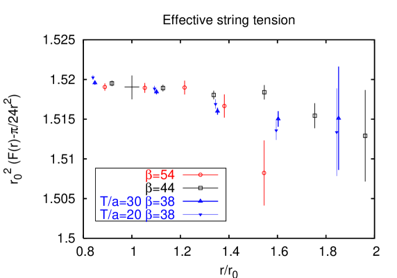
Figure 2: The SU(5) effective string tension in units of $r_{0}^{-2}$. By interpolation all data go through the cross (by definition of $r_{0}$).

In comparing SU($N$) gauge theories, perhaps the most natural way to set the common energy scale is by equating their (fundamental) string tensions $\sigma$. This quantity is however more difficult to compute with high precision than $r_{0}$, because it involves an extrapolation to infinite string length [15]. For that reason, we are now going to show that the dimensionless quantity $r_{0}^{2}\sigma$ is $N$-independent to a precision better than $1\%$. As a consequence, comparing SU($N$) gauge theories at fixed value of $r_{0}$ is essentially equivalent to fixing the value of $\sigma$.

We can extract the effective string tension at 1fm straightforwardly. A direct comparison of our data with the SU(3) data of Lüscher and Weisz at the same lattice spacing $a=0.207r_{0}$ gives

$$r_{0}^{2}\sigma(2r_{0}) = 1.5124(65),\qquad{\rm SU}(5),~{}\beta=44,$$ (32)

$$r_{0}^{2}\sigma(2r_{0}) = 1.51776(24),\qquad{\rm SU}(3),~{}\beta=15.$$ (33)

Interestingly, the string tension has also been computed in the closed string channel by Teper [4] at these values of $\beta$. Using the values of $r_{0}$ quoted above, we have

$${\rm SU}(5): r_{0}^{2}~{}\sigma_{\rm closed}=1.521(8)$$ (34)

$${\rm SU}(3): r_{0}^{2}~{}\sigma_{\rm closed}=1.520(14).$$ (35)

The string tension quoted by Teper is also an effective string tension (as defined by $m(L)=\sigma(L)L-{\textstyle\frac{\pi}{6L}}$), but at a closed string length of $3.3r_{0}$, where higher order string corrections are presumably much reduced. In the SU(3) case an additional calculation of his at string length of $5.0r_{0}$ yielded the same string tension (and accuracy). We conclude that the closed string tension extracted from torelon masses agrees with the open string tension extracted from the static force at 1fm at a precision of $1\%$.

Majumdar [31] reports almost identical values of $r_{0}^{2}\sigma$ in the SU(2) theory at lattice spacings $a\leq 0.16r_{0}$. In particular, a comparison between SU(2) and SU(3) closer to the continuum yields

$$r_{0}^{2}\sigma(2r_{0}) = 1.523(2)\quad\qquad{\rm SU}(2),~{}\beta=7.5,~{}r_{0}=6.29a$$ (36)

$$r_{0}^{2}\sigma(2r_{0}) = 1.51999(34)\qquad{\rm SU}(3),~{}\beta=20,~{}r_{0}=6.71a.$$ (37)

Cutoff effects on $r_{0}^{2}\sigma$ are thus seen to lie well below the percent level. Assuming that no strong $N$-dependence appears beyond $N=5$ (the contrary would be very surprising in view of the results obtained in [4]), we reach the following remarkable conclusion:

$$r_{0}^{2}\sigma=1.52\cdot(1\pm 1\%)\qquad\qquad\forall N\geq 2,\quad a\leq 0.21r_{0}.$$ (38)

In particular,

$$\sigma=\sigma(r_{0})\cdot(1\pm 1\%)\qquad\qquad\forall N\geq 2$$ (39)

holds in the continuum limit (see also Fig. 8).

3.3 The effective central charge

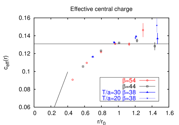
Figure 3: The SU(5) effective central charge at several lattice spacings. The perturbative prediction is shown at short distance, and the horizontal line marks the value ${\textstyle\frac{\pi}{24}}$.

The effective central charge is defined by

$$c(\tilde{r})=-{\textstyle\frac{1}{2}}\tilde{r}^{3}[V(r-a)-2V(r)+V(r+a)]/a^{2},$$ (40)

where $\tilde{r}=r+{\rm O}(a^{2})$ is defined in [10]. Fig. 3 shows the computed effective central charge $c(r)$ in the range of distances 0.25 to 0.75fm. A precocious convergence to values within $5\%$ of ${\textstyle\frac{\pi}{24}}$ is observed.

By eye, the data at $\beta=44$ and $\beta=54$ practically fall on top of each other up to 0.6fm, indicating that discretization errors are reasonably small. Beyond that point, the $\beta=54$ data’s accuracy no longer allows for a useful comparison. The data points obtained at the coarsest lattice spacing systematically lie slightly above the other points. This effect was already seen in SU(2) and SU(3) calculations. Also, the data sets $A_{20}$ and $A_{30}$ are well compatible, indicating that the time extent was chosen long enough for the present statistical accuracy.

The expected behaviour at short distances, as given by two-loop perturbation theory [29], is shown on the figure, as well as the universal value ${\textstyle\frac{\pi}{24}}$ expected at long distances. The continuum value of $g^{2}r_{0}$, which determines the slope of the short-distance prediction, was estimated by extrapolating the value of $g_{\rm o}^{2}r_{0}$ of simulations $B$ and $C$ linearly in $g_{\rm o}^{2}a$. Using the continuum value of $\sqrt{\sigma}/g^{2}$ of [4] and Eq. 38 yields a slope smaller by $2\%$; the difference would hardly be noticeable on Fig. 3.

In view of taking the continuum limit, we interpolate $c(xr_{0})$ to a handful of values of $x$. We use a three-point polynomial interpolation in $1/x$ (following [10]); the result is given in Tab. 7. The continuum limit is described in the appendix, where also an alternative definition of the effective central charge is proposed and shown to lead to the same continuum results (Fig. 8).

3.4 The effective central charge for all $N$

Figure 4: The effective central charge for several gauge groups. The SU(3) data is taken from [10], the SU(2) data from [32]. The perturbative prediction is shown at short distance (the slope increases slightly with $N$) and the Nambu-Goto prediction at long distances, while the horizontal line marks the value ${\textstyle\frac{\pi}{24}}$.

It is now interesting to compare the effective central charge curves obtained for $N=2,3$ and 5. If we attempted to compare the data in the continuum limit, the continuum extrapolation would lead to the dominant source of uncertainty, because only three lattice spacings are available at each $N$. Also, the data at the coarsest lattice spacing in the SU(3) and SU(5) data sets are not (always) consistent with O($a^{2}$) corrections. For that reason we prefer to compare the data sets at the smallest common lattice spacing. This corresponds to $\beta=7.5,~{}20$ and 54 for $N=2,3$ and 5 respectively. The values of $r_{0}/a$, 6.29, 6.71 and 6.13 respectively, indeed are matched at the $10\%$ level.

The comparison is illustrated on Fig. 4. At short distances, the curves are expected to differ by O($1/N^{2}$) from perturbation theory and the scaling of $g^{2}Nr_{0}$. This is indicated by the straight solid lines which stop short at $0.4r_{0}$ around where perturbation theory ceases to be accurate. Remarkably, all three curves seem to approach the value of ${\textstyle\frac{\pi}{24}}$ at larger distances. This fact constitutes strong evidence for the universality of the string correction in $d=3$ SU($N$) gauge theories. On the other hand, the approach to the asymptotic value is surprisingly precocious. The numerical closeness of $c(r)$ to ${\textstyle\frac{\pi}{24}}$ is probably deceptive, in so far that it suggests that any higher order string corrections are already very small below 1fm. The leading correction term is O($1/\sigma r^{2}$), and its coefficient is universal and positive in the effective theory describing the massless transverse fluctuations of the flux-tube [10]. The Nambu-Goto string in a non-critical number of dimensions corresponds to a special case in this class of theories; it provides a consistent analytic prediction for the $r\times T$ Polyakov loop correlator to any finite order in $1/r$ or $1/T$ [10]. It predicts an effective central charge [44] of the form

$$c^{\rm(NG)}(r)=\frac{\pi}{24}~{}\left(1-{\textstyle\frac{\pi}{12\sigma r^{2}}}\right)^{-3/2},$$ (41)

shown for illustration in the upper right corner of Fig. 4. It suggests that the effective string theory becomes accurate at significantly larger distances. To summarize, since $c(r)<{\textstyle\frac{\pi}{24}}$ at short distances; since the $1/r$ series for $c(r)$ at large distances is almost certainly asymptotic; and since the O($1/\sigma r^{2}$) term is positive, this term improves on the leading order prediction at the earliest when the effective central charge computed in the gauge theory rises above the value ${\textstyle\frac{\pi}{24}}$.

The preceding arguments thus motivate the definition of the distance $r_{\rm s}$ where the effective central charge crosses ${\textstyle\frac{\pi}{24}}$:

$$c(r_{\rm s})\equiv{\textstyle\frac{\pi}{24}}.$$ (42)

This distance is a natural separation scale between the perturbative regime and the string regime. The ratio $r_{\rm s}/r_{0}$ is expected to have a continuum limit with O($a^{2}$) discretization errors, and at finite lattice spacing an interpolation formula must be prescribed to define it. In general we propose to use a three-point polynomial interpolation in $r$ using the three nearest data points, because $c(r)$ has quite some curvature around $r_{\rm s}$.

Figure 5: The dependence of $r_{\rm s}/r_{0}$ on the number of colors $N$. The SU(3) data is taken from [10], the SU(2) data from [32].

Fig. 4 shows quite strikingly that as the number of colors is increased, the curve $c(r)$ interpolates over an even shorter distance range between the perturbative behaviour and the value ${\textstyle\frac{\pi}{24}}$. We therefore study the $N$-dependence of $r_{\rm s}/r_{0}$. To do so we shall presently use a simple linear interpolation between the two nearest points to the crossing, because the SU(2) and SU(5) data rapidly become less accurate beyond the crossing. Luckily in all three cases there is a point lying almost exactly at ${\textstyle\frac{\pi}{24}}$, which makes the details of the interpolation a negligible source of uncertainty. In order to have the same discretization scheme for all data sets, we replaced $r$ by $\tilde{r}$ in the SU(2) values of the effective central charge [31, 32]. We thus find:

$$\frac{r_{\rm s}}{r_{0}}=\left\{\begin{array}[]{l@{\quad}l}1.79(5)&N=2\\ 1.32(5)&N=3\\ 0.96(2)&N=5\\ \end{array}\right.$$ (43)

The smaller uncertainty at SU(5) reflects the fact that $c(r)$ cuts the horizontal ${\textstyle\frac{\pi}{24}}$ line at a shorter distance and with a larger slope than for SU(2) and SU(3). At $N=5,~{}\beta=44$ we obtain $r_{\rm s}/r_{0}=0.977(11)$, in agreement with (43). The trend that $r_{\rm s}/r_{0}$ strongly decreases with the number of colors is quite striking and constitutes a rare example of a physical quantity in SU($N$) gauge theories which has a strong $N$-dependence. This dependence is shown on Fig. 5. The data is well compatible with a linear function in $1/N$:

$$\frac{r_{\rm s}}{r_{0}}=0.402(45)+2.80(20)\frac{1}{N}\qquad(\chi^{2}/{\rm d.o.f}\simeq 0.01).$$ (44)

Could it be that $r_{\rm s}$ becomes as small as 0.2fm in the large-$N$ limit? An SU(8) calculation would provide a useful clue to answer the question. In the mean time, we can compare the value to two other distance scales which are natural in this context. The first comes from the Arvis formula, Eq. 41. The latter becomes singular at a distance $r_{a}$ given by

$$\frac{r_{a}}{r_{0}}=\sqrt{\frac{\pi}{12\sigma}}~{}\frac{1}{r_{0}}=0.415(4).$$ (45)

where we have used Eq. 38. It is intriguing that the naively obtained value $r_{\rm s}(N=\infty)$ is compatible with $r_{a}$. Secondly, the dotted line on Fig. 4 is the continuation of the curve corresponding to the perturbative two-loop result [29] in the large-$N$ limit (using $\lim_{N\to\infty}\sqrt{\sigma}/g^{2}N=0.1975(10)$ from [4] and Eq. 38). It cuts ${\textstyle\frac{\pi}{24}}$ at distance $r_{\rm pt}$ given by

$$\frac{r_{\rm pt}}{r_{0}}=0.527(4).$$ (46)

The rise of $c(r)$ up to and beyond ${\textstyle\frac{\pi}{24}}$, which becomes more rapid as $N$ is increased, could be a sign that the asymptotic series in $(\sigma r^{2})^{-1}$ provided by the effective string theory converges better at a given value of $\sqrt{\sigma}r$ if the number of colors is increased. This is not unconceivable, because certain effects such as the radiation of glueballs by a highly excited string, which exist in the gauge theory but are neglected in the effective string theory, are $1/N^{2}$ suppressed.

4 What is the size of Casimir scaling violations?

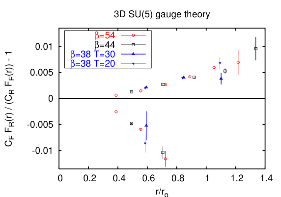
Figure 6: Relative deviation of the force ratios $F_{\rm R}/F_{\rm F}$ from Casimir scaling in the SU(5) gauge theory. The points above and below zero correspond to the representations R=2a and R=2s respectively.

We now address this question in the case of the two smallest irreducible representations of SU(5) of ${\cal N}$-ality 2. These are obtained by taking the direct product of two fundamental charges and forming the (anti)symmetric linear combinations, as in Eq. 5 and 6. We discuss the ratio of these forces to the force in the fundamental representation. Note that, unlike the ratio of static potentials, this quantity has a continuum limit.

The Casimir scaling prediction is, in a range of distances $r_{\rm min}<r<r_{\rm max}$,

$$\frac{F_{\rm 2a}(r)}{F_{1}(r)} \stackrel{{\scriptstyle\rm CS}}{{=}} \frac{C_{\rm 2a}}{C_{1}}=\left.\frac{2(N-2)}{N-1}\right|_{N=5}=\frac{3}{2}.$$ (47)

$$\frac{F_{\rm 2s}(r)}{F_{1}(r)} \stackrel{{\scriptstyle\rm CS}}{{=}} \frac{C_{\rm 2s}}{C_{1}}=\left.\frac{2(N+2)}{N+1}\right|_{N=5}=\frac{7}{3}.$$ (48)

Perturbation theory predicts [29]

$$F_{\rm R}(r)=\frac{C_{\rm R}g^{2}}{2\pi r}\left[1+\textstyle{\frac{7}{32}}g^{2}Nr+O((g^{2}Nr)^{2})\right].$$ (49)

In particular, Casimir scaling of static forces holds at least to order $g^{4}$.

The result for the ratio of static forces obtained in simulation $B$ is given in Tab. 4. Fig. 6 shows the Monte-Carlo data on the relative deviations of $F_{\rm 2a}/F_{1}$ from Casimir scaling in the SU(5) lattice gauge theory. The window in $r$ is 0.2—0.7fm. Notice the scale of the vertical axis: the (2a) data points indicate a positive relative deviation which grows from about 0.001 to 0.01 in that range of distances. The (2s) data on the other hand shows a stronger, negative deviation. This is expected, since the static charges in this representation can be screened to (2a). The force between charges in the adjoint representation, which can be screened completely, also exhibits this behaviour [25]. A positive deviation is thus rather special. It will remain positive at larger distances if the $k=2$ string tension is larger than $C_{\rm 2a}/C_{1}\cdot\sigma$, or if it is given exactly by that expression and its central charge by ${\textstyle\frac{\pi}{24}}$.

Beyond $r_{0}$, we are perhaps seeing the effects of finite time extent: there is a 1.9$\sigma$ discrepancy between the third (2a) data points of simulations $A_{20}$ and $A_{30}$ on Fig. 6. If present, this effect comes from $F_{\rm 2a}$, because the quantity $r_{0}^{2}F_{1}(r)$ is perfectly consistent between $A_{20}$ and $A_{30}$ (see Tab. 6).

It is clear from Fig. 6 that the (absolute) discretization errors are bounded by 0.001. The force ratio $F_{\rm 2a}/F_{1}$ at distance $xr_{0}$ has been interpolated to a few values of $x$ in Tab. 10. The two-parameter function $f(x)=px^{2}/(x^{2}+q^{2})$ was used to interpolate the quantity plotted on Fig. 6, but the result never actually differs by more than one standard deviation from a simple linear interpolation in $x$. Tab. 10 also gives the result of a continuum extrapolation performed along the same lines as for $r_{0}^{2}F_{1}(r)$.

Figure 7: The SU(5) effective central charge in the 2a representation. The perturbative prediction is shown at short distance and the Nambu-Goto prediction at long distance. The horizontal line marks the value ${\textstyle\frac{\pi}{24}}$.

Since there is a stable string in the ${\cal N}$-ality 2 sector, it makes sense to consider the effective central charge in the 2a representation; Fig. 7 shows our data on $c_{\rm 2a}(r)$. At short distances, it is roughly a factor 3/2 larger than in the fundamental representation, as predicted by perturbation theory. The curve seems to flatten off, as it does in the fundamental representation, but the data does not extend far enough to show whether it will bend down towards ${\textstyle\frac{\pi}{24}}$, as we expect it to [45]. It was observed [30] in closed $k=2$ SU(8) strings that $c_{\rm 2a}<\frac{\sigma_{\rm 2a}}{\sigma_{1}}c_{1}$.

4.1 Mixed representation correlators

It is interesting to look at the cross correlation $\langle P_{\rm 2a}(x)^{*}P_{\rm 2s}(x+r\hat{1})\rangle$. There is no symmetry which makes this correlator vanish. However we find that it is consistent with zero. For instance, the ‘overlap’

$$\frac{\langle P_{\rm 2a}(x)^{*}P_{\rm 2s}(x+r\hat{1})\rangle}{\sqrt{\Gamma_{\rm 2a}(r)\Gamma_{\rm 2s}(r)}}$$

is consistent with zero in simulation $B$ with a statistical uncertainty of $5\cdot 10^{-5}$, $3\cdot 10^{-4}$ and $4\cdot 10^{-3}$ at distances $r=2a,~{}3a$ and $4a$ respectively. Since

$$\langle P_{\rm 2a}(x)^{*}P_{\rm 2s}(y)\rangle={\textstyle\frac{1}{4}}\left(\langle({\rm Tr\,}\{U_{P}^{*}\})^{2}(x)~{}({\rm Tr\,}\{U_{P}\})^{2}(y)\rangle-\langle{\rm Tr\,}\{U_{P}^{2}\}^{*}(x)~{}{\rm Tr\,}\{U_{P}^{2}\}(y)\rangle\right),$$

the statement that the cross correlation vanishes is equivalent to the property that the two correlators on the RHS of this equation are equal.

The interpretation that we propose is based on the observation that the direct product of the representations $({\rm 2a})^{*}$ and 2s does not contain the singlet representation (though it does contain the adjoint representation). Therefore if we imagine inserting the static particles adiabatically into the system, they initially have an overall color charge. The only way the free energy can be made finite is if virtual adjoint charges screen the system. Since the external color charge object is extended, it presumably costs a large amount of energy to screen it. In addition, statistically speaking the color of the virtual adjoint charge must match that of the static system, which happens with a probability of order $1/N^{2}$. Thus one expects the overlap to be $1/N^{2}$ color-phase-space suppressed [28]. All this results in a very small cross-correlation of the Polyakov loops. This large-$N$ argument was already made in [30] to explain the fact that in closed $k$-string computations [28, 30], the wavefunction of the lightest state is very well approximated by a (fuzzy) Polyakov loop in the totally antisymmetric representation of ${\cal N}$-ality $k$.

5 Conclusion

We computed the static force in the $d=3$ SU(5) gauge theory employing an efficient three-level algorithm. Linear confinement is observed, and the effective string tension defined in Eq. 30 is essentially constant beyond 0.5fm. The string tension extracted at 1fm agrees with the closed string tension extracted from torelon spectroscopy [4].

By comparison with existing SU(2) [31, 33] and SU(3) [10] data, the quantity $\sigma r_{0}^{2}$ is found to be independent of the number of colors at the $1\%$ level; it also has very small discretization errors. Thus comparing SU($N$) gauge theories at common string tension or common Sommer reference scale is equivalent at that level of precision.

The effective central charge $c(r)$ was obtained in the range 0.25—0.75fm. It converges to within $5\%$ of the expected asymptotic value of ${\textstyle\frac{\pi}{24}}$, confirming the multiplicity and the bosonic nature of the flux-tube’s massless degrees of freedom. A comparison with the SU(2) and SU(3) data reveals that the distance $r_{\rm s}$ where $c(r)$ crosses the value ${\textstyle\frac{\pi}{24}}$ decreases steadily by almost a factor two from SU(2) to SU(5). Since (bosonic) effective string theory predicts that the asymptotic value is approached from above [3], it is tempting to speculate that the asymptotic expansion’s accuracy is higher at a fixed value of $\sqrt{\sigma}r$ for larger $N$.

We also studied the static force in the symmetrized (2s) and antisymmetrized (2a) direct product representations of two ‘quarks’. For $N\geq 4$, it is known [28] that such static charges of ${\cal N}$-ality 2 are linearly confined with a different string tension from the fundamental one. And indeed we find that the ratio $F_{\rm 2a}/F_{1}$ is constant to a first approximation, confirming the linear confinement property. Furthermore, it is very close to the Casimir scaling prediction (3/2 in this case). A more detailed study reveals that deviations are present at the $0.1\%$ to $1\%$ level in the range 0.2—0.7fm. They are positive, unlike the case of the adjoint static force [25] where screening of the adjoint flux must set in at some distance $r$. The 2s representation on the other hand exhibits a negative deviation, as one expects if there is a single stable string per ${\cal N}$-ality and screening occurs.

Since the representation 2a has ${\cal N}$-ality 2 and has the smallest quadratic Casimir of all irreducible representations in that sector, one might expect to find again a precocious onset of the effective central charge $c_{\rm 2a}(r)$ for the $k=2$ string. This is not the case: at $r=r_{0}$, where $c(r)$ lies within a few percent of ${\textstyle\frac{\pi}{24}}$, $c_{\rm 2a}(r)$ is almost as large as $\frac{3}{2}\cdot{\textstyle\frac{\pi}{24}}$. Data at further distances is needed to see whether it decreases towards ${\textstyle\frac{\pi}{24}}$.

Acknowledgements

I thank the computer team of DESY/NIC for providing an efficient batch system. I am indebted to Pushan Majumdar for communicating unpublished SU(2) data and reading the manuscript. I also thank York Schröder for discussions and Rainer Sommer for a critical reading of the manuscript.

Appendix: discretization errors and the continuum limit

The quantity $r_{0}^{2}F(r)$ has been extrapolated linearly in $(a/r_{0})^{2}$ to the continuum, using the data from simulations $B$ and $C$. This is our best estimate in the continuum limit and it can be found in Tab. 6. The first number in brackets is the statistical error on the result (there is no $\chi^{2}$). To estimate the systematic uncertainty on this procedure, we also do a quadratic fit in $(a/r_{0})^{2}$ to simulations $A_{30}$, $B$ and $C$ (again, there is no $\chi^{2}$). The second number given in brackets is the continuum value obtained by quadratic extrapolation minus the quoted continuum result. Thus a conservative error estimate is the maximum of the absolute value of the two numbers in brackets. The continuum limit is illustrated for $r_{0}^{2}\sigma(r)$, which is equivalent to $r_{0}^{2}F(r)$ for this purpose, on Fig. 8.

We proceeded in the same way for $F_{2a}(r)/F_{1}(r)$ (Tab. 10). For the effective central charge, we also give the continuum $c(r)$ obtained in this way in Tab. 7. Recall that the definition of Ref. [10] was used to define $c(r)$ at finite lattice spacing. We now show that a different definition gives the same result in the continuum limit.

We propose to determine the parameters $a^{2}\tilde{\sigma}(r),~{}a\tilde{\mu}(r)$ and $\tilde{c}(r)$ by

$$\tilde{c}(r) = -\frac{r(r-a)(r+a)}{2a^{2}}~{}\left(V(r-a)-2V(r)+V(r+a)\right)$$ (50)

$$a^{2}\tilde{\sigma}(r) = {\textstyle\frac{1}{2}}(r-a)~{}V(r-a)-r~{}V(r)+{\textstyle\frac{1}{2}}(r+a)~{}V(r+a)$$ (51)

$$a\tilde{\mu}(r) = -\frac{(r-a)(r+\frac{a}{2})}{a}~{}V(r-a)+\frac{2r^{2}}{a}~{}V(r)-\frac{(r+a)(r-\frac{a}{2})}{a}~{}V(r+a).$$ (52)

This new definition is such that if the on-axis lattice Polyakov loop correlator was given by

$$e^{-V_{0}(r)T},\qquad V_{0}(r)=\mu+\sigma r-\frac{c}{r},$$ (53)

then the effective parameters match those appearing in $V_{0}(r)$ exactly. Note that the functions $c$ and $\tilde{c}$ differ only by O($a^{2}$) terms, and that $\tilde{c}(r)$ is simply a factor $(1-(a/r)^{2})$ times the ‘naive’ definition of the effective central charge used in [31]. And indeed, comparing Tab. 8 to Tab. 7, we find that $\tilde{c}(r)$ is compatible with $c(r)$ in the continuum limit, as it should be; see Fig. 8 for an illustration. This consistency-check is also a test of our error analysis.

Figure 8: Continuum extrapolation of the effective string tension $r_{0}^{2}\sigma(r)=r_{0}^{2}F(r)-{\textstyle\frac{\pi}{24}}(r_{0}/r)^{2}$ and two definitions of the central charge $c(r)$ and $\tilde{c}(r)$ in $d=3$ SU(5) gauge theory. The result, with its final error bar, is shown at vanishing abscissa.

$r/a$	$\Gamma_{1}(r)$	$\Gamma_{2a}(r)$	$\Gamma_{2s}(r)$
2	$7.4136(20)\cdot 10^{-4}$	$2.00130(80)\cdot 10^{-5}$	$5.1040(32)\cdot 10^{-8}$
3	$8.6971(40)\cdot 10^{-5}$	$8.0083(57)\cdot 10^{-7}$	$3.5219(40)\cdot 10^{-10}$
4	$1.29486(95)\cdot 10^{-5}$	$4.5651(52)\cdot 10^{-8}$	$4.332(24)\cdot 10^{-12}$
5	$2.1498(22)\cdot 10^{-6}$	$3.0544(48)\cdot 10^{-8}$	$5.41(93)\cdot 10^{-14}$
6	$3.7784(53)\cdot 10^{-7}$	$2.2198(54)\cdot 10^{-10}$	–
7	$6.862(12)\cdot 10^{-8}$	$1.676(10)\cdot 10^{-11}$	–
8	$1.2705(31)\cdot 10^{-8}$	$1.317(74)\cdot 10^{-12}$	–
9	$2.3909(81)\cdot 10^{-9}$	$1.36(38)\cdot 10^{-13}$	–
10	$4.553(37)\cdot 10^{-10}$	–	–

Table 3: The raw data of simulation B.

$\bar{r}/a$	$a^{2}F_{1}(\bar{r})$	$F_{2a}(\bar{r})/F_{1}(\bar{r})$	$F_{2s}(\bar{r})/F_{1}(\bar{r})$
2.379	0.0857165(97)	1.501928(46)	2.32216(20)
3.407	0.076183(12)	1.504059(99)	2.3092(28)
4.432	0.071825(15)	1.50613(20)	2.424(95)
5.448	0.069546(18)	1.50793(71)	–
6.458	0.068237(23)	1.5144(33)	–
7.464	0.067463(39)	1.507(33)	–
8.469	0.066812(67)	–	–
9.473	0.06634(25)	–	–

Table 4: The static forces in simulation B.

$\tilde{r}/a$	$c_{1}(\tilde{r})$	$c_{2a}(\tilde{r})$	$c_{2s}(\tilde{r})$
2.808	0.105535(54)	0.15671(10)	0.2560(23)
3.838	0.12320(31)	0.18110(61)	–
4.875	0.13202(48)	0.1916(28)	–
5.902	0.1346(21)	0.158(24)	–
6.920	0.1283(45)	–	–
7.932	0.162(16)	–	–

Table 5: The effective central charges in simulation B.

$r/r_{0}$	$A_{20}$	$A_{30}$	$B$	$C$	cont.
0.50	–	–	1.98604(28)	1.97861(46)	—
0.65	1.81564(22)	1.81552(18)	1.81409(28)	1.81380(35)	1.8133(10)(20)
0.80	1.72229(22)	1.72211(18)	1.72119(15)	1.72108(30)	1.7209(8)(14)
0.95	1.664406(60)	1.664354(48)	1.664300(52)	1.66417(12)	1.6640(3)(-2)
1.00	1.65	1.65	1.65	1.65	1.65
1.05	1.637603(52)	1.637647(41)	1.637694(45)	1.63780(10)	1.6380(3)(1)
1.20	1.60865(24)	1.60849(16)	1.60934(19)	1.61001(44)	1.6111(12)(-2)
1.35	1.58855(46)	1.58815(30)	1.58977(47)	1.5890(11)	1.5877(29)(-45)
1.50	1.57272(81)	1.57386(65)	1.57638(76)	1.5686(32)	1.556(9)(-20)
1.65	1.5615(18)	1.5635(19)	1.5647(10)	–	–
1.80	1.5536(47)	1.5558(55)	1.5551(23)	–	–
2.00	1.562(13)	1.548(32)	1.5451(65)	–	–

Table 6: The quantity $r_{0}^{2}F(r)$ interpolated, and its continuum limit (details in the App.).

$r/r_{0}$	$A_{20}$	$A_{30}$	$B$	$C$	cont.
0.458	–	–	–	0.090714(40)	–
0.65	0.11028(74)	0.11141(56)	0.11284(27)	0.11163(19)	0.1096(7)(-50)
0.80	0.12573(64)	0.12484(50)	0.12348(31)	0.12202(28)	0.1196(9)(-5)
0.95	0.13282(56)	0.13235(44)	0.13006(36)	0.1304(10)	0.131(3)(5)
1.00	0.13424(57)	0.13412(42)	0.13172(46)	0.1314(11)	0.131(3)(4)
1.05	0.13534(71)	0.13564(48)	0.13279(44)	0.1315(12)	0.129(3)(2)
1.20	0.1374(15)	0.1390(10)	0.1344(19)	0.1362(31)	0.139(8)(12)

Table 7: The effective central charge $c(r)$ interpolated, and its continuum limit.

$r/r_{0}$	$A_{20}$	$A_{30}$	$B$	$C$	cont.
0.458	–	–	–	0.098331(44)	–
0.65	0.1105(19)	0.1135(15)	0.11787(15)	0.11611(21)	0.1132(6)(-114)
0.80	0.13196(48)	0.13130(37)	0.12939(35)	0.12533(27)	0.1187(9)(-48)
0.95	0.13995(64)	0.13921(51)	0.13491(33)	0.13260(92)	0.129(2)(3)
1.00	0.14117(58)	0.14074(46)	0.13606(42)	0.1340(11)	0.131(3)(4)
1.05	0.14194(62)	0.14190(45)	0.13690(45)	0.1339(12)	0.1289(32)(7)
1.20	0.1425(14)	0.14393(92)	0.1375(16)	0.1367(27)	0.135(7)(6)

Table 8: The effective central charge $\tilde{c}(r)$ interpolated, and its continuum limit.

$r/r_{0}$	$B$	$C$
0.458	–	0.135447(60)
0.65	0.16725(88)	0.16486(32)
0.80	0.18146(60)	0.17752(69)
0.95	0.1894(20)	0.1849(30)
1.00	0.1912(27)	0.1860(54)
1.05	0.1868(38)	0.186(12)
1.20	0.162(21)	0.135(54)

Table 9: The quantity $c_{\rm 2a}(r)$ interpolated.

$r/r_{0}$	$A_{20}$	$A_{30}$	$B$	$C$	cont.
0.50	–	–	1.324(31)	1.130(39)	–
0.65	2.434(65)	2.567(50)	2.279(50)	2.087(48)	1.77(15)(13)
0.80	3.59(15)	3.693(97)	3.317(66)	3.32(12)	3.3(3)(7)
0.95	5.09(36)	4.01(61)	4.28(15)	4.80(21)	5.7(6)(6)
1.00	5.66(67)	3.94(81)	4.57(21)	5.35(29)	6.6(8)(4)
1.05	6.25(84)	3.87(97)	4.86(30)	5.92(43)	–
1.20	–	8.5(3.2)	6.57(59)	7.0(2.2)	–

Table 10: The quantity $10^{3}\cdot(\frac{2}{3}F_{2a}(r)/F_{1}(r)-1)$ interpolated, and its continuum limit.

$r/r_{0}$	$B$	$C$
0.50	-4.943(88)	-4.55(10)
0.65	-8.68(69)	-8.73(57)

Table 11: The quantity $10^{3}\cdot(\frac{3}{7}F_{2s}(r)/F_{1}(r)-1)$ interpolated.

References

- [1] M. Lüscher, R. Sommer, P. Weisz and U. Wolff, Nucl. Phys. B 413 (1994) 481 [arXiv:hep-lat/9309005].
- [2] J. Polchinski and A. Strominger, Phys. Rev. Lett. 67 (1991) 1681.
- [3] M. Lüscher and P. Weisz, JHEP 0407 (2004) 014 [arXiv:hep-th/0406205].
- [4] M. J. Teper, Phys. Rev. D 59, 014512 (1999) [arXiv:hep-lat/9804008].
- [5] M. Laine, arXiv:hep-ph/0301011.
- [6] G. ’t Hooft, Nucl. Phys. B 72 (1974) 461.
- [7] H. B. Meyer and M. J. Teper, Nucl. Phys. B 668, 111 (2003) [arXiv:hep-lat/0306019].
- [8] H. B. Meyer, arXiv:hep-lat/0508002.
- [9] M. Lüscher, K. Symanzik and P. Weisz, Nucl. Phys. B 173 (1980) 365; M. Lüscher, Nucl. Phys. B 180 (1981) 317.
- [10] M. Lüscher and P. Weisz, JHEP 0207 (2002) 049 [arXiv:hep-lat/0207003].
- [11] N. D. Hari Dass and P. Majumdar, PoS LAT2005 (2006) 312 [arXiv:hep-lat/0511055].
- [12] S. Dalley, arXiv:hep-th/0512264.
- [13] J. Kuti, PoS LAT2005 (2005) 001 [arXiv:hep-lat/0511023].
- [14] M. Lüscher and P. Weisz, JHEP 0109 (2001) 010 [arXiv:hep-lat/0108014].
- [15] R. Sommer, Nucl. Phys. B 411 (1994) 839 [arXiv:hep-lat/9310022].
- [16] J. Ambjørn, P. Olesen and C. Peterson, Nucl. Phys. B 240 (1984) 533.
- [17] J. Ambjørn, P. Olesen and C. Peterson, Nucl. Phys. B 240 (1984) 189.
- [18] M. Faber, J. Greensite and S. Olejnik, Phys. Rev. D 57 (1998) 2603 [arXiv:hep-lat/9710039].
- [19] J. M. Cornwall, Phys. Rev. D 57 (1998) 7589 [arXiv:hep-th/9712248].
- [20] Y. A. Simonov, JETP Lett. 71 (2000) 127 [arXiv:hep-ph/0001244]; V. I. Shevchenko and Y. A. Simonov, Phys. Rev. Lett. 85 (2000) 1811 [arXiv:hep-ph/0001299].
- [21] S. Deldar, Phys. Rev. D 62 (2000) 034509 [arXiv:hep-lat/9911008].
- [22] G. S. Bali, Phys. Rev. D 62 (2000) 114503 [arXiv:hep-lat/0006022].
- [23] C. Piccioni, Phys. Rev. D 73 (2006) 114509 [arXiv:hep-lat/0503021].
- [24] G. I. Poulis and H. D. Trottier, Phys. Lett. B 400 (1997) 358 [arXiv:hep-lat/9504015].
- [25] S. Kratochvila and P. de Forcrand, Nucl. Phys. B 671 (2003) 103 [arXiv:hep-lat/0306011].
- [26] P. W. Stephenson, Nucl. Phys. B 550 (1999) 427 [arXiv:hep-lat/9902002].
- [27] O. Philipsen and H. Wittig, Phys. Lett. B 451 (1999) 146 [arXiv:hep-lat/9902003].
- [28] B. Lucini and M. Teper, Phys. Rev. D 64, 105019 (2001) [arXiv:hep-lat/0107007].
- [29] Y. Schröder, Phys. Lett. B 447 (1999) 321 [arXiv:hep-ph/9812205]; Y. Schröder, DESY-THESIS-1999-021
- [30] C. P. Korthals Altes and H. B. Meyer, arXiv:hep-ph/0509018.
- [31] P. Majumdar, arXiv:hep-lat/0406037.
- [32] H. D. Hari Dass, P. Majumdar, in preparation.
- [33] M. Caselle, M. Pepe and A. Rago, JHEP 0410 (2004) 005 [arXiv:hep-lat/0406008].
- [34] M. Laine, H. B. Meyer, K. Rummukainen and M. Shaposhnikov, JHEP 0404, 027 (2004) [arXiv:hep-ph/0404058].
- [35] M. Hasenbusch and S. Necco, JHEP 0408 (2004) 005 [arXiv:hep-lat/0405012].
- [36] H. B. Meyer, in preparation.
- [37] G. Parisi, R. Petronzio and F. Rapuano, Phys. Lett. B 128 (1983) 418.
- [38] N. Cabibbo and E. Marinari, Phys. Lett. B 119 (1982) 387.
- [39] K. Fabricius and O. Haan, Phys. Lett. B 143 (1984) 459.
- [40] A. D. Kennedy and B. J. Pendleton, Phys. Lett. B 156 (1985) 393.
- [41] S. L. Adler, Phys. Rev. D 23 (1981) 2901.
- [42] U. Wolff [ALPHA collaboration], Comput. Phys. Commun. 156 (2004) 143 [arXiv:hep-lat/0306017].
- [43] S. Necco and R. Sommer, Nucl. Phys. B 622 (2002) 328 [arXiv:hep-lat/0108008].
- [44] J. F. Arvis, Phys. Lett. B 127 (1983) 106.
- [45] H. Meyer and M. Teper, JHEP 0412, 031 (2004) [arXiv:hep-lat/0411039].