LU TP 06-23
hep-lat/0606017
revised August 2006
The eta mass and NNLO Three-Flavor Partially Quenched
Chiral
Perturbation Theory
Johan Bijnensa and Niclas Danielssona,b
aDepartment of Theoretical Physics, Lund University,
Sölvegatan 14A, SE - 223 62 Lund, Sweden
bDivision of Mathematical Physics, Lund Institute of Technology, Lund University,
Box 118, SE - 221 00 Lund, Sweden
Abstract
We show how to resum neutral propagators to all orders in Partially Quenched Chiral Perturbation Theory. We calculate the relevant quantities to next-to-next-to-leading order (NNLO). Using these results we show how to extend the proposal by Sharpe and Shoresh for determining the parameters relevant for the eta mass from partially quenched lattice QCD calculations to NNLO.
PACS: 12.38.Gc, 12.39.Fe, 11.30.Rd
The eta mass and NNLO Three-Flavor Partially Quenched Chiral Perturbation Theory
Abstract
We show how to resum neutral propagators to all orders in Partially Quenched Chiral Perturbation Theory. We calculate the relevant quantities to next-to-next-to-leading order (NNLO). Using these results we show how to extend the proposal by Sharpe and Shoresh for determining the parameters relevant for the eta mass from partially quenched lattice QCD calculations to NNLO.
pacs:
12.38.Gc, 12.39.Fe, 11.30.RdI Introduction
Even though quantum chromodynamics (QCD) over time has become the generally accepted theory of the strong interaction, it has still proven difficult to use this theory to derive low-energy hadronic observables such as masses and decay constants. Lattice QCD simulations are an alternative approach where the functional integrals are evaluated on a discretized spacetime through numerical Monte Carlo simulations. At present however, computational limitations has hindered such simulations for light particles, due to the fact that they can propagate over large distances, requiring very large lattice sizes. Because of this, most simulations have been performed with heavier quark masses than those of the physical world. Typically, the quark masses used in present lattice simulations fulfill . In order to get physically relevant predictions, these results then have to be extrapolated down to the physical masses of .
Chiral perturbation theory (PT) Weinberg ; GL1 ; GL2 is an effective field theory which provides a theoretically correct description of the low-energy properties of QCD. If the quark masses of the lattice simulations are low enough so that the corresponding PT calculations can be considered accurate enough, this allows for a determination of the low-energy constants (LECs) of PT by means of a fit to the lattice simulations. This in turn makes estimates of hadronic low-energy observables possible. In particular, masses and decay constants of the physical pseudoscalar mesons can be determined in this way.
It has however proven difficult to reach the chiral regime, and therefore many lattice simulations have been performed with so-called quenched QCD. In this theory, the effects of closed (sea) quark loops have been neglected, since such loop effects require repeated evaluation of fermion determinants, which is computationally extremely expensive. Another option is to not neglect these loop effects altogether, but instead to introduce a separate quark mass for the sea-quarks loops. Such procedures are referred to as partial quenching (PQ), and lead into a space of unphysical theories. This has the advantage over full QCD calculations that results with more values of the valence quark masses can be obtained with a smaller number of values of sea quark masses since varying the latter is computationally more expensive.
Since unquenched QCD may be recovered from partially quenched QCD (PQQCD) in the limit of equal sea and valence quark masses, it follows that QCD and PQQCD are continuously connected by the variation of sea-quark masses. In contrast, this is not true for fully quenched theories.
It has been shown that PT can be extended to include both quenching and partial quenching Morel ; BG1 ; SharpeA ; BG2 . For partial quenching this is particularly interesting, because it allows for determination of the physically relevant LECs of PT by fits of partially quenched PT (PQPT) to partially quenched lattice simulations (PQQCD), see e.g. the discussion in Sharpe1 . The reason for this is that the formulation of PQPT is such that the dependence on the quark masses is explicit, and thus the limit of equal sea and valence quark masses can also be considered for PQPT. It follows that PT is recovered as a continuous limit of PQPT, just as QCD is from PQQCD. In particular, the LECs of PT, which are of physical significance, can be obtained directly from those of PQPT. Clear discussions of this point as well as calculations at next-to-leading order (NLO) and references to earlier work can be found in the papers of Sharpe and Shoresh Sharpe1 ; Sharpe2 . There are two variants of PQPT possible, with and without the supersinglet degree of freedom. This degree of freedom is the partially quenched analog of the singlet and is expected to be heavy compared to the other pseudoscalars for not too large quark masses. We work in this paper with the variant without the Sharpe2 and with three quark flavors.
In previous papers we calculated the masses and decay constants of the charged, or off-diagonal in flavor, pseudoscalar mesons in PQPT to next-to-next-to-leading order (NNLO) or in the chiral counting BDL ; BL1 ; BL2 ; BDL2 . For these mesons and their masses the needed constants of PQPT to NNLO could be determined by varying quark masses in the valence sector. This way the structure of the extrapolation to the physical limit of equal valence and sea quark masses and low values for the light quark masses can be studied in detail.
Here we now turn to the neutral meson sector. The structure of the neutral or flavor-diagonal propagator beyond lowest order (LO) in PQPT is discussed in Sharpe1 ; Sharpe2 . It is shown there that the fully resummed case has double poles at the masses related to the valence sector as well as single poles at masses related to the valence sector and to the neutral meson masses in the sea quark sector. The neutral meson masses in the valence sector are the same as the equal quark mass limit of the charged valence sector meson masses, i.e. the mass in the valence channel is the same as in the valence channel with . This is certainly not true in full QCD. A consequence is that the neutral meson masses for full QCD are not a simple limit of the neutral meson masses in the valence sector of PQQCD but one has to study directly the meson masses in the sea-quark sector. At NLO this can be seen by the fact the LEC cannot be determined from the masses in the valence sector but it is known to play a role in the eta mass GL2 . Even in the sea quark sector, can only be determined from the neutral meson masses if at least two different sea quark masses are used, i.e. , since the contribution of to the eta mass is proportional to . This means that determining the chiral behavior and checking general convergence for neutral meson masses is quite difficult in lattice calculations.
Sharpe and Shoresh showed in Sect. VI in Sharpe1 that at NLO in PQPT a measurement of the ratio of correlators
| (1) |
allows to determine . is the source for a pseudo-scalar meson with quark flavors and we take the valence quark masses but and different flavors. For large times this correlator behaves as
| (2) |
with the mass of the charged meson with quantum numbers . The quantity is thus a physical quantity measurable in PQQCD on the lattice. The large behavior in (2) follows from the double pole structure of the full neutral propagator Sharpe1 . In Sharpe1 ; Sharpe2 was also studied to NLO in PQPT. There they showed that can be determined from , even in the case with all sea quark masses equal. This way the LECs relevant for the eta mass can be determined from PQPT, including the more detailed studies allowed by varying the valence quark mass.
vanishes when the valence and the sea quark masses are equal. The main part of this paper is devoted to studying , or more generally, the full neutral propagator, to NNLO in PQPT. We therefore first show how the double pole structure from the full neutral meson propagator follows from an all order resummation of diagrams rather than the arguments used in Sharpe1 ; Sharpe2 . We have performed this resummation for the general mass case. In the main text we present the result only for the simplest case. The most general case can be found in App. B. Afterwards we calculate all relevant parts to NNLO and, in particular, we show the results for . We also discuss how allows to determine all needed LECs to NNLO for the eta mass.
This paper is organized in the following manner: Section II introduces the PQPT formalism and an overview of the notation used for loop integrals and quark masses. Section III contains a derivation of the resummed neutral propagators and the double-pole coefficient . Section IV describes how to calculate to NNLO and also contains the analytical expressions. Section V presents a numerical analysis of the results. An extension of the fitting strategies for extracting the various LECs from lattice QCD calculations is then found in section VI, followed by a brief discussion of our conclusions in Section VII.
II PT and PQPT
In this section we give a very short overview of some aspects of PT and PQPT up to NNLO. Lectures on standard PT can be found in CHPTlectures , NNLO results there are reviewed in Bijnensreview . A good discussion of PQPT can be found in Sharpe1 ; Sharpe2 and the NNLO aspects are discussed in our earlier papers, but most extensively in BDL2 . We refer to those references for more details.
In PQPT, a mechanism which gives different masses to sea quarks and valence quarks is introduced in a systematic way by adding to PT explicit sea quarks, as well as unphysical bosonic ghost quarks. The latter cancel exactly all effects of closed valence quarks due to their different statistics, provided that their masses are identical to those of the valence quarks. This results in a modification of the chiral symmetry group of PT. In PQPT, the symmetry group is given by
| (3) |
The precise structure of is somewhat different as discussed in Sharpe1 ; Sharpe2 . This theory contains valence and ghost quarks, as well as flavors of sea quarks. As the PQ theories include bosonic ghost quarks, they are not normal relativistic quantum field theories since they violate the spin-statistics theorem. However, under the assumption that the low-energy structure of such a theory can be described similarly to the case of normal QCD, one arrives at an effective low-energy theory in terms of a matrix , according to
| (4) |
The matrix contains the Goldstone boson fields generated by the spontaneous breakdown of the chiral symmetry group (3) to its diagonal subgroup. has a more complicated flavor structure than in ordinary PT because of the different types of quarks present. In terms of a sub-matrix notation for the flavor structure
| (5) |
where we have used three quark flavors , and in each sector, the matrix becomes
| (6) |
where the labels and stand for valence, sea and bosonic quarks, respectively. The size of each sub-matrix depends on the exact number of quark flavors used.
The quarks , and their respective antiquarks are fermions, while the quarks and their antiquarks are bosons. Thus a combination of a fermionic quark and a bosonic quark yield a fermionic (anticommuting) field, while a combination of two fermionic or two bosonic quarks result in a bosonic field. Each sub-matrix in Eq. (6) therefore consists of either fermionic or bosonic fields only. The bosonic quarks are given the same masses as the corresponding valence quarks in order to cancel the contributions from closed valence quark loops. The above formalism is often referred to as supersymmetric PQPT.
The Lagrangian structure of PQPT is the same as for -flavor PT, provided that the traces of matrix products in those Lagrangians are replaced by supertraces. The supertraces are defined in terms of ordinary traces by
| (7) |
where and denote block matrices. For example, the block corresponds to the and sectors of the field matrix in Eq. (6) and contains anticommuting fields, while the block represents the sector of Eq. (6). A more detailed discussion about the Lagrangians and LECs can be found in BDL2 . The expressions for the Lagrangians are in BCE1 ; BCE2 . The LECs at NLO are labeled and those at NNLO . The subtraction scale dependence has been suppressed in this notation.
The version of PQPT considered in this paper has three flavors of valence quarks, three flavors of sea quarks, and three flavors of bosonic ’ghost’ quarks. The different quark masses are identified in the following calculations by the flavor indices , rather than by the indices and of Eqs. (5) and (6). The results are expressed in terms of the quark masses via the quantities such that , belong to the valence sector, to the sea sector, and to the ghost sector. The latter ones do not appear in the results since the ghost quark masses are always set equal to the masses of the corresponding valence quarks, such that and . is the lowest order meson mass squared for a charged pseudoscalar meson with two quarks with masses .
For the explicit NNLO calculations in this paper we only consider the case with all valence quark masses equal, , and all sea quark masses equal, . Thus only the two quark-mass parameters and appear in the final results, but we also introduce the combinations
| (8) |
is the lowest order meson mass squared for a pseudoscalar meson with two quarks with masses and . is the only one of the many combinations of quark masses needed in the more general case BL1 ; BDL2 .
The analytical expressions depend on several one- and two-loop integrals. After carrying out the regularization and renormalization, finite contributions remain, which are defined as
| (9) |
where denotes the renormalization scale and . For the case of equal quark masses the expression for reduces to
| (10) |
Some combinations of these functions are naturally generated by the dimensional regularization procedure. We therefore define
| (11) | |||||
Evaluation of the two-loop sunset diagram introduces another class of integrals, whose finite contributions have been denoted by , , and , , . The latter three functions are derived from the former three by differentiation with respect to before going on-shell. These functions all contain an integer argument which is used to distinguish between the 8 possible configurations of double and single poles in the integrands. A detailed discussion can be found in BDL2 , for PQPT, and in ABT1 , where the single-pole version of these integrals first appear in the context of ordinary PT.
III The Resummation
III.1 Introduction
The resummation procedure is analogous to the resummation of the charged mesons BDL ; BL1 ; BL2 ; BDL2 , except that the neutral sector has mixing. One solution to this problem is to first diagonalize the lowest order and then do the resummation that way. That was done for the isospin breaking in the and masses in ABT2 . Doing the resummation that way requires that the lowest order propagator matrix in the neutral sector is invertible. In usual PT this is done by working in the lowest order eigenstate basis, i.e. one has a two by two matrix structure in the neutral sector for three quark flavors.
In the PQ theory, the same mechanism could be used, but this is complicated by the fact that one has many more states and the double poles in the lowest order propagator as well. It is therefore easier to work in the flavor basis rather than the lowest order eigenstate basis. After the removal of the degree of freedom this means that the lowest order propagator matrix is not invertible. We thus have to perform the resummation in a different way. Sharpe and Shoresh Sharpe1 ; Sharpe2 did this by keeping the degree of freedom and only removing it after the resummation. Here we remove it from the start and show that we reach the same conclusions.
We start by writing the general propagator as
| (12) |
where denotes the vacuum of the interacting theory. Similarly, we denote the sum of all one-particle-irreducible (1PI) diagrams with incoming quantum numbers as and outgoing as , by . Note that this notation differs slightly from that of the previous articles BDL ; BL1 ; BL2 ; BDL2 . For the neutral sector we define the matrices in the basis as the subsets of and with
| (13) |
Except for App. A we will work with the Fourier transform of these quantities.
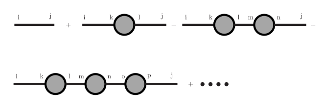
We now look at all contributions to the full propagators. First we recapitulate the charged propagator, , case. There we have that
| (14) |
because of the conservation of flavor. The lowest order propagator and the self-energy have the same flavor structure as Eq. (14). The sum over all diagrams for the charged propagators as depicted in Fig. 1 becomes a diagonal sum with no internal indices to be summed over. This resummation of the diagrams in terms of lowest order propagators and self-energy contributions becomes a simple geometric series. When summed, it gives a shift to the position of the pole of the lowest order propagator, see e.g. BDL . The position of this resummed pole defines the physical masses.
For the neutral sector the procedure is similar, but less straightforward due to the mixing. Neither the self-energy nor the lowest order propagator is diagonal, we thus need to keep the nine by nine structure as defined in Eq. (III.1). Consequently, the resummation has the structure
| (15) | |||||
as depicted in Fig. 1. If had been invertible it would have been a simple geometric series which could be resummed via matrix inversion as done e.g. in ABT2 . We perform below this resummation explicitly taking into account the exact structure of the matrices and . The simplest case with all valence quark masses equal and all sea quark masses equal is treated here, and is referred to as the (1+1) case following the notation used in our earlier work. The generalization to the more general cases can be found in App. B.
III.2 Matrix Structure of and .
For the (1+1) mass-case we are interested in, the expression simplifies considerably. By taking the appropriate mass limits it becomes
| (17) |
where is the unit matrix, is given by
| (18) |
and the two matrices are given by
| (19) |
The symbols denote the different types of propagator terms which remain after the mass limit has been taken, and are explicitly
| (20) |
and give the structure inside the various sectors as the matrix shown in Eq. (5). and give the sector structure as in Eq. (6). The contributions with correspond to the connected diagrams and those with to the disconnected diagrams when thinking in terms of quark lines. Similar remarks apply to all the other matrices discussed below.
Thus, one has a rather clean matrix structure for , involving just the three parameters . Furthermore, since is a projection operator, , one avoids arbitrarily high powers of .
Next, we investigate the matrix structure of the self-energy terms . In order to do this, we again turn the attention to the propagators . For the case of one flavor of valence quarks and one flavor of sea quarks, Sharpe and Shoresh Sharpe1 ; Sharpe2 showed that several constraints on the structure of follow from the (super)symmetries inherent in the PQ theory, and that the argument can be generalized to the more general cases. In App. A we show this extension expicitly. From this derivation follows that the block structure of the neutral sector, before the degree of freedom has been integrated out from the theory, can be written as
| (21) |
with
| (22) |
The symbols denote unknown functions, whose form we are not interested in for this discussion. We only need the structure of their arrangement in Eq. (21). Defining,
| (23) | |||||
| (24) |
one then finds that the matrix
| (25) |
is an inverse to . When checking this explicitly, it is useful to note that . This matrix is a straightforward generalization of the inverse given for the 1+1 flavor case in Sharpe2 .
If we now decompose as
| (26) |
where is the inverse of the lowest order propagator matrix, then corresponds to the sum of the one-particle irreducible self-energy diagrams. Since has the same block structure as , the inverse will have the same block structure as as well. Thus, subtracting from , one finds that has the same block structure as well, namely
| (27) |
where are different matrices from those in , but with the same matrix structure. The same structure should prevail after removing the degree of freedom Sharpe1 ; Sharpe2 . One can write in a convenient direct product-notation as well. From the definitions of one can rewrite them as
| (28) | |||||
| (29) |
where are as of yet unknown functions. With this notation, can finally be written as
| (30) |
where
| (31) |
Similar arguments show that is also the self-energy needed for the off-diagonal or charged meson with both quarks having the same mass.
III.3 The resummation
We now perform the resummation of Eq. (15). Since is a projection operator, a typical term in the sum looks like
| (32) |
Both and are diagonal, the first part thus resums component by component as a geometric series, giving
| (33) |
The “-part” seems less trivial. Writing out a few of the terms in a symbolic manipulations program such as Maple, one quickly sees a recurring structure which suggest a simple formula for the general term. Having this formula, a proof that it holds for all orders then follows by induction. Denoting each block of by we now list the resulting expressions for each sector and resum them. First, the sectors and , i.e. , all result in the same expression for a typical term giving
| (34) |
where . For convenience, now divide into three parts
| (35) |
with
| (36) |
For , note that
| (37) |
Using this and the definition of from Eq. (20), it follows that the resum into
| (38) |
Similarly, the combine to
| (39) |
and, since has a double pole, the sum up to
| (40) |
In all, we thus have the result
| (41) | |||||
The other sectors are not needed for this paper, since they do not contain any double pole contributions. However, we still list the full result here for completeness. Proceeding in the same way, we get that the neutral sector resummed propagator becomes
| (42) |
where the two matrices are given by
| (43) |
The symbols denote the various resummed propagator terms, given by
| (44) |
We see that the full propagator has exactly the same structure as the lowest order propagator in this simplest mass case. The resummed propagator matrix involves the three parameters , which are the direct counterparts to the lowest order parameters of .
III.4 from
We now expand the double pole around the position of the pole. The position is the same as the charged mass squared since is also the self-energy for that case. The position of the zero of we thus refer to as . It is the physical mass of the charged mesons (in the degenerate mass-case, there is only one such mass). We expand around the double pole term and get
| (45) |
The renormalization factor is defined as
| (46) |
Here and below we have indicated the dependence on the momentum and the of the various quantities. They also depend on the LECs of PQPT. The definition of in (45) coincides with the one given in Eq. (2).
IV Analytical results for
Equation (47) is written in terms of the blocks of , but for the explicit calculations we want to have the expression in terms of the self-energies directly, since this is what we know how to calculate. In the degenerate case we are studying in this paper, there are several equivalent ways to obtain the quantities needed since and appear in many different elements of the full self-energy matrix. We chose to use
| (48) |
which follows immediately from Eqs. (30) and (31). Then we get
| (49) |
IV.1 at NNLO
For the NNLO calculation of , we have to determine the expression for (49) up to . This means that all quantities appearing in Eq. (47) have to be expanded up to the appropriate order.
The first terms are of the form . Here is of , so we have to determine up to . From the definition of and , we get
| (50) |
The expressions for can be written as a string of terms which denote the 1PI diagrams of progressively higher order.
| (51) |
where contains derivatives of the self-energy diagrams of , and derivatives of those of . Note that differentiation lowers the order of the diagram contributions by two, and therefore these terms are of and respectively. It is sufficient to use the lowest order mass instead of in since the differentiated diagrams in that term are already of . However, in the case of the argument should be expanded in a Taylor series around , since the diagrams in are of . If is formally written as
| (52) |
then an expansion of up to gives
| (53) | |||||
where represents the NLO correction to the lowest order charged meson mass, which is given by . In practice, however, this Taylor expanded term is not needed, because contains no higher powers of , and thus the derivative term of (53) is identically zero.
Collecting the relevant terms up to gives
| (54) |
Next, the form of has to be determined up to . In order to do this, we determine up to , multiply the expressions for and together and collect the resulting terms up to . As for the terms we write the self-energies as a string of terms of progressively higher order:
| (55) |
For the argument must be expanded in a Taylor series around , since the diagrams in are of . An expansion of up to gives
| (56) | |||||
where again represents the NLO correction to the lowest order charged meson mass, given by .
Thus, up to , the ’s are given by
| (57) | |||||
where the last two terms are of and represent the NNLO contributions. For convenience, we will use the notation for the derivative term, assuming it understood that the derivative is as in Eq. (57).
Having this result, we now get the final expression for up to to be
| (58) | |||||
Putting everything together, the analytical expression for up to , or NNLO, is given by
| (59) | |||||
where the arguments of the functions have been suppressed.
IV.2 Expression for
The analytical expression for is given to NNLO in the form
| (60) |
where the and contributions have been separated. The NNLO contribution has been further split into the contributions from the chiral loops and from the counterterms or LECs.
It should be noted that we have chosen to give the results to the various orders in terms of the three flavor lowest order decay constant and in terms of the lowest order meson masses, since these are the fundamental inputs in PQPT. The situation is different in standard PT, where the main objective is comparison with experiment, in which case the formulas are most often rewritten in terms of the physical decay constants and masses. We have changed here the general to as is appropriate for the three flavor case.
The lowest order contribution to is just the difference between the valence sector quark mass and the sea sector quark mass, i.e
| (61) |
Here one sees explicitly the fact that this is a quantity relevant only in the partially quenched theory, since the lowest order contribution vanishes when one takes the limit of unquenched PT. We have checked that this also holds for the and contributions.
V Numerical Results and Discussion
V.1 Checks on the Calculation
As for the previous articles on NNLO calculations in PQPT, the calculations are rather lengthy, and require careful checking procedures to avoid the possibility for mistakes showing up in the end result. The complete calculations have therefore been performed in two complete independent versions, which have been checked against each other for agreement. The numerical results have been treated likewise, and the programs were written in different programming languages (Fortran and C++). Furthermore, the divergence structure agrees with general calculation of BCE2 and the cancellation of nonlocal divergences happens as required. The end results are expected to vanish for , since the quantity is a quantity relevant for the PQ theories only. This has been shown both for the and analytical formulae and checked numerically as well. The latter can also be seen from the fact that the contour plots below do not show a peaked behavior near the diagonal where .
V.2 The Numerics
All plots in this section are given in terms of the relative shifts to the lowest order contribution . That is, we plot
| (65) |
where we keep the contributions in Eq. (60) up to and including when we refer to the NLO case and up to and including when we refer to the NNLO case.
In the long run, the input parameters should be determined by fits of the PQPT formulas to lattice QCD data. These fits are not available at present, although suitable simulation results should become available in the near future. So we present here plots with the same choices of input parameters as in BDL ; BL1 ; BL2 ; BDL2 . This is mainly from the NNLO fit to experimental data, referred to as “Fit 10”, which is presented in Ref. ABT2 . That fit has MeV and a renormalization scale of MeV. The NNLO LECs and the NLO LECs and were not determined in that fit and they have been set to zero for simplicity. It should be noted that cannot be determined from experimental data, since it is a distinguishable quantity only in the PQ theory. Some recent results on and have been obtained in Ref. piK , but they have nevertheless been set to zero in the plots in this paper, since the present numerics are mainly intended for illustrative purposes.
For the degenerate mass-case we are working with in this article, we have only two input parameters for the quark masses, namely and . This allows for exhaustive contour plots of the whole parameter region of interest. A contour plot of the NLO relative correction is given in Fig. 2, and in Fig. 3 the same parameter region is plotted for the sum of the NLO and the NNLO shifts. Let us remind the reader here that the quantities correspond to lowest order meson masses squared. For the NNLO case, diagrams appear which can have on-shell intermediate states for . For that part of the plot we have simply kept the real part only of the relevant sunset integral. The error due to this should be a small effect, similar in size to the width compared to the mass of the eta for realistic quark masses.
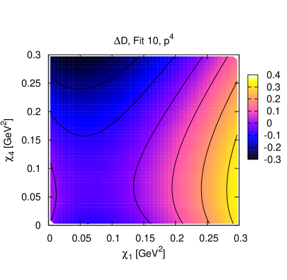
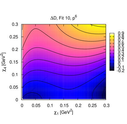
The plots show a reasonable convergence behavior for when both . Furthermore, as mentioned above, since we have plotted the relative correction with respect to the lowest order contribution , the plots would have a peaked limiting behavior near the diagonal line if the NLO or NNLO corrections were nonzero for . That this is not the case is clear from the plots, and in agreement with the expected result. Furthermore, the general shape of the contour over the plotted parameter space is rather different for the NLO and the NNLO results, in particular, the contributions are rather sizable. This is an expected result as well, since previous calculations of the masses and decay constants to NNLO show exactly this behavior. In Ref. BDL2 it was shown that the type of behavior is strongly dependent on the values of the largely unknown NNLO LECs and an example of changes in some of the less well determined LECs was given that improves the convergence behavior dramatically.
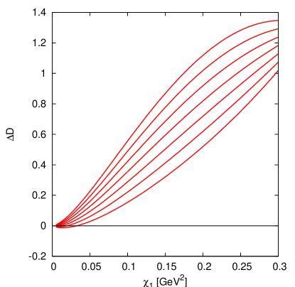
However, since a major point of this article is the dependence on the LEC for , we have, in addition to the contour plots, chosen a parameter line in the two-dimensional mass-space, where results for different values of the LECs have been plotted. This parameter line is defined by
| (66) |
This choice is motivated by the fact that the sea quark mass is usually taken to be larger than the valence quark mass in lattice simulations.
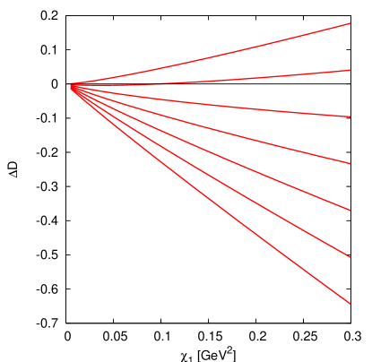
In Fig. 4 the NLO relative correction has been plotted along this parameter line, as a function of . The plot is for several different values of the LEC , ranging between zero and . All other parameters are set to the values of “Fit 10”. Convergence as , for all values of , is evident, in agreement with the contour plot. The dependence on is exactly linear as expected from Sharpe2 and Eq. (62).
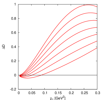
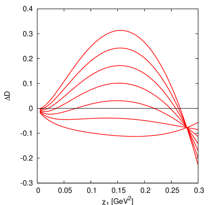
In Fig. 5, the NNLO relative correction is plotted using the same values for the LECs, namely “fit 10”, except for . As a comparison, Fig. 6 shows the NNLO relative correction with all LECs, except , set to zero. As anticipated from the contour plot, the contribution is sizable in both cases, but with a somewhat lower overall amplitude when the LECs are set to zero. Also for the NNLO results, we have an exact linear dependence on as can be seen from Eq. (IV.2). As already discussed, the large amplitude of the NNLO corrections is not expected to be a concern for the convergence of the theory, since many of the LECs are as of yet poorly determined. As an example to show this as well as the subtraction scale dependence, we have shown in Fig. 7 the NNLO relative correction as a function of and all other LECs set to zero at a subtraction scale GeV.
VI Fitting strategies
VI.1 LECs relevant for the eta mass
The eta mass to NNLO in PT was calculated in ABT2 and to NLO in GL2 . We present here the corrections in the form with the dependence written in terms of lowest order masses and decay constants as calculated in ABT2 and obtainable from website . The NLO part depending on the LECs is
| (67) | |||||
The occur in the three combinations , and .
The NNLO part depending on the NNLO LECs is
| (68) | |||||
VI.2 Obtaining LECs from : fitting strategies
In Ref. BDL2 we discussed at some length, possible fitting strategies for determining the various LECs at and . In the analytical expressions for some additional LECs are present, which motivates further elaboration on these fitting strategies. At the only new LEC is and at we now have and as well. It turns out that together with the expressions for it is possible to determine all the combinations of LECs which appear in the NLO+NNLO expressions for the masses including the eta mass. We will now give a short outline of how one might proceed but we will concentrate on the masses only.
From the charged masses we have the dependence
| (70) |
In these expressions, denotes the average over the sea-sector quarks, and the superscripts indicate having 2 nondegenerate valence quark masses and 3 nondegenerate sea quark masses. We refer to the discussion in Ref. BDL2 for details on which mass degeneracies which are needed for the determination of the LECs, and just refer to the needed expressions here.
The NLO result for is proportional to
| (71) |
from which an overall factor of has been removed. The resemblance to the mass expressions is striking, even though the coefficients are not quite the same. However, it is clear that all combinations needed to determine the eta mass at NLO can now be obtained. Since we can obtain from the decay constant we can also get at separately. This was already shown to NLO in Sharpe1 ; Sharpe2 .
Let us now do the same thing for the NNLO LECs. The situation is somewhat more involved but not different in principle. The full discussion can be found in BDL2 , we only present a part of it here. The mass at NNLO for the (2+2) case there depended on the NNLO LECs as
| (72) | |||||
The combinations are defined as
| (73) |
From Eq. (72) it is clear that the combinations to can be determined from the charged masses at NNLO by varying the input quark masses in the lattice QCD simulations. The above is a rephrasing of the discussion of BDL2 .
Let us now rewrite the NNLO LECs contribution to in the same fashion. Eq. (63) can be rewritten as
| (74) | |||||
It is clear that from we can thus determine the remaining LECs needed to get at the eta mass at NNLO. We can easily get at the missing combinations and .
VII Conclusions
In this paper, we have calculated the quantity to NNLO. This quantity was first proposed and calculated to NLO by Sharpe and Shoresh Sharpe1 ; Sharpe2 , as a way to obtain a better fit of the LEC , since it appears already at NLO for this quantity. This then also allowed to get the eta mass at NLO in PT. As discussed in Sharpe1 , is a well defined Lattice quantity in terms of the correlation function .
We have presented the full analytical results for to NNLO, together with a numerical analysis indicating the typical size of the corrections for various choices of the LECs. In particular, we demonstrate the sensitive dependence on the LEC which these expressions exhibit, both at NLO and at NNLO. It should also be noted that, in addition to showing dependence on the LEC already at NLO, the NNLO analytical expressions presented here also depend on the LECs and , none of which were present in the NNLO expressions for the charged masses or decay constants.
We have extended the discussion about possible fitting strategies in Ref.BDL2 to include the new LECs which appear in the NNLO results for . The conclusion is that the NLO and NNLO expressions for the charged masses and decay constants, together with the expressions for provided in this article, in fact give enough information to determine all of the combinations of LECs which appear in these calculations, including those for the eta mass at NNLO.
In addition we have also shown how to resum explicitly the full propagator from the lowest order propagator and self-energies also in the case for the neutral propagator in PQPT.
Acknowledgments
The program FORM 3.0 has been used extensively in these calculations FORM . This work is supported by the European Union TMR network, Contract No. HPRN - CT - 2002 - 00311 (EURIDICE) and the EU - Research Infrastructure Activity RII3 - CT - 2004 - 506078 (HadronPhysics).
Appendix A Symmetry Constraints on the propagator
In Ref. Sharpe2 , App. E, a number of constraints on the form of the meson propagators in PQQCD were derived. The Lagrangian of QCD played no role, since the only properties of the quark bilinears which were used were the transformation properties under vector symmetries, whose properties are shared by the meson fields of PQPT. It was then argued that the derivation presented in Sharpe2 could easily be extended to the case with more than one flavor of valence quarks and nondegenerate masses. We will now show this generalization to the general case with valence and ghost quarks and sea quarks. The masses are fully general except that the -th ghost quark has the same mass as the -th valence quark mass for all . Three types of symmetries are needed, all fairly trivial extensions of the ones in Sharpe2 .
We suppress the time ordering and often the space-time dependence in the remainder of this appendix to make the symmetry structures more visible.
A.1 Phase rotations and
We write the quark flavors as a vector
| (75) |
where indices to denote the valence quarks. Indices to denote the sea quarks and indices to denote the bosonic “ghost” quarks.
The direct generalization of the subgroup of the vector transformations in Ref. Sharpe2 , is
| (76) |
Under a phase rotation of only the flavor , transforms as
| (77) |
The invariance of implies that the indices must be paired up. Thus, non-vanishing elements of have the form or .
A second relation which can be simply derived is that is a symmetric matrix. Consider
| (78) | |||||
which make use of rotation invariance and translation invariance. The minus sign in the last step is only needed when both and are fermionic fields. This equation implies that . In particular, this implies that defined in (III.1) is a symmetric matrix.
At this level has the structure
| (79) |
are symmetric matrices. The matrices are ordered in the valence, sea and bosonic sectors.
A.2 transformations
The third type of symmetries is transformations involving the -th quark from the valence sector and the -th quark from the bosonic sector . There are of such symmetries. Below we will use the label and to denote these quarks respectively.
This type of transformations is of the form
| (80) |
where are commuting numbers, are anticommuting numbers and satisfies . Here we think of it as acting on the vector
| (81) |
The index in (80) indicates which we are referring to.
This type of symmetry transformations can, together with the previous symmetries, be used to set further constraints on the block structure of . In order to see this, we first form the following classes of 2-indexed objects out of elements of :
| (82) |
where indicates the -th index in the sea sector, and the matrix indices take both take values from so as to form a supermatrix (or graded) structure. The symbol gives the correct sign of the graded symmetry, i.e. for and for the remaining ones. The objects in( 82) are the direct generalizations of the objects in Sharpe2 to the general flavor case.
In addition to these, we will also need the two classes of objects defined by
| (83) |
Here, the value chosen for must be different from the value chosen for and different from . The subscripts and indicate that is a valence index and a ghost index. All the objects defined above transform under as
| (84) |
Since is a symmetry, the expressions are invariant under these transformations. Writing out these transformations explicitly one arrives, after some calculations, at a number of constraint equations, which must be satisfied, for the symmetry to hold. Solving these equations, the constraints following from (82) are
| (85) | |||||
where as defined above, is the -th valence quark index is the -th ghost quark index and is the -th sea quark index. What we have shown so far is that the matrices and in (79) are identical and that the diagonal parts of and are the same.
The previous was a simple extension of what was done in Sharpe2 . The really new part is that for the general flavor case, we also have a distinction between diagonal elements and non-diagonal elements in the various matrices of . The invariant objects in (83) provides information about the matrix structure of these. Writing out the transformation (84) for these objects yields the additional constraint equations
| (86) |
for . These equations imply that the off-diagonal part of vanishes and that the off-diagonal parts of and are the same.
To summarize, has the structure
| (87) |
are symmetric matrices and is diagonal.
Here we can see that since and connect different sectors they are disconnected if we think in terms of external quark lines. That is from connected lines and related to charged propagators is a little more involved to show. First, we use the fourth line in Eq. (85) where we have an obviously charged object in the propagator. We now set a second valence/ghost quark to the same mass, i.e. . We can then use the permutation symmetry to turn the indices into . The final step is to use the symmetry to rotate the index back to .
| (88) |
which is the desired relation between and the charged meson propagator.
A.3 Equal mass limits
When masses are equal, we have more symmetries.
For all valence quark masses equal we can interchange two indices and everywhere and should remain invariant. This implies that we can interchange columns in and of Eq. (79). It also implies that must be invariant under the simultaneous change of a pair of columns and rows.
For all bosonic quark masses equal we can interchange two indices and everywhere and should remain invariant. This implies that we can interchange rows in and of Eq. (79). It also implies that must be invariant under the simultaneous change of a pair of columns and rows.
For all sea quark masses equal we can interchange two indices and . This means that and are invariant under the interchange of rows and that is invariant under the simultaneous interchange of rows and columns.
Putting the above together with and derived earlier shows that and are matrices with all elements equal. was diagonal so all its diagonal elements must be equal. For it implies that all diagonal elements are equal and that all off-diagonal elements are equal. The matrix then has precisely the structure of Eq. (22).
Appendix B The resummation in the general case
In this appendix we show how to do the resummation in the general case for an arbitrary number of valence quarks and sea quarks .
The general lowest order neutral propagator matrix (16) can be written in the form
| (89) |
The notation here is similar but not the same as in the main text. The matrices and are diagonal matrices with propagators.
| (90) |
The the various symbols are the valence and ghost sectors and the sea quark sector. In the equal mass limit Eq. (89) reduces to Eq. (17).
The self-energy has the structure derived in App. A where the submatrices now have a more general structure than in the main text.
| (91) |
is a symmetric by matrix. is a symmetric by matrix. is a diagonal by matrix. is a by matrix. and have only disconnected, only connected parts when thinking in terms of the external quark lines. has contributions from both.
The full propagator in the neutral sector is the sum
| (92) |
Not all parts in will appear in the final resummation to all powers. We thus need to extract the parts that appear to all orders similar to what was done in the main text by splitting into and . We do it here by splitting into four parts with different properties.
| (93) |
with
| (97) | |||||
| (101) | |||||
| (105) | |||||
| (110) |
We define four general types of structures
| (115) | |||||
| (119) | |||||
| (123) | |||||
| (128) |
The matrices and column vectors stand here for a generic form. These various types satisfy matrix multiplication properties.
-
•
A product of a type I matrix with another one of type I,II,III,IV is of type I,II,III,IV respectively. This is true for multiplication by type I from front or back.
-
•
A product of a type II matrix with another one of type II,III,IV is zero. This is true for multiplication by type II from front or back.
-
•
A product of two type III matrices is of type II.
-
•
A product of type IV with type I,III,IV is of type IV.
The first property allows to treat the part similarly to the in the main text. We resum it separately and define
| (129) |
Due to the diagonal structure of and this resummation can be done with
| (130) |
The second property means that can only appear once, and together with the third means that multiplied by itself or products of appears at most twice. Putting then all strings of only together in the sum can be rewritten as
The remaining summation in (B) can be done by noticing that
| (132) |
The quantity in the last bracket is a scalar and can be taken out of the matrix products in the partial sum. The sum then can be done by a geometric series in only the quantity in the last set of brackets.
The remaining part of the calculation is to perform all of the matrix multiplications. Some properties that are used heavily to bring the result into its final form are
| (133) |
There are similar properties for the and combinations.
The result can be written in a form reminiscent of the lowest order (89).
| (134) |
where the matrices have the same structure as the matrices in (91). These are given in terms of the self-energy and lowest order propagator parts as
| (135) |
Eqs. (134) and (B) are the main results of this appendix. Note that all lowest order poles have been shifted to the resummed poles everywhere where they appear. We have also checked that the results of this appendix agree with those in the main text by taking the various equal mass limits.
References
- (1) S. Weinberg, Physica A 96, 327 (1979);
- (2) J. Gasser and H. Leutwyler, Ann. Phys. 158, 142 (1984);
- (3) J. Gasser and H. Leutwyler, Nucl. Phys. B 250, 465 (1985).
- (4) A. Morel, J. Phys. (France) 48, 1111 (1987).
- (5) C. W. Bernard and M. F. L. Golterman, Phys. Rev. D 46, 853 (1992) [arXiv:hep-lat/9204007].
- (6) S. R. Sharpe, Phys. Rev. D 46, 3146 (1992) [arXiv:hep-lat/9205020].
- (7) C. W. Bernard and M. F. L. Golterman, Phys. Rev. D 49, 486 (1994) [arXiv:hep-lat/9306005].
- (8) S. R. Sharpe and N. Shoresh, Phys. Rev. D 62, 094503 (2000) [arXiv:hep-lat/0006017].
- (9) S. R. Sharpe and N. Shoresh, Phys. Rev. D 64, 114510 (2001) [arXiv:hep-lat/0108003].
- (10) J. Bijnens, N. Danielsson and T. A. Lähde, Phys. Rev. D 70, 111503 (2004) [arXiv:hep-lat/0406017].
- (11) J. Bijnens and T. A. Lähde, Phys. Rev. D 71, 094502 (2005) [arXiv:hep-lat/0501014].
- (12) J. Bijnens and T. A. Lähde, Phys. Rev. D 72, 074502 (2005) [arXiv:hep-lat/0506004].
- (13) J. Bijnens, N. Danielsson and T. A. Lähde, Phys. Rev. D 73, 074509 (2006) [arXiv:hep-lat/0602003].
- (14) S. Scherer, in Advances in nuclear physics, edited by J.W. Negele and E. Vogt (Kluwer Academic/Plenum Publishers, New York 2003), vol. 27, pp. 277-538 [hep-ph/0210398]; G. Ecker, hep-ph/0011026; A. Pich, hep-ph/9806303.
- (15) J. Bijnens, arXiv:hep-ph/0604043.
- (16) J. Bijnens, G. Colangelo and G. Ecker, Ann. Phys. 280, 100 (2000) [arXiv:hep-ph/9907333].
- (17) J. Bijnens, G. Colangelo and G. Ecker, JHEP 9902, 020 (1999) [arXiv:hep-ph/9902437].
- (18) G. Amorós, J. Bijnens and P. Talavera, Nucl. Phys. B 568, 319 (2000) [arXiv:hep-ph/9907264].
- (19) G. Amorós, J. Bijnens and P. Talavera, Nucl. Phys. B 602, 87 (2001) [arXiv:hep-ph/0101127].
- (20) J. A. Vermaseren, arXiv:math-ph/0010025.
-
(21)
The analytical formulas may be downloaded via:
http://www.thep.lu.se/bijnens/chpt.html.
The programs are available on request from the authors. - (22) J. Bijnens, P. Dhonte and P. Talavera, JHEP 0401, 050 (2004) [arXiv:hep-ph/0401039], JHEP 0405, 036 (2004) [arXiv:hep-ph/0404150].