Gluon flux-tube distribution and linear confinement in baryons

Abstract

The distribution of gluon fields in a baryon is of fundamental interest in QCD. We have observed the formation of gluon flux-tubes within baryons using lattice QCD techniques. In particular we use a high-statistics approach, based on the translational and rotational symmetries of the four-dimensional lattice, which enables us to observe correlations between the vacuum action density and the quark positions in a completely gauge independent manner. This contrasts with earlier studies which needed to use gauge-dependent smoothing techniques. We use 200 ${\cal O}(a^{2})$-improved quenched QCD gauge-field configurations on a $16^{3}\times 32$ lattice with a lattice spacing of 0.123 fm. Vacuum field fluctuations are observed to be suppressed in the presence of static quarks such that flux tubes represent the suppression of gluon-field fluctuations. We considered numerous different link paths in the creation of the static quark sources in order to investigate the dependence of the flux tubes on the source shape. We have analyzed 11 L shapes and 8 T and Y shapes of varying sizes in order to explore a variety of flux-tube topologies, including the ground state. At large separations, Y-shape flux-tube formation is observed. T-shaped paths are observed to relax towards a Y-shaped topology, whereas L-shaped paths give rise to a large potential energy. We do not find any evidence for the formation of a $\Delta$-shaped flux-tube (empty triangle) distribution. However, at small quark separations, we do observe an expulsion of gluon-field fluctuations in the shape of a filled triangle with maximal expulsion at the centre of the triangle. Having identified the precise geometry of the flux distribution, we are able to perform a quantitative comparison between the length of the flux-tube and the associated static quark potential. For every source configuration considered we find a universal string tension, and conclude that, for large quark separations, the ground state potential is that which minimizes the length of the flux-tube. The characteristic flux tube radius of the baryonic ground state potential is found to be $0.38\pm 0.03$ fm, with vacuum fluctuations suppressed by $7.2\pm 0.6\%$. The node connecting the flux tubes is 25% larger at $0.47\pm 0.02$ fm with a larger suppression of the vacuum by $8.1\pm 0.7\%$

I INTRODUCTION

Recently there has been renewed interest in studying the distribution of quark and gluon fields in the three-quark static-baryon system. While the earliest studies were inconclusive Flower:1986ru , improved computing resources and analysis techniques now make it possible to study this system in a quantitative manner Takahashi:2002bw ; Alexandrou:2001ip ; Alexandrou:2002sn ; deForcrand:2005vv . In particular, it is possible to directly compute the gluon field distribution Ichie:2002mi ; Okiharu:2003vt ; Bissey:2005sk using lattice QCD techniques similar to those pioneered in mesonic static-quark systems Sommer:1987uz ; Bali:1994de ; Haymaker:1994fm .

Similar to Okiharu and Woloshyn Okiharu:2003vt , our first interest is to test the static-quark source-shape dependence of the observed flux distribution, as represented by correlations between the quark positions and the action or topological charge density of the gauge fields. To this end, we choose three different ways of connecting the gauge link paths required to create gauge-invariant Wilson loops as in our preliminary study Bissey:2005sk . In the first case, quarks are connected along a T-shape path, while in the second case an L-shape is considered. Finally symmetric link paths approximating a Y-shape such that the quark positions approximate the vertices of an equilateral triangle are considered. The latter is particularly interesting as the probability of observing a $\Delta$-shape flux-tube (empty triangle) distribution is maximised in this equidistant case. The most recent lattice QCD studies are in favor of the Y ansatz when it comes to the confinement potential Takahashi:2002bw at long distances Alexandrou:2001ip ; Alexandrou:2002sn ; deForcrand:2005vv and flux tube formation Ichie:2002mi . We also note that a theoretical calculation using center-vortex QCD with gauge group $SU(3)$ also favors the Y ansatz Cornwall:2006 . In order to better compare T and Y shapes we study configurations in which the quarks are in the same location and only the connection point changes. Such a direct comparison is not possible with the L-shape.

Because the signal decreases in an exponential fashion with the size of the loop, it is essential to use a method to enhance overlap with the ground state of interest. We use strict three-dimensional APE smearing APE87 to enhance the overlap of our spatial-link paths with the ground-state static-quark baryon potential. Time-oriented links remain untouched to preserve the correct static quark potential at all separations. We present results for two levels of source smearing including a minimal smearing of 10 APE steps and an optimal smearing of 30 APE steps. The comparison of two levels of smearing reveals interesting insight into the manner in which the flux tubes evolve to become the ground state.

Complete details of the construction of Wilson loops for the determination of the static quark potential and associated gluon-field distributions are presented in Sec. II. Sec. III presents the three-point correlation function calculated to reveal the response of the vacuum to the presence of quarks. Of particular importance is the insensitivity to the choice of metric such that the observation of vacuum field suppression is unambiguous.

Excellent signal to noise is achieved via a high-statistics approach based on translational symmetry of the four-dimensional lattice volume and rotational symmetries of the lattice as described in detail in Sec. IV. This approach contrasts with previous investigations, which used gauge fixing followed by projection to smooth the links and resolve a signal in the flux distribution Ichie:2002mi ; Okiharu:2003vt .

Sec. V presents the simulation results for sources constructed from 10-sweep smeared links. We find substantial correlation between the source and the observed field distribution. While these sources provide information vital to linking the flux-tube distribution to the static quark potential, they are not adequate to isolate the ground-state potential at large quark separations. Therefore in Sec. VI we complement these results with sources constructed from optimal 30-sweep smeared links. Here clear deformation of the T-shape source to a Y-shape configuration is illustrated. A quantitative analysis comparing the static quark potentials is used to identify the ground state and in Sec. VII the position, radius and expulsion extent of the flux tubes and the node connecting them are determined. A summary of our findings is provided in Sec. VIII.

II WILSON LOOPS

To study the flux distribution in baryons on the lattice, one begins with the standard approach of connecting static quark propagators by spatial-link paths in a gauge invariant manner. APE-smeared spatial-link paths propagate the quarks from a common origin to their spatial positions as illustrated in Fig. 1. The static quark propagators are constructed from time directed link products at fixed spatial coordinate, $\prod_{i}U_{t}(\vec{x},t_{i})$, using the untouched “thin” links of the gauge configuration.

The smearing procedure replaces a spatial link, $U_{\mu}(x)$, with a sum of $1-\alpha$ times the original link plus $\alpha/4$ times its four spatially oriented staples, followed by projection back to $SU(3)$. We select the special-unitary matrix $U_{\mu}^{\rm FL}$ which maximises ${\cal R}e\,{\rm{tr}}(U_{\mu}^{\rm FL}\,U_{\mu}^{\prime\dagger})$, where $U_{\mu}^{\prime}$ is the smeared link, by iterating over the three diagonal $SU(2)$ subgroups of $SU(3)$ repeatedly. In practice, eight iterations over the three subgroups optimizes the projected link to about 1 part in $10^{8}$.

We initially repeated the combined procedure of smearing and projection $10$ times, with $\alpha=0.7$. However, it will become clear that $10$ times is not enough to isolate the ground state of the three-quark static-quark potential at large quark separations. We have found that repeating the smearing-projection procedure $30$ times is effective in isolating the ground-state. In this case the string-tension of the three-quark potential matches that of the quark-antiquark potential. We will present for comparison, results for both $10$ and $30$ steps of APE-source smearing.

Untouched links in the time direction propagate the spatially separated quarks through Euclidean time. In principle, the ground state is isolated after sufficient time evolution. Finally smeared-link spatial paths propagate the quarks back to the common spatial origin.

The three-quark Wilson loop is defined as:

$$W_{3Q}=\frac{1}{3!}\varepsilon^{abc}\varepsilon^{a^{\prime}b^{\prime}c^{\prime}}\,U_{1}^{aa^{\prime}}\,U_{2}^{bb^{\prime}}\,U_{3}^{cc^{\prime}},$$ (1)

where $U_{j}$ is a staple made of path-ordered link variables

$$U_{j}\equiv P\exp\left(ig\int_{\Gamma_{j}}dx_{\mu}\,A^{\mu}(x)\right)\,,$$ (2)

and $\Gamma_{j}$ is the path along a given staple as shown in Fig. 1.

Figure 1: Gauge-link paths or “staples,” $U_{1}$, $U_{2}$ and $U_{3}$, forming a three-quark Wilson loop with the quarks located at $\vec{r}_{1}$, $\vec{r}_{2}$ and $\vec{r}_{3}$. $\varepsilon^{abc}$ and $\varepsilon^{a^{\prime}b^{\prime}c^{\prime}}$ denote colour anti-symmetrisation at the source and sink respectively, while $\tau$ indicates evolution of the three-quark system in Euclidean time.

In this study, we consider several two-dimensional spatial-link paths. Figures 4 and 4 give the projection of T and L shape paths in the $x$-$y$ plane. Figure 4 shows the paths considered in constructing the Y-shape. In all cases the three quarks are created at the origin, $O$ (white bubble), then are propagated to the positions $Q_{1}$, $Q_{2}$ or $Q_{3}$ (black circle) before being propagated through time and finally back to a sink at the same spatial location as the source ($O$).

Figure 2: Projection of the T-shape path on the $x$-$y$ plane.

Figure 3: Projection of the L-shape path on the $x$-$y$ plane.

Figure 4: Projection of the Y-shape path on the $x$-$y$ plane.

For the Y-shape we create elementary diagonal “links” in the form of boxes as shown in Fig. 5. The $1\times 1$ and $1\times 2$ boxes are the average of the two path-ordered link variables going from one corner to the diagonally opposite one. Taking both of these paths better maintains the symmetry of the ground state potential and therefore provides improved overlap with the ground state. We also consider $2\times 3$ boxes which are the averages of the possible paths connecting two opposite corners using $1\times 1$ and $1\times 2$ boxes. We may create further link paths in the future for use in bigger loops if it becomes necessary. Hence a diagonal staple is, in fact, an average of several “squared path” staples connecting the same end points.

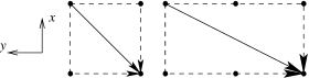
Figure 5: The diagonal path (solid line) is taken as the average of the two possible paths going around the box enclosing the end points.

The quark coordinates considered for Y and T shapes paths are summarised in Table 1. The Fermat point – the point within an acute triangle that minimizes the sum of the distances to the vertices – is also indicated. We note that the origin $(0,0)$ is not at the centre of these coordinates. Rather the coordinates are selected to place the quarks at approximately equal distances from each other. As one can see, the Fermat point, $F$, (also called the Steiner point in this particular case) is very close to the origin in most cases. In the table we also indicate the average inter-quark distance $\langle d_{qq}\rangle$ and the average distance to the Fermat point $\langle r_{s}\rangle$.

Note that in comparison to the measures considered in Ref. Alexandrou:2002sn , we have $L_{Y}=3\,\langle r_{s}\rangle$ and $L_{\Delta}=3\,\langle d_{qq}\rangle$. If the quark positions were on the vertices of an equilateral triangle, $L_{Y}$ and $L_{\Delta}$ would be linked in a simple linear fashion. In the quark configurations of Table 1, the quantity $\langle r_{s}\rangle$ is always within one part in a thousand of the radius of the circle circumscribing the triangle, therefore $\langle r_{s}\rangle$ is a good measure of the size of the baryon.

For the L-shape we have studied a small sample of 11 configurations, with $10$-step smearing. The following coordinates for the quarks are considered: $Q_{1}=(0,\ell)$, $Q_{2}=(0,0)$ and $Q_{3}=(\ell,0)$ where $\ell$ goes from $1$ to $11$. Because all L-shape triangles are simply a scaled version of a unique triangle, all distances in this shape are a given constant times the scale factor (here “$\ell$”) as in an equilateral triangle. In lattice units, we have $F=(\frac{3-\sqrt{3}}{6}\ell,\frac{3-\sqrt{3}}{6}\ell)$, $\langle r_{s}\rangle=\frac{1+\sqrt{3}}{3\sqrt{2}}\ell$, $\langle d_{qq}\rangle=\frac{2+\sqrt{2}}{3}\ell$ and the radius of the circumscribed circle is $\frac{\ell}{\sqrt{2}}$. The L-shapes are far further away from the ideal equilateral triangle than the T and Y shapes and $\langle r_{s}\rangle$ is not a good measure of the size of the baryon.

Table 1: $(x,y)$ coordinates for the three quarks considered for Y- and T-shape paths. We also show the coordinates of the Fermat point, $F$, and the average distance of the quarks from this point $\langle r_{s}\rangle$. Also shown is the average inter-quark distance $\langle d_{qq}\rangle$.

	$(x,y)$ Coordinates (lattice units)				Distance (fm)
#	$Q_{1}$	$Q_{2}$	$Q_{3}$	$F$	$\quad\langle r_{s}\rangle\quad$	$\langle d_{qq}\rangle$
1	$(1,0)$	$(-1,1)$	$(-1,-1)$	$(-0.42,0)$	0.15	0.27
2	$(2,0)$	$(-1,2)$	$(-1,-2)$	$(0.15,0)$	0.27	0.46
3	$(3,0)$	$(-1,2)$	$(-1,-2)$	$(0.15,0)$	0.31	0.53
4	$(3,0)$	$(-2,3)$	$(-2,-3)$	$(-0.27,0)$	0.42	0.72
5	$(4,0)$	$(-3,4)$	$(-3,-4)$	$(-0.69,0)$	0.57	0.99
6	$(5,0)$	$(-4,5)$	$(-4,-5)$	$(-1.11,0)$	0.72	1.25
7	$(7,0)$	$(-4,6)$	$(-4,-6)$	$(-0.54,0)$	0.88	1.52
8	$(8,0)$	$(-4,7)$	$(-4,-7)$	$(0.04,0)$	0.99	1.71

III GLUON FIELD CORRELATION

In this investigation we characterise the gluon-field fluctuations by the gauge-invariant action density $S(\vec{y},t)$ observed at spatial coordinate $\vec{y}$ and Euclidean time $t$ measured relative to the origin of the three-quark Wilson loop. We calculate the action density using the highly-improved ${\cal O}(a^{4})$ three-loop improved lattice field-strength tensor Bilson-Thompson:2002jk on four-sweep APE-smeared gauge links. While the use of this highly-improved action will suppress correlations immediately next to the quark positions, it will assist tremendously in revealing the flux-tube correlations which are the central focus of this investigation.

Defining the quark positions as $\vec{r}_{1}$, $\vec{r}_{2}$ and $\vec{r}_{3}$ relative to the origin of the three-quark Wilson loop, and denoting the Euclidean time extent of the loop by $\tau$, we evaluate the following correlation function

$$C(\vec{y};\vec{r}_{1},\vec{r}_{2},\vec{r}_{3};\tau)=$$ (3)

$$\quad\frac{\bigl{\langle}W_{3Q}(\vec{r}_{1},\vec{r}_{2},\vec{r}_{3};\tau)\,S(\vec{y},\tau/2)\bigr{\rangle}}{\bigl{\langle}W_{3Q}(\vec{r}_{1},\vec{r}_{2},\vec{r}_{3};\tau)\bigr{\rangle}\,\bigl{\langle}S(\vec{y},\tau/2)\bigr{\rangle}}\,,$$

where $\langle\cdots\rangle$ denotes averaging over configurations and lattice symmetries as described below. This formula correlates the quark positions via the three-quark Wilson loop with the gauge-field action in a gauge invariant manner. For fixed quark positions and Euclidean time, $C$ is a scalar field in three dimensions. For values of $\vec{y}$ well away from the quark positions $\vec{r}_{i}$, there are no correlations and $C\to 1$.

This measure has the advantage of being positive definite, eliminating any sign ambiguity on whether vacuum field fluctuations are enhanced or suppressed in the presence of static quarks. We find that $C$ is generally less than 1, signaling the expulsion of vacuum fluctuations from the interior of heavy-quark hadrons.

IV STATISTICS

In this investigation we consider 200 quenched QCD gauge-field configurations created with the ${\cal O}(a^{2})$-mean-field improved Luscher-Weisz plaquette plus rectangle gauge action Luscher:1984xn on $16^{3}\times 32$ lattices at $\beta=4.60$. The long dimension is taken as being the $x$ direction making the spatial volume $16^{2}\times 32$. Using a physical string tension of $\sigma=(0.440\ \text{GeV})^{2}=0.981\ \text{GeV}/\text{fm}$, the $q\bar{q}$ potential sets the lattice spacing to $a=0.123(2)$fm. In our previous study Bissey:2005sk we used $12^{3}\times 24$ lattices with the same action and parameter $\beta$.

To improve the statistics of the simulation we use various symmetries of the lattice. First, we make use of translational invariance by computing the correlation on every node of the lattice, averaging the results over the four-volume.

To further improve the statistics, we use reflection symmetries. Through reflection on the plane $x=0$ we can double the number of T and Y-shaped Wilson loops. By using reflections on both the plane $x=0$ and $y=0$ we can quadruple the number of L-shaped loops.

We finally use $90^{\circ}$ rotational symmetry about the $x$-axis to double the number of Wilson loops. This means we are using both the $x$-$y$ and $x$-$z$ planes as the planes containing the quarks.

In summary, the Y and T shape Wilson loop results are the average of $16^{3}\times 32\times 2\times 2\times 200=104,857,600$ Wilson loop calculations.

V SIMULATION RESULTS WITH 10 SWEEPS SMEARING

V.1 Qualitative results

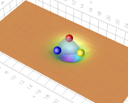
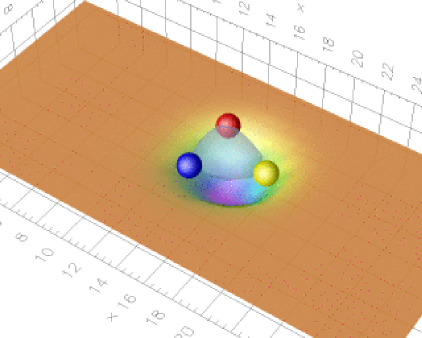
Figure 6: Expulsion of gluon-field fluctuations from the region of static quark sources illustrated by the spheres. An isosurface of $C(\vec{y})$ is illustrated by the translucent surface. A surface plot (or rubber sheet) describes the values of $C(\vec{y})$ for $\vec{y}$ in the quark plane, $(y_{1},y_{2},0)$. Results are for a 10-sweep smeared T-shape source with quark positions as in the third configuration of Table 1. The maximum expulsion is 9.7% and the isosurface is set to 4.9%.

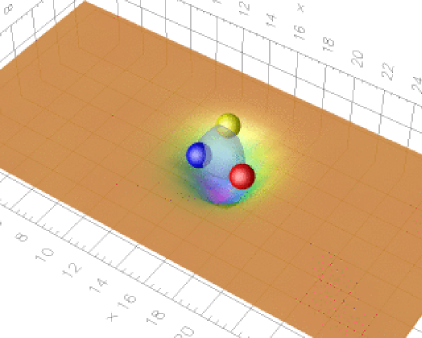
Figure 7: Isosurface and surface plot of $C(\vec{y})$ for a 10-sweep smeared Y-shape source with quark positions as in the third configuration of Table 1. The maximum expulsion is 9.8% and the isosurface is set to 4.9%. Further details are described in the caption of Fig. 8.

Figure 8: Isosurface and surface plot of $C(\vec{y})$ for a 10-sweep smeared L-shape source with quark separations of $\ell=3$. The maximum expulsion is 9.5% and the isosurface is set to 5.1%. Further details are described in the caption of Fig. 8.

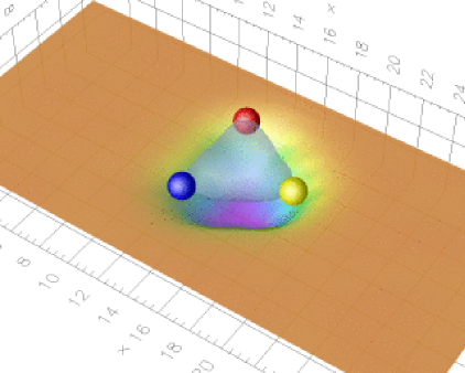
Figure 9: Isosurface and surface plot of $C(\vec{y})$ for a 10-sweep smeared Y-shape source with quark positions as in the fourth configuration of Table 1. The maximum expulsion is 8.9% and the isosurface is set to 4.5%. Further details are described in the caption of Fig. 8.

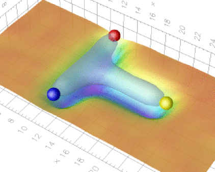
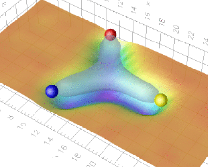
Figure 10: Isosurface and surface plot of $C(\vec{y})$ for a 10-sweep smeared T-shape source with quark positions as in the seventh configuration of Table 1. The maximum expulsion is 8.3% and the isosurface is set to 4.4%. Further details are described in the caption of Fig. 8.

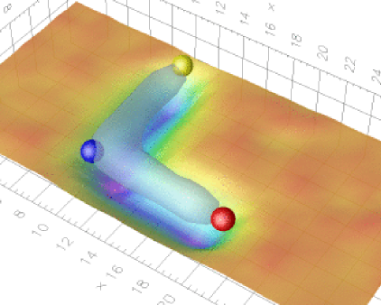
Figure 11: Isosurface and surface plot of $C(\vec{y})$ for a 10-sweep smeared Y-shape source with quark positions as in the seventh configuration of Table 1. The maximum expulsion is 8.3% and the isosurface is set to 4.4%. Further details are described in the caption of Fig. 8.

Figure 12: Isosurface and surface plot of $C(\vec{y})$ for a 10-sweep smeared L-shape source with quark separations of $\ell=10$. The maximum expulsion is 8.8% and the isosurface is set to 4.4%. Further details are described in the caption of Fig. 8.

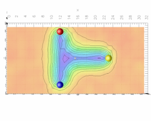
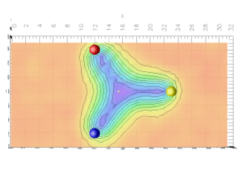
Figure 13: Contour plot of $C(\vec{y})$ for $\vec{y}$ in the quark plane, $(y_{1},y_{2},0)$, for a 10-sweep smeared T-shape source with quark positions as described in the seventh configuration of Table 1. The white diamond shows the position of the Fermat point.

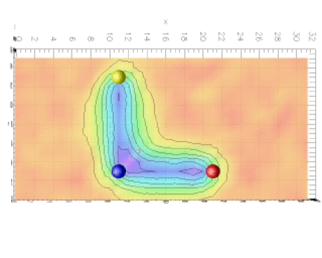
Figure 14: Contour plot of $C(\vec{y})$ for $\vec{y}$ in the quark plane, $(y_{1},y_{2},0)$, for a 10-sweep smeared Y-shape source with quark positions as described in the seventh configuration of Table 1. The white diamond shows the position of the Fermat point.

Figure 15: Contour plot of $C(\vec{y})$ for $\vec{y}$ in the quark plane, $(y_{1},y_{2},0)$, for a 10-sweep smeared L-shape source with quark separations of $\ell=10$. The white diamond shows the position of the Fermat point.

We begin by examining the correlation function $C(\vec{y};\vec{r}_{1},\vec{r}_{2},\vec{r}_{3};\tau)$ for 10-sweep smeared T-, Y- and L-shape sources at $\tau=2$. Larger time evolutions display the same features and are discussed further below.

At small quark separations, both the T- and Y-shape sources reveal a similar response of the vacuum to the quark positions. As seen in Figs. 8 and 8, isosurfaces of equal $C(\vec{y})$ form a bubble for quark positions in the third configuration of Table 1. Similar results are seen for smaller separations.

The isosurface for lower levels of field expulsion (i.e. further away from the quark positions) displays an approximately spherical shape as suggested by the surface plot for values of $\vec{y}$ just outside the quark positions.

In these figures we also show the value of $C(\vec{y})$ for $\vec{y}$ in the quark plane, $(y_{1},y_{2},0)$, on a surface plot (or rubber sheet). We clearly see that $C(\vec{y})$ is less than $1$ in the bubble, indicating an expulsion or suppression of vacuum gluon-field fluctuations.

These features are also seen to some extent for the L shape up until $\ell=3$ as shown in Fig. 8. These results correspond to a radius of about 0.3 fm or under.

At these small separations, one has the luxury of exploring the Euclidean time evolution of $C(\vec{y};\vec{r}_{1},\vec{r}_{2},\vec{r}_{3};\tau)$. While the depth of the vacuum field expulsion increases in going from $\tau=2$ to 4, it saturates in going from 4 to 6. In all cases however, there is no discernible change in the shape of the expulsion. Normalized contour plots of $C(\vec{y};\tau)$ are independent of $\tau$ to an excellent approximation.

With the fourth set of quark coordinates the bubble loses more of its symmetry and a filled triangular shape emerges as in Fig. 9, which corresponds to a radius of about 0.4 fm. This transition occurs at a radius of 0.35 fm for the L shape. However, this shape is much less symmetric to start with, as one of the inter-quark distances is 41% larger than the other two.

It is interesting to note the expulsion indicated by the suppression of $C(\vec{y})$ is largest at the centre of the quark configuration for all four quark-source shapes illustrated in Figs. 8 through 9. As such, there is no evidence of a $\Delta$-shape flux-tube (empty triangle) distribution forming at small distances. Rather, the vacuum expulsion observed in Fig. 9 is shaped as a solid or filled triangle as opposed to tubes. Here the inter-quark distance is more than 0.7 fm, which is outside the region where the potential is dominated by one-gluon exchange.

For radii larger than 0.5 fm we clearly see the formation of flux tubes as shown in Figs. 12 to 12. Here, a robust dependence of the observed flux-tube shape on the shape of the source is revealed. However, such a correlation is not surprising as these figures correspond to $\tau=2$. In principle, with sufficient time evolution these images will relax into the same ground-state configuration. In practice this is not possible as the signal is lost rapidly. Instead, one turns one’s attention to improving the source to best isolate the ground state, as we shall do in the following sections.

Nevertheless, some evolution of the flux tubes away from the source shape towards the Y-shape is already apparent. For example the flux-tube node of the T-shape source has moved by at least one lattice unit towards the Fermat point as illustrated in the contour plot of Fig. 15. Some curvature in the “top” of the T (left-most in the figure) is also apparent. In contrast, the observed Y shape of Fig. 15 is quite close to the source shape and the observed node of the flux tubes, which is very close to the origin, appears to have moved towards the Fermat point.

For the L shape results of Fig. 15 the issue is more subtle. While the node appears to have moved in the direction of the Fermat point to the next grid intersection, this observation might also be due to the suppression of the correlation near the quark positions associated with our use of a highly improved action.

While, Figs. 8 through 15 show the action-based correlation function results, we have also examined correlations of the Wilson loops with the topological charge, the squared colour magnetic field and squared colour electric fields, all of which are gauge invariant. The results are qualitatively similar and in some cases indistinguishable.

V.2 Quantitative results

We now move to a quantitative study of these results exploiting the knowledge of the node position from our qualitative analysis. We begin by determining the effective three-quark potential for the various quark positions, source shapes and Euclidean time evolutions. The vacuum expectation value for $W_{3Q}$ is

$$\langle W_{3Q}(\tau)\rangle=\sum_{n=0}^{\infty}C_{n}\exp(-a\,V_{n}\,\tau),$$ (4)

where $V_{n}$ is the potential energy of the $n$-th excited state and $C_{n}$ describes the overlap of the source with the $n$-th state. The effective potential is extracted from the Wilson loop via the standard ratio

$$a\,V(\vec{r},\tau)=\ln\left(\frac{W_{3Q}(\vec{r},\tau)}{W_{3Q}(\vec{r},\tau+1)}\right).$$ (5)

If the ground state is indeed dominant, plotting $V$ as a function of $\tau$ will show a plateau and any curvature can be associated with excited state contributions. Statistical uncertainties are estimated via the jackknife method Montvay:1994bk .

Our results for the various quark positions and source shapes are shown in Fig. 16. All small shapes are stable against noise over a long period of time evolution and even some of the largest shapes show some stability before being lost into the noise.

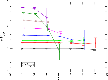
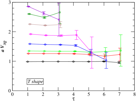
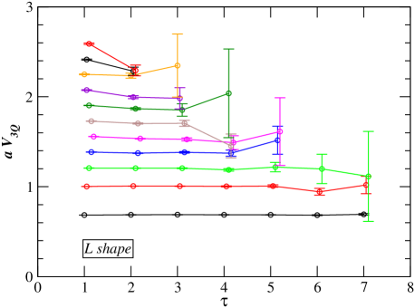
Figure 16: Effective static quark potential for 10-sweep smeared Y-, T- and L-shape sources. Some points are offset horizontally to increase readability. From bottom up, the lines correspond to shapes 1 through 8 of Table 1.

Robust plateaus are revealed for the first four quark positions of Table 1 for the T and Y shape sources. This suggests the ground state has been isolated and indeed the four lowest effective potentials of the T- and Y-shape sources agree. This result was foreseen in the qualitative analysis where Figs. 8 and 8 for the T- and Y-shape sources respectively displayed the same correlations between the action density and the quark positions.

Conversely, the disagreement between Figs. 12 and 12 indicates the ground state has not been isolated in one or possibly both cases. Indeed the nontrivial slopes of the seventh effective potentials of Fig. 16 for the Y- and T-shape sources confirm this. On the other hand, the curves are sufficiently flat to estimate an effective potential at small values of $\tau$, and given knowledge of the node position from our qualitative analysis, one can make contact with models for the effective potential.

The expected $\vec{r}$ dependence of the baryonic potential is Alexandrou:2002sn ; Takahashi:2002bw

$$V_{3Q}=\frac{3}{2}V_{0}-\frac{1}{2}\sum_{j<k}\frac{g^{2}C_{F}}{4\pi r_{jk}}+\sigma L\,,$$ (6)

where $C_{F}=4/3$, $\sigma$ is the string tension of the $q\bar{q}$ potential and $L$ is a length linking the quarks. There are two models which predominate the discussion of $L$; namely the $\Delta$ and Y ansätze.

In the $\Delta$-ansatz, the potential is expressed by a sum of two body potentials Alexandrou:2002sn . In this case $L=L_{\Delta}/2=3\langle d_{qq}\rangle/2$ where $L_{\Delta}$ is the sum of the inter-quark distances. In the Y-ansatz Takahashi:2002bw ; Ichie:2002mi , $L=L_{Y}=3\langle r_{s}\rangle$ is the sum of the distances of the quarks to the Fermat point.

In Figs. 19 and 19 we show the potentials from the different shapes at $\tau=1$ as functions of the inter-quark separation $\langle d_{qq}\rangle$ and the average distance to the Fermat point $\langle r_{s}\rangle$ respectively. In the case of the L-shape source, it is impossible to distinguish between the two ansatz from these figures as there is a linear relation between $\langle d_{qq}\rangle$ and $\langle r_{s}\rangle$. However, this is not the case for the T- and Y- shape sources. A linear or almost linear behavior for the long-distance potential is observed for Fig. 19 considering $\langle d_{qq}\rangle$ and similarly in Fig. 19 using $\langle r_{s}\rangle$. However, neither of these methods for expressing the inter-quark separation are capable of collapsing the potentials arising from T- Y- or L- shape sources to a single curve.

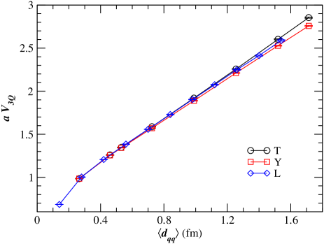
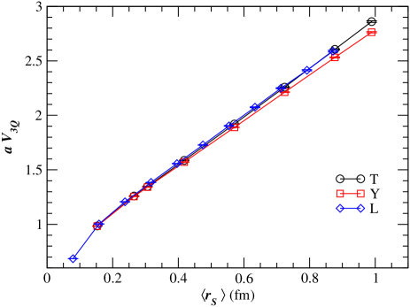
Figure 17: Effective potential at $\tau=1$ for various 10-sweep-smeared source shapes plotted as a function of the inter-quark separation $\langle d_{qq}\rangle=L_{\Delta}/3$.

Figure 18: Effective potential at $\tau=1$ for various 10-sweep-smeared source shapes plotted as a function of the average distance to the Fermat point $\langle r_{s}\rangle=L_{Y}/3$.

Figure 19: Effective potential at $\tau=1$ for various 10-sweep-smeared source shapes plotted as a function of the length of string connecting the quarks to the node location.

In Eq. 6, $L$ is meant to be the value of a length of string connecting the quarks (times a geometric constant for the $\Delta$ ansatz). Figs. 15 to 15 indicate that the actual node of the flux tube formation is not necessarily in the initial location shown in Figs. 4 to 4 nor, in the case of the T and L shapes, at the Fermat point. Using our knowledge of the node position in the observed state (which may not have relaxed to the ground state), we can determine the length of string required to connect the quark locations to the observed node position.

In the case of the Y-shape source, both the observed node and the source node are very close to the Fermat point. The difference in the total distance from the quark to the node is at most a few percent compared to $L_{Y}$. In the case of the T-shape source the observed node has moved by one lattice unit from the top of the T towards the Fermat point. In the smallest shape this means the node is extremely close to the Fermat point and that it is in the same location as the Y-shape node. In the case of the largest T-shape source considered in Table 1, the node may have moved more than one lattice unit.

In Fig. 19 we plot the potential of the various source shapes and sizes as a function of the total length of string connecting the quarks to the observed node. The length of string is computed as follows:

• For the T shape, it is computed as the total distance from the observed node moved one lattice unit from the top of the T towards the Fermat point.

• For the Y shape, it is taken to be equal to $L_{Y}$.

• For the L shape, it is taken to be $2\ell$ for the corresponding shape.

Using this measure on the $x$-axis, all the data points fall close to a single curve as displayed in Fig. 19. The three curves for T-, Y- and L-shape sources with the node movement included are extremely close to each other. The outstanding curve labeled “T (original node)” emphasizes the importance of including node movement identified by the three-point correlation function. This observation favours the Y-ansatz as providing the correct understanding of the nontrivial, nonperturbative dynamics of QCD.

The asymptotic part of all the curves follows a straight line as suggested by Eq. 6 and we can extract a string tension from this part. From the slope of the asymptotic part of these curves the string tension is $\sigma\approx 1.11\pm 0.01\ \text{GeV}/\text{fm}$. This is somewhat different from the results from Takahashi et al. Takahashi:2002bw of $0.89\ \text{GeV}/\text{fm}$ and also from the value we used to fix the lattice spacing ($0.981\ \text{GeV}/\text{fm}$). On the other hand, Ref. deForcrand:2005vv established that the Y-law describes the asymptotic potential with the same string tension as the $q$-$\overline{q}$ potential.

Since the Y shape source is already in a configuration providing access to the shortest string length, we must conclude that other aspects of the flux tube distribution have yet to evolve to become the ground state. Aspects including the flux-tube radius and the extent to which vacuum field fluctuations are suppressed inside the flux tube are examined in the following sections.

VI SIMULATION RESULTS WITH 30 SWEEPS SMEARING

Given that simple Euclidean time evolution to the ground state is difficult for large quark separations, we turn our attention to improving the source by adjusting the amount of spatial-link smearing used in the source construction.

For example, Takahashi et al. Takahashi:2002bw used a large amount of spatial smearing in their studies compared to our first study of 10 smearing-projection sweeps. We have found that an increase in the amount of smearing leads to a reduction in the value of the potential for large quark separations while the smaller separations ($r_{s}<0.5\ \text{fm}$) remain unchanged. This demonstrates that we have indeed isolated the ground state for the smaller shapes after 10 smearing sweeps, but not for the larger shapes.

Figure 20: Comparison of the potential of the Y shapes for 10 and 30 steps smearing. From bottom up, the lines correspond to shapes 1 through 8 of Table 1.

Figure 21: Comparison of the potential of the T shapes for 10 and 30 steps smearing. From bottom up, the lines correspond to shapes 1 through 8 of Table 1.

We therefore investigated systematically the effect of the smearing on the string tension. We find that the string tension decreases for increased smearing until it reaches a plateau at $30$ steps of smearing. The resulting value for $\sigma=0.97\pm 0.01\ \text{GeV}/\text{fm}$ is in agreement with the value used to fix the lattice spacing, $\sigma=0.98$ GeV/fm.

The increase in smearing provides excellent plateaus in the effective potential of the Y-shape source at the earliest times. This can be seen in Fig. 21 which provides a side-by-side comparison of 30 and 10 smearing sweeps for the effective potential obtained from the first three values of the time parameter $\tau$. Improved plateau behavior and lower effective potentials are observed for all separations.

Similar results are observed for the T-shape source as illustrated in Fig. 21. Figure 22 shows the complete time evolution of the potential of Y and T shapes for the 30 sweep smearing results. While it is clear that the ground state has not yet been reached for the largest T-shape source separations, it will be fascinating to observe how the T-shape source flux-tube distribution has evolved to produce a much lower effective potential.

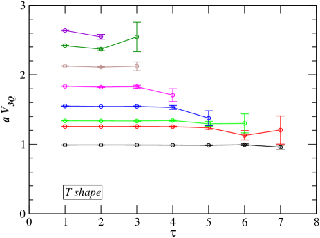
Figure 22: Study of the stability of the effective potential over Euclidean time for 30-sweep smeared Y and T shapes. From bottom up, the lines correspond to shapes 1 through 8 of Table 1.

The gluon-field distributions for the smaller source shapes are largely unchanged by the shift from 10 to 30 steps of smearing and we do not reproduce them here. However interesting results are revealed in the larger source shapes. The seventh configuration of Table 1 is depicted in Figs. 24 and 24 for the T- and Y-shape sources respectively.

The observed flux distribution of the T-shape source in Fig. 24 displays significant evolution towards the observed Y-shape of Fig. 24 (and not towards a $\Delta$ shape). The node connecting the quarks in the T-shape source has now moved two lattice units in the direction of the Fermat point rather than only a single unit as in the 10-sweep smearing case. While this is not so obvious in Fig. 24 it can be clearly observed in the contour plot of Fig. 26 and directly compared to Fig. 15. It is approaching the observed Y-shape source result of Fig. 26. In contrast, the Y-shape source flux-tube distribution is qualitatively unchanged, as can be seen in Figs. 24 and 26 compared to Figs. 12 and 15.

The isosurface of Fig. 24 and contour plot of Fig. 26 provide our best determination of the distribution of gluon flux tubes within the ground state of the static-quark baryon.

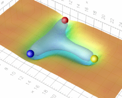
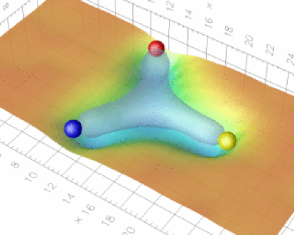
Figure 23: Expulsion of gluon-field fluctuations from the region of static quark sources illustrated by the spheres. An isosurface of $C(\vec{y})$ is illustrated by the translucent surface. A surface plot (or rubber sheet) describes the values of $C(\vec{y})$ for $\vec{y}$ in the quark plane, $(y_{1},y_{2},0)$. Results are for a 30-sweep smeared T-shape source with quark positions as in the seventh configuration of Table 1. The maximum expulsion is 6.4% and the isosurface is set to 4.4%.

Figure 24: Isosurface and surface plot of $C(\vec{y})$ for a 30-sweep smeared Y-shape source with quark positions as in the seventh configuration of Table 1. The maximum expulsion is 6.4% and the isosurface is set to 4.4%. Further details are described in the caption of Fig. 24.

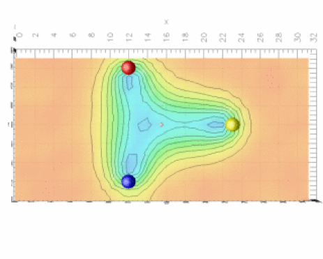
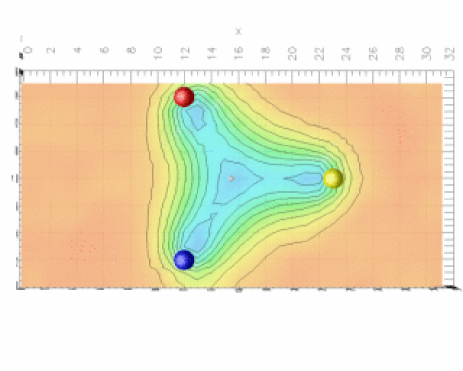
Figure 25: Contour plot of $C(\vec{y})$ for $\vec{y}$ in the quark plane, $(y_{1},y_{2},0)$, for a 30-sweep smeared T-shape source with quark positions as described in the seventh configuration of Table 1. The white diamond shows the position of the Fermat point.

Figure 26: Contour plot of $C(\vec{y})$ for $\vec{y}$ in the quark plane, $(y_{1},y_{2},0)$, for a 30-sweep smeared Y-shape source with quark positions as described in the seventh configuration of Table 1. The white diamond shows the position of the Fermat point.

Motivated by our earlier discovery and knowledge of the precise location of the flux-tube node, we plot the effective potential as a function of the total length of the piece of string connecting the quarks to the node in Fig. 27. The length of the piece of string is now computed as follows:

• For the Y shape, it is taken to be equal to $L_{Y}$.

• For the T shape, we first compute the total distance from a node moved one lattice unit from the base of the T.

• We also consider a curve for the T shape where the node is moved one lattice unit from the top of the T for small shapes (1 to 5 in Table 1) and two lattice units for the larger shapes.

These results which converge very well to a single curve are contrasted by a curve for the T shape where the length of string is computed from the source-node position located at the top of the T (original node).

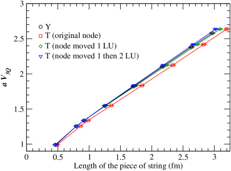
Figure 27: Effective potential at $\tau=1$ for various 30-sweep-smeared source shapes plotted as a function of the length of string connecting the quarks to the node location.

As can be seen in Fig. 27 the latter effective potential differs from the effective potential of the Y shapes. On the other hand, the two curves for the T-shape source with the node moved one or two lattice steps are very close together with the curve for the Y shapes. From this figure alone it is quite hard to decide which of the two moved T shapes is the closest to the Y shape. The following section providing a quantitative analysis of various cross sections of $C(\vec{y})$ will resolve this issue.

VII FLUX-TUBE PROPERTIES

Here the flux-tube and node properties as revealed by the three-point correlation function analysis in $C(\vec{y};r_{1},r_{2},r_{3};\tau)$ are quantitatively examined by considering several cross sections of $C$. In all cases $\vec{y}$ is constrained to the plane of the quarks $(y_{1},y_{2},0)$ and it is convenient to refer to these components as $(x,y,0)$ where $x$ is the coordinate of the long direction. For the remainder of this section the origin of the coordinate system is placed at the original position of the source node connecting the quarks in the computations.

We begin with a study of $C(x,y,0;\tau)$ with $\tau=2$ for a fixed value of $x$. Larger values of $\tau$ are examined below. In Fig. 28 we show the cross-section of the observed flux tube for the seventh T-shape source. Each curve corresponds to a fixed value of $x$. At $x=2$ we are at the edge of the observed node position. At $x=12$ we are past the quark in the long direction which is located at $x=11$. Results for both 10- and 30-sweep smeared T-shape sources are displayed.

Similarly, in Fig. 29 we show the cross-section of a flux tube observed for the seventh Y-shape source. Again, each curve corresponds to a fixed value of $x$. At $x=0$ we are close to the position of the node. At $x=9$ we are past the quark in the long direction which is located at $x=7$ in this case.

While the 10-sweep-smearing computations display stronger vacuum-field action suppression, the 30-sweep-smearing results display a larger flux-tube diameter. The latter also display a Gaussian shape in the vacuum-field suppression. We can also see enhanced action suppression near the location of the node and just before the position of the quark. While the latter feature is suppressed to some extent by our consideration of a highly-improved action density, the greater action suppression at the node is physically interesting. The convergence of the curves in the intermediate regime reflects the formation of a well defined flux tube.

For the T shape, the tube is reasonably well defined for $x=4$ through $7$ in both the 10- and 30-sweep-smeared sources. For the Y shape similar features appear for $x=2$ to $5$, again for both source smearings. We emphasize that it is the 30-sweep Y-shape source that provides the best overlap with the ground-state potential, as it is this source that provides the smallest and flattest effective potential. Therefore, the 30-sweep Y-shape source provides the best determination of the actual shape of the flux tube within the ground-state baryon system.

We can estimate the radius of the flux-tube by fitting a function of the form $1-A\,e^{-y^{2}/r^{2}}$ to selected curves in Figs. 28 and 29. For the T shape we choose to fit $x=5$ and similarly we select $x=3$ for the Y shape. All the non-linear fits hereafter have been done using the Levenberg-Marquardt method NRC92 . The results are summarised in Table 2. The fits are very good as illustrated by Fig. 30.

Table 2: Values of the fit parameters of the function $1-A\,\exp(-y^{2}/r^{2})$ to the curves $x=5$ of Fig. 28 and $x=3$ of Fig. 29. $r$ is reported in lattice units (LU) and fm. The last column indicates the area under $C(\vec{y})=1$ for the fitted curve in units of relative-depth times LU.

Shape	$A$	$r$ (LU)	$r$ (fm)	$Ar\sqrt{\pi}$
T (10 steps)	$0.070(1)$	$2.3(1)$	$0.28(1)$	$0.28(1)$
Y (10 steps)	$0.073(1)$	$2.2(1)$	$0.27(1)$	$0.28(1)$
T (30 steps)	$0.052(1)$	$3.3(1)$	$0.41(1)$	$0.31(1)$
Y (30 steps)	$0.055(1)$	$3.1(1)$	$0.38(1)$	$0.30(1)$

Our earlier observations about the depth and width of the flux-tubes for 10 versus 30 source-smearing sweeps are confirmed in Table 2. There is a significant correlation between the smeared-source size and the observed flux-tube radius. Whereas the source radius increases by 70% in going from 10 to 30 sweeps at a smearing fraction of 0.7, the observed flux-tube radius increases by only 40% for the Y-shape source. This indicates that some Euclidean time evolution of the flux-tube diameter has occurred in the 10-sweep smeared case, but not enough to relax to the true ground state captured by the 30-sweep smeared Y-shape source. Our best estimate of the ground-state flux-tube radius from the 30-sweep Y-shape source is $r=0.38(3)$ fm, where the uncertainty includes both statistical errors and the consideration of neighboring flux-tube cross-sections. Similarly, $A=0.055(2)$ for the relative vacuum expulsion in the flux tube of the seventh quark separation.

Finally in the last column we have the cross-sectional area created by the tube, computed from the fit. Despite rather different radii and depths observed for the two different smearing levels, this quantity is relatively uniform. The breadth of the 30-sweep-smeared sources does give rise to a larger expulsion of vacuum field fluctuations in the flux-tube of the action density distribution, despite the fact that these sources give rise to a lower static quark potential.

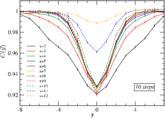
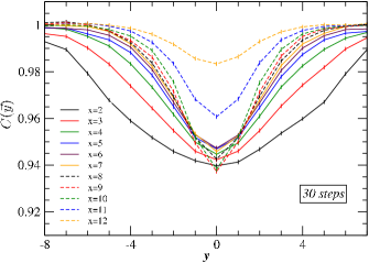
Figure 28: Value of $C(x,y,0)$ for the seventh T-shape source of Table 1 as a function of $y$ (the short direction of the quark plane) for various fixed values of $x$ (the long direction). Results from sources constructed from 10 (top) and 30 (bottom) sweeps of APE spatially-smeared links are compared. In these plots the origin is placed at the position of the node in the source.

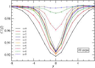
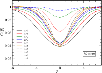
Figure 29: Value of $C(x,y,0)$ for the seventh Y-shape source of Table 1 as a function of $y$ (the short direction of the quark plane) for various fixed values of $x$ (the long direction). Results from sources constructed from 10 (top) and 30 (bottom) sweeps of APE spatially-smeared links are compared. In these plots the origin is placed at the position of the node in the source.

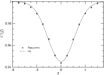
Figure 30: Example fit of a Gaussian to the flux-tube cross-section as per Table 2. The data points are for the seventh Y shape with 30 steps smearing as in the lower part of Fig. 29 but only for $x=3$.

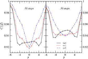
Figure 31: Value of $C(x,y,0)$ for the seventh T-shape source of Table 1 as a function of $y$ (the short direction of the quark plane) for various fixed values of $x$ (the long direction) near the top of the T-shape source. Results from sources constructed from 10 (left) and 30 (right) sweeps of APE spatially-smeared links are compared. The origin is placed at the position of the node in the source.

The observed flux distribution of the 30-sweep T-shape source in Fig. 24 displays significant evolution towards the observed Y-shape of Fig. 24 (and not towards a $\Delta$ shape). Further proof of this node displacement is presented in Fig. 31. Here the asymmetry about $x=0$ provides an estimate of the statistical errors. In both the 10- and 30-sweep cases on the $x=0$ line, we can see the response to the quarks on both sides of the top of the T at $x=\pm 6$ and less suppression of the vacuum action in the middle. This indicates the node has moved in both cases. However, in the case of 10 sweeps of smearing, the node is encountered already at $x=1$. On the other hand with 30 sweeps of smearing one observes a plateau which shows that the combined effect of the quarks and the node makes $C(\vec{y})$ constant. At $x=2$ where we pass through the position of the node, the dip from the node is clear but it is almost the same depth as the plateau at $x=1$.

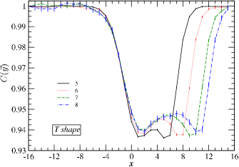
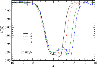
Figure 32: Value of $C(x,y,0)$ for a variety of T-shape (top) and Y-shape (bottom) sources of Table 1 as a function of $x$ (the long direction of the quark plane) for $y=0$ such that the centre of the node is encountered. Results are for the 30-sweep smeared sources. In these plots the origin is placed at the position of the node in the source.

Another perspective on the node properties is obtained by plotting the value of $C(x,y,0)$ along the line where the node and one quark stand on the long axis, $y=0$. We show this in Fig. 32 for several 30-sweep T- and Y-shape sources. In these plots the $x=0$ position indicates the original position of the node in the source.

In these figures we can typically observe two minima: one for the node on the left and one inside the quark position on the right. We choose to plot only the shapes for which these two features are resolved. For smaller shapes the node and quark peaks are not separable.

For the T shape the node moves first one lattice unit (shape 5) then two (shapes 6 to 8). On the other hand, for the Y-shape sources the node stays at its original location, indicating that the Y-shape source is already accessing the ground state.

A fit using the left-hand side of the nodes with an exponential curve of the form $1-A\,e^{-(x-x_{0})^{2}/r^{2}}$ can provide a more precise measure of the size of the node and of its actual location. The results have a slight dependency on the location of the cut in the data. In Table 3 we show the results of the fit for the seventh 30-sweep T- and Y-shape sources for two cuts. In cut I, only data from $-16$ up to the minima are kept. For cut II, data up to one lattice unit on the right of the minima are kept. Both fits are in good agreement with our data as is illustrated in Fig. 33.

Table 3: Values of the node fit parameters in the function $1-A\,\exp(-(x-x_{0})^{2}/r^{2})$ constrained to the left-hand side of the curves for the seventh 30-sweep T- and Y-shape sources in Fig. 32 for two data cuts. Cut I considers data from $x=-16$ to the minima and cut II from $-16$ to one lattice unit on the right of the minima. $r$ is reported in both lattice units (LU) and fm.

Shape	$A$	$x_{0}$ (LU)	$r$ (LU)	$r$ (fm)
T (Cut I)	$0.061(1)$	$+1.6(1)$	$3.7(1)$	$0.45(1)$
T (Cut II)	$0.062(1)$	$+1.8(1)$	$3.9(1)$	$0.48(1)$
Y (Cut I)	$0.062(1)$	$-0.5(1)$	$3.7(1)$	$0.45(1)$
Y (Cut II)	$0.063(1)$	$-0.2(1)$	$4.0(1)$	$0.49(1)$

Our best estimate of the ground-state node radius from the 30-sweep Y-shape source is $r=0.47(2)$ fm, where the uncertainty includes both the statistical error and the systematic uncertainty associated with the data cut. This value is 24(9)% larger than the flux-tube radius of $r=0.38(3)$ fm. In addition, we observe a 15(3)% increase in the amplitude of vacuum-action expulsion, $A$, in the node of the flux-tube relative to the expulsion observed in the flux tube itself, for the seventh quark separation. The amplitude of the relative action expulsion in the node is reasonably uniform for the various quark separations at $A=0.062(2)$. Here the uncertainty reflects statistical and systematic uncertainties associated with the data cuts and various quark separations.

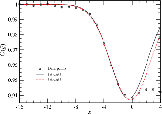
Figure 33: Example fit of a Gaussian to the flux-tube node as per Table 3. The data points are for the seventh Y shape with 30 sweeps of smearing as in the lower part of Fig. 32.

In these results $r$ is linked to the radius of the node which approaches 0.5 fm, a little larger than the flux-tube radius found earlier for the 30-sweep smeared sources. $x_{0}$ is indicative of the precise location of the node and Table 3 provides $x_{0}=1.7(1)$ LU for the T shape, consistent with the results of Fig. 27 and in accord with the contour plot of Fig. 26.

For the Y shape, Table 3 shows the node is very close to the origin defined at the node of the source. The movement of the observed node position to the left is consistent with movement towards the location of the Fermat point. In this case the Fermat point is located at $x=-0.54$ and $x_{0}$ for Cut I is in agreement with this value.

On a final note, we explore the Euclidean time evolution of our results for the 30-sweep smeared Y-shape source, which we have established to access the ground state potential in a quantitative manner. The early plateau behavior displayed in the top plot of Fig. 22 for the static quark potential suggests that there should be little to no Euclidean time dependence in our observations. Indeed this is the case for the shape of the observed vacuum action suppression. As emphasized in Sec. V, an examination of normalized contour plots reveals no discernible $\tau$ dependence in the flux-tube distribution.

However, the depth of the relative vacuum-action suppression does indeed display a $\tau$ dependence which is associated with the use of a highly-improved lattice action density composed of 4-sweep APE-smeared links. Figure 34 displays curves similar to that reported in Fig. 32, but this time for the second through fifth quark separations listed in Table 1. Results for $\tau=2$, 4, and 6 are illustrated for shapes 2 and 3 while the signal quality allows us to consider only $\tau=2$ and 4 for shapes 4 and 5. Here the Y-shape source is considered.

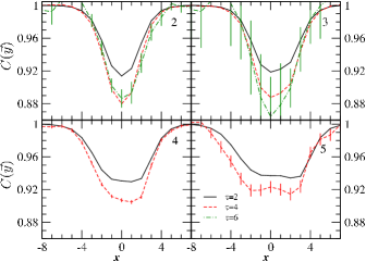
Figure 34: Value of $C(x,0,0)$ for various Y-shape sources of Table 1 where the Euclidean time dependence of the vacuum-action suppression can be examined. Here, $x$ is along the long direction of the quark plane ($z=0$) and with $y=0$ the centre of the node is encountered. Results are for the 30-sweep smeared sources.

As the curves of Fig. 34 pass directly through the centre of the node and the flux-tube to the right of the node, the amplitude of the relative vacuum-action suppression, $A$, may be simply read off the plot. While there is substantial enhancement of $A$ in going from $\tau=2$ to 4, the value for $A$ saturates at $\tau=6$.

Hence, the effect of further Euclidean time evolution is to enhance the amplitude, $A$, of the relative vacuum-action expulsion. The enhancement factor is uniform over the various separations at 1.3(1). Applying this correction to our earlier results for the seventh quark separation where the node and flux tube are well separated, we find $A=0.081(7)$ and 0.072(6) for the node and flux-tube respectively.

VIII CONCLUSIONS

We have studied extensively correlations of the vacuum-action density with Wilson loops describing the three-quark static-baryon system as defined in Eq. (3). A high-statistics approach based on the translational and rotational symmetry of the four-dimensional lattice volume is adopted to avoid the need for gauge-dependent smoothing techniques.

The correlations indicate that the vacuum-action density is suppressed in the interior and surrounding volume in accord with previous findings in the quark-antiquark case. “Flux tubes” represent the expulsion or suppression of vacuum gluon-field fluctuations.

For small quark separations, the ground state is accessed easily through the use of spatially-smeared APE links in the construction of the source and sink of the three-quark system. As illustrated in Fig. 8, the vacuum-action suppression is quite spherical just outside the quark positions, and is strongest in the very centre of the three-quark system. As such, there is no evidence of the formation of a $\Delta$-shape flux-tube (empty triangle) distribution.

As the quarks become more separated the vacuum expulsion takes the shape of a solid or filled triangle. We conclude that at small quark separations i.e. for $\langle r_{s}\rangle\leq 0.5$ fm Y-shape flux-tube formation does not occur. As illustrated in Figs. 8, 8 and 9 a localized junction of flux tubes is not observed.

For quark separations where the quarks are more than 0.5 fm from the system centre, flux-tube formation is observed, in support of Refs. Takahashi:2002bw ; Alexandrou:2002sn ; deForcrand:2005vv ; Ichie:2002mi . Here, the action distribution shows some dependence on the source due to the limited Euclidean time evolution that is possible. Through a study of 8 T and Y shapes and 11 L shapes of varying sizes, we are able to quantitatively demonstrate that the observed potential is a linear function of the length of string required to connect the quark positions to the observed position of the node connecting the flux tubes. This is illustrated in Figs. 19 and 27 for the 10- and 30-sweep sources respectively. As such, the ground state potential at large quark separations is the flux-tube distribution which minimizes this length. In this case the node will be located at the Fermat point.

We have shown that T-shape sources have a flux-tube distribution which relaxes towards a Y-shape distribution as the ground state of the static quark potential is accessed. This is illustrated in Fig. 26 with the corresponding effective potentials presented in Fig. 21. While the formation of a Y-shape flux-tube has been observed before (see Ichie:2002mi for example), to the best of our knowledge this is the first time such a structure has been observed in a gauge invariant manner and observed to emerge from sources that do not have a Y-shape bias.

We have successfully exposed the flux-tube distribution of the ground-state static-quark baryon system at large separations. Figures 24 and 26 provide the best illustrations of this flux-tube distribution. Animations for a variety of quark separations are available on the web webAnim .

Finally the characteristic sizes of the flux-tube and node have been quantified. We find the ground state flux-tube radius to be 0.38(3) fm with vacuum-field fluctuations suppressed by 7.2(6)%. The node connecting the flux tubes is 24(9)% larger at 0.47(2) fm with a 15(3)% larger suppression of the vacuum action at 8.1(7)%.

- (1) J. Flower, Nucl. Phys. B 289, 484 (1987).
- (2) T. T. Takahashi, H. Matsufuru, Y. Nemoto and H. Suganuma, Phys. Rev. Lett. 86, 18 (2001). T. T. Takahashi, H. Suganuma, Y. Nemoto and H. Matsufuru, Phys. Rev. D 65, 114509 (2002) [arXiv:hep-lat/0204011].
- (3) C. Alexandrou, P. De Forcrand and A. Tsapalis, Phys. Rev. D 65, 054503 (2002) [arXiv:hep-lat/0107006].
- (4) C. Alexandrou, P. de Forcrand and O. Jahn, Nucl. Phys. Proc. Suppl. 119, 667 (2003) [arXiv:hep-lat/0209062].
- (5) Ph. de Forcrand and O. Jahn, Nucl. Phys. A 755, 475 (2005) [arXiv:hep-ph/0502039].
- (6) H. Ichie, V. Bornyakov, T. Streuer and G. Schierholz, Nucl. Phys. Proc. Suppl. 119, 751 (2003) [arXiv:hep-lat/0212024]. V. G. Bornyakov et al. [DIK Collaboration], Phys. Rev. D 70, 054506 (2004) [arXiv:hep-lat/0401026].
- (7) J. M. Cornwall, Phys. Rev. D 69, 065013 (2004) [arXiv:hep-th/0305101].
- (8) F. Okiharu and R. M. Woloshyn, Nucl. Phys. Proc. Suppl. 129, 745 (2004) [arXiv:hep-lat/0310007].
- (9) F. Bissey et al., Nucl. Phys. Proc. Suppl. 141, 22 (2005) [arXiv:hep-lat/0501004].
- (10) R. Sommer, Nucl. Phys. B 291, 673 (1987).
- (11) G. S. Bali, K. Schilling and C. Schlichter, Phys. Rev. D 51, 5165 (1995) [arXiv:hep-lat/9409005].
- (12) R. W. Haymaker, V. Singh, Y. C. Peng and J. Wosiek, Phys. Rev. D 53, 389 (1996) [arXiv:hep-lat/9406021].
- (13) M. Falcioni, M. L. Paciello, G. Parisi and B. Taglienti, Nucl. Phys. B 251, 624 (1985). M. Albanese et al. [APE Collaboration], Phys. Lett. B 192, 163 (1987).
- (14) S. O. Bilson-Thompson, D. B. Leinweber and A. G. Williams, Annals Phys. 304, 1 (2003) [hep-lat/0203008].
- (15) M. Luscher and P. Weisz, Commun. Math. Phys. 97, 59 (1985) [Erratum-ibid. 98, 433 (1985)].
- (16) I. Montvay and G. Münster, “Quantum Fields on a Lattice” (Cambridge, 1994) 389.
- (17) W. H. Press, B. P. Flannery, S. A. Teukolsky and W. T. Vetterling, ”Numerical Recipes in C” (Cambridge University Press, 1992), 681 and references therein.
- (18) www.physics.adelaide.edu.au/theory/staff/leinweber/ VisualQCD/Nobel/