Abstract

We consider the lattice realization of the Standard Model with an additional $Z_{6}$ symmetry. Numerical simulations were performed on the asymmetric lattice, which corresponds to the finite temperature theory. Our choice of parameters corresponds to large Higgs masses ($M_{H}>90$ Gev). The phase diagram was investigated and has been found to be different from that of the usual lattice realization of the Standard Model. It has been found, that the confinement-deconfinement phase transition lines for the $SU(2)$ and $SU(3)$ fields coincide. The transition line between Higgs and symmetric deconfinement parts of the phase diagram and the confinement-deconfinement transition line meet in a triple point. The transition between Higgs and symmetric parts of the phase diagram corresponds to the finite temperature electroweak transition/crossover. We see for the first time evidence that Nambu monopoles are condensed at $T>T_{c}$ while at $T<T_{c}$ their condensate vanishes.

Owing to the present triviality bound the perturbation expansion in the electroweak sector of the Standard Model is considered to work perfectly at the energies of the electroweak scale $M_{Z}$ for Higgs masses up to $1$ Tev [1]. However, it was shown [2], that the finite temperature perturbation expansion breaks down at the temperatures above the electroweak transition/crossover already for Higgs masses above about $60$ GeV. Therefore the present lower bound on the Higgs mass, $M_{H}>114$ GeV, requires the use of nonperturbative techniques while investigating electroweak physics at high temperature. Thus our understanding of electroweak physics, which is based mainly on perturbation theory could be changed drastically at temperatures close to and above the electroweak transition/crossover.

It was shown recently [3, 4, 5] that there is a hidden $Z_{6}$ symmetry in the Higgs and fermion sectors of the Standard Model. The Standard Model on the lattice can be defined in such a way, that the whole model is $Z_{6}$ invariant. The resulting model has the same perturbation expansion as the usual lattice realization of the Standard Model, which does not respect the $Z_{6}$ symmetry. On the other hand, it was argued, that nonperturbatively those two lattice models may represent different physics due to their different symmetry properties. In particular, it was supposed, that these two models may describe the physics at temperatures close to the electroweak crossover in different ways.

In this paper we report results of our investigation of the $Z_{6}$ symmetric lattice version of the Standard Model at finite temperature. We considered the model in the London limit, i.e. with infinite bare Higgs mass. This does not mean, however, that the renormalized mass of the Higgs boson is infinite[6].

The phase diagram of our lattice model (Fig. $1$) differs drastically from that of the usual lattice realization of the Standard Model. Namely, in the latter only one phase is present, the phase transition lines degenerate and become crossover lines[7]. Our lattice model clearly contains three parts. The first one (I) is the confinement phase, where the $SU(3)$ fields confine quarks, and confinement-like forces are observed between the leptons. In the next one (II) there are no confinement-like forces at all but the line-like objects which arise in the unitary gauge are found to be condensed. We identify these objects with quantum generalization of the well-known classical Nambu monopole configurations[8]. The last part of the phase diagram (III) corresponds to the low temperature physics, where the Higgs field is condensed. In this part of the phase diagram Nambu monopoles are not condensed and their density is dropping rapidly when moving away from the transition line. Further we refer to both parts II and III of the diagram as to phases, taking in mind, however, that the transition line between them could be actually a crossover line.

The increase of temperature corresponds to a shift from phase III to phase II. The physical temperature is expressed here as $T=\frac{1}{aN_{T}}$, where $N_{T}$ is the time extent of the lattice while $a$ is the lattice spacing, which depends on the values of the coupling constants. We denote the value of temperature at the transition point as $T_{c}$. Here the monopole condensate plays the role of an order parameter. We do not observe a vanishing of the Nambu monopole condensate in phase III with increasing lattice size. This result leads us to suggest the hypothesis, that those monopoles survive and are condensed in the continuum theory at $T>T_{c}$. This is in accordance with the supposition which was made in the framework of the $SU(2)$ Higgs model in [11] . It was argued in [7] that in the usual definition of the lattice Standard Model the electroweak transition is actually a crossover at the allowed values of the Higgs mass. This has led to the conclusion that the baryon asymmetry could not be produced during the electroweak phase transition, as was suggested in [12]. Our investigation shows, however, that the vacuum structure below and above the transition is different. Therefore, we do not exclude that there is a phase transition of a high order at $T=T_{c}$, where the condensate of electromagnetic monopoles vanishes. Although the high order phase transitions are not well understood, they are known to exist in some lattice and statistical systems [13]. The situation may also be similar to that of the $3D$ Compact $U(1)$ Lattice Higgs Model [14], where the phase boundary consists of a line of first-order phase transitions at small Higgs self-coupling, ending at a critical point. The phase boundary then continues as a Kertesz line across which thermodynamic quantities are nonsingular. It is worth mentioning, that within the $3D$ $SU(2)$ Higgs model [15] it was found that the Z-vortices percolate at $T>T_{c}$ while at $T<T_{c}$ they do not. For this reason in Ref. [15] this transition was called the “percolation transition”. It is also in accordance with our observations, as in $4D$ Z-vortices are known to terminate at Nambu monopoles.

We consider here the lattice model described in [5]. We use asymmetric lattices with time extents $2$ and $4$ and of space sizes from $8^{3}$ up to $24^{3}$. With the definitions of [5] the pure gauge part of the action has the form

$$S_{g} = \beta\sum_{\rm plaquettes}\{2(1-\mbox{${\small\frac{1}{2}}$}{\rm Tr}\,U_{p}\cos\theta_{p})+$$ (1)

$$+\;(1-\cos 2\theta_{p})$$

$$+\;6[1-\mbox{${\small\frac{1}{6}}$}{\rm ReTr}\,\Gamma_{p}{\rm Tr}\,U_{p}{\rm exp}(i\theta_{p}/3)]$$

$$+\;3[1-\mbox{${\small\frac{1}{3}}$}{\rm ReTr}\,\Gamma_{p}{\rm exp}(-2i\theta_{p}/3)]$$

$$+\;3[1-\mbox{${\small\frac{1}{3}}$}{\rm ReTr}\,\Gamma_{p}{\rm exp}(4i\theta_{p}/3)]\},$$

where the sum runs over the elementary plaquettes of the lattice, and

$$\Gamma\in SU(3),\quad U\in SU(2),\quad e^{i\theta}\in U(1).$$ (2)

Each term of the action, Eq. (1), corresponds to a parallel transporter along the boundary $\partial p$ of a plaquette $p$.

The action for the scalar field is considered in its simplest form [4] in the London limit, i.e., in the limit of infinite bare Higgs mass. After fixing the unitary gauge we obtain:

$$S_{H} = \gamma\sum_{xy}[1-Re(U^{11}_{xy}e^{i\theta_{xy}})].$$ (3)

Here $\gamma=v^{2}$, where $v$ is the bare scalar field vacuum average. We consider our model in quenched approximation, i.e., we neglect the effect of virtual fermion loops. Thus the whole action of the model is $S=S_{g}+S_{H}$.

It is worth mentioning, that the action of the form (1) actually appears as a low energy approximation of the $SU(5)$ GUT[3]. Therefore, the bare coupling $\beta$ (which is the same for all terms of the action) could be considered at the GUT scale. Then, owing to the renormalization group equations, the renormalized gauge couplings at the electroweak scale $M_{Z}$ come close to the experimental ones and coincide with them up to a few percents. Actually, their change is of logarithmic form and is very slow. The physical scale (i.e. the value of the lattice spacing in physical units) should be determined using a measurement of the zero-temperature Z-boson mass in lattice units. We did not perform extensive calculation of $M_{Z}$ in our model within the considered ranges of bare couplings. However, our measurements of correlators in the vector channel allow us to evaluate the lattice spacing in the considered region of phase III ($\beta\in(0.6,0.8)$, $\gamma\in(1.0,1.5)$) to be $(130\pm 40\,{\rm GeV})^{-1}$.

The renormalized $\alpha_{s}$ (which stands for the strong interaction of quarks) in our model can be calculated using certain correlators of colored fields and should be expressed as a function of bare couplings. In principle, if we start from the theory at the GUT scale, such a calculation must give a reasonable result. However, due to the technical problems in lattice simulations, we expect direct calculations at the Electroweak scale would give unphysically small values of $\alpha_{s}(M_{Z})$. This means that at the energies of the order of $100$ GeV color fields in our lattice model appear to be suppressed. Thus we consider their influence on the Electroweak dynamics only qualitatively. However, if such an influence (which is due to the specific $Z_{6}$ invariant terms in the action) is found, it is reasonable to expect that it also should take place for the realistic case of unsuppressed colored fields.

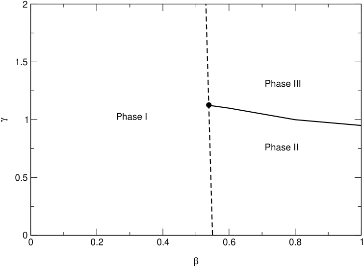
Figure 1: The phase diagram of the model in the $(\beta,\gamma)$-plane for the time extent $N_{T}=2$.

In general all the renormalized gauge couplings should be calculated using static quark and lepton potentials. Then the lines of constant physics (LCP) in the space of bare parameters (including time extent of the lattice) are defined as the lines, where the zero-temperature renormalized couplings and the temperature in physical units are constant[6, 7]. In the present paper we do not consider LCP, which is needed for a proper investigation of approaching continuum physics. The consideration of LCP is also necessary for determining the correspondence between the phase diagram in the $\beta$ - $\gamma$ plane and the conventional phase diagram in the $T-M_{H}$ plane. However, we can understand the emergence of temperature in the phase diagram represented in the Fig. 1 using naive expressions for the lattice spacing and the Z-boson mass. Namely, in phase III at tree level $M_{Z}=g_{z}v/2$ in lattice units. Here, $g_{z}=g/{\rm cos}\,\theta_{W}$, $8\beta=\frac{4}{g^{2}}$, and ${\rm cos}^{2}\,\theta_{W}=\frac{5}{8}$. Therefore $M_{Z}\sim\sqrt{\frac{\gamma}{5\beta}}$. Next, the lattice spacing in physical units is equal to $a=M_{Z}/M^{\rm phys}_{Z}$, where $M^{\rm phys}_{Z}$ is about $90$ GeV. Therefore, say, at $\beta=0.6$, $\gamma=1.5$ the naive tree level estimate for the lattice spacing is $a\sim(130\,{\rm GeV})^{-1}$, while at $\beta=0.8$, $\gamma=1.0$ it is $a\sim(180\,{\rm GeV})^{-1}$. Finally, the temperature is estimated as $T=\frac{1}{N_{T}a}\sim\sqrt{\frac{5\beta}{\gamma N_{T}^{2}}}\,90\,{\rm GeV}$. Although the last expression is to be modified using the lattice renormalization group equations, it shows, that, in general, temperature is increased with an increase of $\beta$ and a decrease of $\gamma$ and $N_{T}$.

Physically interesting values of the coupling constants could be evaluated following the naive estimates considered above. In our model the bare electromagnetic charge is $e^{2}=g^{2}{\rm sin}^{2}\,\theta_{W}=\frac{3}{16\beta}$; the experimental value is $\frac{e^{2}(M_{Z})}{4\pi}\sim\frac{1}{128}$. Thus $\beta\sim\frac{6}{\pi}\sim 1.9$. Our estimate for the critical $\gamma$ at $\beta=1.9$ is $\gamma_{c}\sim 0.9$. Therefore, the critical temperature could be estimated as $T_{c}\sim 150$ GeV. Of course, this is a very rough estimate and it should be improved using direct lattice methods. For technical reasons we did not perform extensive numerical simulations in the vicinity of $\beta\sim 1.9$. Instead we investigated the region $\beta\in(0.6,0.8)$ of phase III. This means that our results at the present moment should be considered as qualitative only.

The following variables are considered as creating a $Z$ boson and a $W$ boson, respectively:

$$Z_{xy} = Z^{\mu}_{x}\;={\rm sin}\,[{\rm Arg}U_{xy}^{11}+\theta_{xy}],$$

$$W_{xy} = W^{\mu}_{x}\,=\,U_{xy}^{12}e^{i\theta_{xy}}.$$ (4)

Here, $\mu$ represents the direction $(xy)$.

After fixing the unitary gauge the electromagnetic $U(1)$ symmetry remains:

$$U_{xy} \rightarrow g^{\dagger}_{x}U_{xy}g_{y},$$

$$\theta_{xy} \rightarrow \theta_{xy}-\alpha_{y}/2+\alpha_{x}/2,$$ (5)

where $g_{x}={\rm diag}(e^{i\alpha_{x}/2},e^{-i\alpha_{x}/2})$.

In the unitary gauge there is also a $U(1)$ lattice gauge field, which is defined as

$$A_{xy}=A^{\mu}_{x}\;=\,[-{\rm Arg}U_{xy}^{11}+\theta_{xy}]\,{\rm mod}\,2\pi,$$ (6)

The fields $A$, $Z$, and $W$ transform as follows:

$$A_{xy} \rightarrow A_{xy}-\alpha_{y}+\alpha_{x},$$

$$Z_{xy} \rightarrow Z_{xy},$$

$$W_{xy} \rightarrow W_{xy}e^{-i\alpha_{x}}.$$ (7)

It should be mentioned that the field $A$ cannot be treated as a usual electromagnetic field as the set of variables $A$, $Z$, and $W$ do not diagonalize the kinetic part of the pure gauge action (1) in its naive continuum limit. In our lattice model the electromagnetic field $A_{\rm em}$ should be defined as

$$A_{\rm em}=A+Z^{\prime}-2\,{\rm sin}^{2}\,\theta_{W}Z^{\prime},$$ (8)

where $Z^{\prime}=[{\rm Arg}U_{xy}^{11}+\theta_{xy}]{\rm mod}2\pi$. The naive value of the Weinberg angle corresponds to ${\rm sin}^{2}\,\theta_{W}=\frac{3}{8}$. However, the renormalized Weinberg angle is to be calculated through the ratio of the lattice masses: ${\rm cos}\,\theta_{W}=\frac{M_{W}}{M_{Z}}$.

In order to evaluate the zero temperature masses of the $Z$-boson and Higgs boson we use the correlators:

$$\langle\sum_{\mu}Z^{\mu}_{x}Z^{\mu}_{y}\rangle \sim \frac{1}{|x-y|^{2}}e^{-M_{Z}|x-y|}$$

$$\langle\langle H_{x}H_{y}\rangle\rangle = \langle H_{x}H_{y}\rangle-\langle H\rangle^{2}\sim\frac{1}{|x-y|^{2}}e^{-M_{H}|x-y|},$$ (9)

where $H_{x}=\sum_{y}|W_{xy}|^{2}$ or $H_{x}=\sum_{y}Z^{2}_{xy}$.

The position of the transition lines on the phase diagram of the finite temperature model almost coincide with that of the lines on the phase diagram of the zero temperature model[5]. The only difference is that the transition line between phases II and III is shifted to higher values of $\gamma$. Our statistics does not allow us to perform a precise calculation of the values of $M_{H}$ and $M_{Z}$. Therefore we have made a very rough estimate of their ratio. Namely, in phase III of the zero temperature model (on the lattice $16^{4}$) for the considered values of the couplings ($\beta\in(0.5,0.8)$, and $\gamma$ up to $1.5$) our estimate is $M_{H}/M_{Z}\sim 2.5\pm 0.5$. This is in qualitative agreement with the predictions made within the $SU(2)$ Higgs model considered in the London limit [6]. Thus in our model the estimate for the Higgs mass could be $M_{H}\sim 230\pm 50$ GeV. However, as it was mentioned above, the lattice spacing in the considered part of the phase diagram is estimated to be $(130\pm 40\,{\rm GeV})^{-1}$. In lattice theory the inverse lattice spacing plays the role of an ultraviolet cutoff. In general, quantum field theory does not work at energies higher than the ultraviolet cutoff. Therefore, we feel it necessary to weaken our estimate for $M_{H}$. Namely, we evaluate it as $M_{H}>90$ GeV.

To understand the dynamics of external charged particles, we consider the Polyakov lines defined on the asymmetric lattice in the fermion representations listed in the table in [5]:

$${\cal P}^{\rm L}_{\rm lept} = \langle{\rm Re}{\rm Tr}\,\Pi_{(xy)\in l}U_{xy}e^{-i\theta_{xy}}\rangle,$$

$${\cal P}^{\rm R}_{\rm lept} = \langle{\rm Re}\Pi_{(xy)\in l}\,e^{-2i\theta_{xy}}\rangle,$$

$${\cal P}^{\rm L}_{{\rm quarks}} = \langle{\rm Re}\Pi_{(xy)\in l}\,\Gamma_{xy}\,U_{xy}\,e^{\frac{i}{3}\theta_{xy}}\rangle,$$

$${\cal P}^{\rm R}_{{\rm down}\,{\rm quarks}} = \langle{\rm Re}\Pi_{(xy)\in l}\,\Gamma_{xy}\,e^{-\frac{2i}{3}\theta_{xy}}\rangle,$$

$${\cal P}^{\rm R}_{{\rm up}\,{\rm quarks}} = \langle{\rm Re}\Pi_{(xy)\in l}\,\Gamma_{xy}\,e^{\frac{4i}{3}\theta_{xy}}\rangle.$$ (10)

Here $l$ denotes a line on the lattice in the time direction, which is closed due to the periodic boundary conditions.

It is found that to the left of the vertical line of the phase diagram all Poliakov lines vanish while to the right of this line all of them increase rapidly (Fig. $2$).

In order to extract physical information from the $SU(3)$ fields themselves in a particulary simple way we use the so-called indirect Maximal Center Projection (see, for example, [16, 17]).

We investigated several types of monopoles. The monopoles, which carry information about colored fields are extracted from the composite fields $C^{i}$ (for their definition see [5]) constructed of the $SU(2)$ and $U(1)$ fields and of the center vortices appearing in the Maximal Center Projection of the color group:

$$j_{C^{i}}=\frac{1}{2\pi}{}^{*}d([dC^{i}]{\rm mod}2\pi).$$ (11)

(Here we used the notations of differential forms on the lattice. For a definition of those notations see, for example,  [18].) Pure $U(1)$ monopoles, corresponding to the second term in (1), are extracted in the same way from $2\theta$: $j_{2\theta}=\frac{1}{2\pi}{}^{*}d([d2\theta]{\rm mod}2\pi)$. We refer to them as hypercharge monopoles.

The electromagnetic monopoles must be related to the field $A_{\rm em}$. However, $A_{\rm em}$ itself is not a usual lattice $U(1)$ field that should be periodic with the period $2\pi$. Instead $A_{\rm em}$ is constructed of the two $U(1)$ variables: $A$ and $Z^{\prime}$. Therefore, the electromagnetic monopoles should be constructed of either $A$ or $Z^{\prime}$ fields, or, possibly both of them. Therefore, we denote these monopoles by $j_{A}=\frac{1}{2\pi}{}^{*}d([dA]{\rm mod}2\pi)$ and $j_{Z}=\frac{1}{2\pi}{}^{*}d([dZ^{\prime}]{\rm mod}2\pi)$.

The worldsheet of the quantum $Z$-string may be defined as $\sigma_{Z}=\frac{1}{2\pi}\{[dZ^{\prime}]\,{\rm mod}2\pi-dZ^{\prime}\}$. This is actually a Nielsen-Olesen string embedded in the Standard Model.

On the classical level the singularity of the hypercharge field $2\theta=[A+Z^{\prime}]{\rm mod}2\pi$ is suppressed by the $U(1)$ pure gauge field action. Therefore, one would expect that $j_{Z}=-j_{A}$. This situation corresponds to the appearance of the quantum Nambu monopole with the worldline $j_{A}$. From (8) it follows that its magnetic charge is proportional to $4\pi{\rm sin}^{2}\theta_{W}$ as it should [8].

In lattice quantum theory, however, the singularities of the hypercharge field may appear in the form of the corresponding monopoles. This situation corresponds to the appearance of $j_{2\theta}$. Then in the absence of a $Z$-string the magnetic charge of such configurations appear to be proportional to $2\pi$. This case of the magnetic monopole for even $j_{A}$ seems to be corresponding to a Cho-Maison monopole or dyon [9] .

Thus, we arrive at the following two possibilities:

1. In the absence of $j_{2\theta}$ the A-monopoles $j_{A}$ represent Nambu monopoles with the magnetic charge $4\pi{\rm sin}^{2}\theta_{W}$.

2. If $j_{2\theta}\neq 0$ the A-monopoles may represent another type of monopoles with the magnetic charge $2\pi$. Such a monopole with even $j_{A}$ corresponds to Cho-Maison monopole or dyon.

The density of the monopoles is defined as follows:

$$\rho=\left\langle\frac{\sum_{\rm links}|j_{\rm link}|}{4L^{4}}\right\rangle,$$ (12)

where $L$ is the lattice size.

It is found that the densities of the color and hypercharge monopoles decrease rapidly to the right of the vertical line in the phase diagram and drop to zero soon after the phase transition. This, together with the behavior of the Polyakov lines allows us to identify the vertical line of the phase diagram with the confinement-deconfinement phase transition common for $U(1)$, $SU(2)$, and $SU(3)$ fields. The behavior of such quantities as the overall action and the monopole densities possess hysteresis effects, which allow us to suppose that this phase transition is of the first order. The position of the phase transition is localized using hysteresis of the action and is defined as the point where the mentioned Polyakov lines vanish.

The monopole density $\rho(A)$ constructed of $j_{A}$ is found to be nonzero for all values of the couplings considered within phase II. As the hypercharge monopoles disappear in this phase, we identify here $j_{A}$ with Nambu monopoles. When going to phase III the density decreases and vanishes soon after the transition. In order to investigate the condensation of the electromagnetic monopoles we use the percolation probability $\Pi(A)$. It is the probability that two infinitely distant points are connected by a monopole cluster (for more details of the definition see, for example, [17]). We found that this probability is an order parameter, which feels the transition (Fig. $3$). We define the position of the transition using maximum of the susceptibility $\chi=\langle H^{2}\rangle-\langle H\rangle^{2}$. It coincides with the point, where the percolation probability vanishes. At the same time there is no abrupt change of the action on the transition line. The correlation lengths extracted from the space-like correlators (9) on the asymmetric lattices do not increase when approaching the transition line between the phases II and III. Let us remind here again that in the conventional lattice Standard Model the similar transition is found to be a crossover [7]. However, in [15] it was found that the $Z$-strings are condensed at high temperatures in the $3D$ $SU(2)$ Higgs model, while at low temperatures they are not. For this reason this transition was called in [15] “percolation transition”. We did not investigated in detail the transition between phases II and III in our model. Therefore, we cannot draw a definite conclusion as to the nature of this transition. However, the percolation properties of Nambu monopoles show that the vacuum structure at $T>T_{c}$ differs from the vacuum structure at $T<T_{c}$. Therefore, we do not exclude, that this is actually a phase transition of a high order.

Investigation of different sizes of the lattices (from $8^{3}\times 2$ up to $24^{3}\times 4$) shows that neither the density nor the percolation of Nambu monopoles decrease with increasing lattice size for the values of the couplings considered (up to $\beta=2.0$) in phase II of the model. Therefore we suppose that those monopoles survive in the continuum theory like the Abelian projected monopoles of pure nonabelian gauge models.

The properties of quantum Cho-Maison monopoles are sufficiently different from those of the Nambu monopoles as the hypercharge monopole density within the physical phases II and III decrease rapidly when moving away from the vertical phase transition line. For this reason we do not exclude that Cho-Maison monopoles may completely disappear in the continuum theory.

To conclude, we have considered the $Z_{6}$ symmetric lattice version of the Standard Model on the lattice at finite temperature. We must mention, that the considered lattice model is obtained as a result of several simplifications. First of all, we neglect dynamical fermions. Next, we froze radial fluctuations of the scalar field. Finally, our choice of gauge couplings corresponds to the $SU(5)$ unified theory. As a result, strictly speaking, the model may describe color fields quantitatively only at the energies close to the GUT scale. However, we expect that even at the Electroweak scale this model may describe qualitatively the influence of the emergence of $Z_{6}$ symmetry in the lattice action on the phase diagram. We must remind here, that without $Z_{6}$ symmetry there is no influence of color fields on the Electroweak dynamics at all (if one neglects fermion loops).

We have found that at least the lattice model itself differs from the usual realization of the Standard Model on the lattice. Namely, there is a confinement-deconfinement phase transition line common to $SU(2)$, $SU(3)$, and $U(1)$ fields. This line and the line of the transition which corresponds to the finite temperature electroweak transition/crossover, meet together in a triple point. However, we do not consider properly the limit of vanishing lattice spacing. Therefore at the present moment we do not exclude that the mentioned new features of the $Z_{6}$ invariant lattice Standard Model may disappear in the continuum limit.

Nambu monopoles appeared to be condensed at $T>T_{c}$ in our lattice model. We suppose that at $T>T_{c}$ they survive in the continuum theory. Finally, if those monopoles are indeed present at $T>T_{c}$ it would be natural to suppose, that they may appear at low temperatures in the form of ordinary particles . It is worth mentioning, that although we started from the $Z_{6}$ invariant form of lattice Standard Model, our prediction of the behavior of quantum Nambu monopoles could be unchanged even without taking care of $Z_{6}$ symmetry. This should be, of course, the subject of another research.

We are grateful to F.V. Gubarev, M.N.Chernodub, E.M. Ilgenfritz, and D. Boer for useful discussions. A.I.V. and M.A.Z. kindly acknowledge the hospitality of the Department of Physics and Astronomy of the Vrije Universiteit, where part of this work was done. This work was partly supported by the Netherlands Organisation for Scientific Research, by RFBR grants 06-02-16309, 05-02-16306, and 04-02-16079, RFBR-DFG grant 06-02-04010, by Federal Program of the Russian Ministry of Industry, Science and Technology No 40.052.1.1.1112, by Grant for leading scientific schools 843.2006.2.

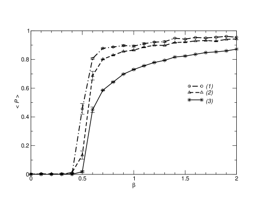
Figure 2: The expectation value of Polyakov lines as a function of $\beta$ for a fixed value $\gamma=0.5$. (1) corresponds to ${\cal P}^{\rm R}_{\rm lept}$; (2) corresponds to ${\cal P}^{\rm L}_{\rm lept}$; (3) corresponds to ${\cal P}^{\rm L}_{\rm quarks}$.

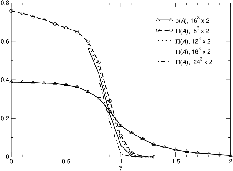
Figure 3: The density $\rho(A)$ of Nambu monopoles and the percolation probability $\Pi(A)$ as a function of $\gamma$ for a fixed value $\beta=0.6$.

References

- [1] Bohdan Grzadkowski, Jose Wudka, IFT-31/2001, UCRHEP-T321, Acta Phys. Polon. B 32 (2001) 3769-3782
-
[2]
Peter Arnold and Olivier Espinosa, Phys. Rev. D 47 (1993) 3546.
Z. Fodor and A. Hebecker, Nucl. Phys. B 432 (1994) 127.
W. Buchmuller, Z. Fodor, and A. Hebecker, Nucl. Phys. B 447 (1995) 317.
- [3] B.L.G. Bakker, A.I. Veselov, and M.A. Zubkov, Phys. Lett. B 583, 379 (2004);
- [4] B.L.G. Bakker, A.I. Veselov, and M.A. Zubkov, Yad. Fiz. 68, 1045 (2005).
- [5] B.L.G. Bakker, A.I. Veselov, and M.A. Zubkov, Phys. Lett. B 620 (2005) 156-163.
- [6] I. Montvay, Nucl. Phys. B 269, 170 (1986).
- [7] F. Csikor, Z. Fodor, and J. Heitger, Phys. Rev. Lett. 82 (1999) 21-24. M. Gurtler, E.-M. Ilgenfritz, and A. Schiller, Phys. Rev. D 56 (1997) 3888-3895. K. Rummukainen, M. Tsypin, K. Kajantie, M. Laine, and M. Shaposhnikov, Nucl. Phys. B 532 (1998) 283-314. Yasumichi Aoki, Phys. Rev. D 56 (1997) 3860-3865. N. Tetradis, Nucl. Phys. B 488 (1997) 92-140. B. Bunk, Ernst-Michael Ilgenfritz, J. Kripfganz, A. Schiller, BI-TP-92-46, Nucl.Phys.B bf 403, 453 (1993). B. Bunk, Ernst-Michael Ilgenfritz , J. Kripfganz, A. Schiller, BI-TP-92-12, Phys.Lett.B 284, 371 (1992).
- [8] Y. Nambu, Nucl.Phys. B 130, 505 (1977) Ana Achucarro, Tanmay Vachaspati, Phys. Rept. 327, 347 (2000); Phys. Rept. 327, 427 (2000)
- [9] Y. M. Cho, D. Maison, Phys.Lett. B 391, 360 (1997)
- [10] K. Kajantie, M. Laine, K. Rummukainen, and M. Shaposhnikov, Phys. Rev. Lett. 77 (1996) 2887-2890.
- [11] M.N. Chernodub, JETP Lett. 66, 605 (1997)
- [12] V.A.Kuzmin, V.A.Rubakov, and M.E.Shaposhnikov, Phys. Lett. B 155, 36 (1985)
- [13] W. Janke, D.A. Johnston, R. Kenna, XXIIIrd Int. Symp. Latt. Field Theory, Proceedings of Science (LAT2005) 244, hep-lat/0512022
- [14] Sandro Wenzel, Elmar Bittner, Wolfhard Janke, Adriaan M.J. Schakel, A. Schiller, Phys. Rev. Lett. 95, 051601 (2005)
-
[15]
M.N. Chernodub, F.V. Gubarev, E.M. Ilgenfritz, and A. Schiller,
Phys. Lett. B 434, 83 (1998);
M.N. Chernodub, F.V. Gubarev, E.M. Ilgenfritz, and A. Schiller, Phys. Lett. B 443, 244 (1998). - [16] J. Greensite, Prog. Part. Nucl. Phys. 51 (2003) 1
- [17] B.L.G. Bakker, A.I. Veselov, and M.A. Zubkov, Phys. Lett. B 471 (1999) 214
- [18] M.I. Polikarpov, U.J. Wiese, and M.A. Zubkov, Phys. Lett. B 309, 133 (1993).