A gauge invariant cluster algorithm for the Ising spin glass

Abstract

The frustrated Ising model in two dimensions is revisited. The frustration is quantified in terms of the number of non-trivial plaquettes which is invariant under the Nishimori gauge symmetry. The exact ground state energy is calculated using Edmond’s algorithm. A novel cluster algorithm is designed which treats gauge equivalent spin glasses on equal footing and allows for efficient simulations near criticality. As a first application, the specific heat near criticality is investigated.

Spin glasses Binder86 are magnetic materials in which the magnetic moments are subject to ferromagnetic or anti-ferromagnetic interactions, depending on the position of the moments within the sample. The system is frustrated in the sense that the arrangement of spins which minimizes the total energy cannot be determined by considering a local set of spins. Stated differently, the change of a single spin might cause a reordering of many spins when the system relaxes towards a new minimum of energy Alava98 . Spin glasses undergo a freezing transition to a state where the order is represented by clusters of spins with mixed orientations. The relaxation times towards equilibrium are typically very large, which impedes efficient simulations.

Many efforts have been undertaken to explore equilibrium properties of spin glasses by means of Monte Carlo simulations Binder79 ; Binder80 ; Young82 ; Ogielski85 ; Huse85 ; Rieger96 ; Matsubara97 ; Shirakura97 . Thereby, many insights have been obtained from the most simple case of the 2d Ising model on a square lattice. For the discrete model, the bond interactions take values $J_{\ell}=\pm 1$ at random, and the model is characterized by the the probability $p$ of finding an anti-ferromagnetic interaction, $J_{\ell}=-1$, at a given bond. At present, the existence of a spin glass transition in these models at $T_{c}\neq 0$ is still under debate.

As first noticed by Bieche et al. Bieche80 and further elaborated by Nishimori Nishimori1981 ; Nishimori1983 , the Ising model with random distribution of anti-ferromagnetic bonds has a hidden $Z_{2}$ gauge symmetry. As discussed below, this symmetry implies that gauge invariant observables such as the thermal energy or the specific heat are unchanged by a certain redistribution of the anti-ferromagnetic bonds (which may also change their number considerably). By exploiting this invariance, Nishimori was able to obtain exact results for special values of the parameters $p$ and $T$ Nishimori1981 ; Nishimori1983 .

The generic difficulty in simulating spin systems is that the auto-correlation time $\tau$ increases rapidly with the physical correlation length $\xi$ of the system, $\tau\propto\xi^{z}$, where $z$ is the dynamical critical exponent. For all local update algorithms, $z$ is as large as $2$. This is particularly problematic at small temperatures, when $\xi$ reaches the extension $L$ of the lattice and the generation of independent configurations in a Markov chain becomes extremely cumbersome. As a consquence, the auto-correlation times must be monitored very carefully or the algorithm might fail to be ergodic. For a pure ferromagnet, the ground state is known explicitly: A state with all spins parallel minimizes the energy. This knowledge of the true ground state can be used to design an efficient algorithm which microcanonically changes clusters of spins with the same orientation. Indeed, the so-called cluster algorithms swendsen87 ; wolff89 largely alleviate the auto-correlation problem: the dynamical critical exponent drops to values $z\approx 0.4$ which renders practical simulations on large lattices feasible.

So far, cluster algorithms for the frustrated Ising model do not exist. This is mainly due to the fact that the true ground state (and hence the structure of the physical clusters) is unknown for a generic distribution of anti-ferromagnetic bonds. In fact, finding the ground state is an NP hard problem in $d\geq 3$. For the special case $d=2$, Edmond’s algorithm Edmonds65a ; Edmonds65b provides a method which computes the exact ground state in polynomial time. This can be used to clearify the structure of the physical clusters in special gauges, which would otherwise be obfuscated by the hidden gauge symmetry.

In this letter, we quantify the amount of frustration in the 2d Ising model in a gauge invariant way by counting the fraction $\rho$ of vortices (non-trivial plaquettes) in a given bond distribution. First, we determine the exact ground state energy as a function of $\rho$ using Edmond’s algorithm. In order to treat the system near criticality, we present a novel cluster update algorithm which proposes clusters in a gauge independent way. The specific heat as a function of the inverse temperature is explicitly evaluated for models with different frustrations, and gauge independence is verified.

The partition function of the frustrated Ising model involves a summation over all spin configurations $\{\sigma_{x}\}$

$$Z\;=\;\sum_{\{\sigma_{x}\}}\;\exp\Bigl{\{}\sum_{\ell=\langle xy\rangle}\beta_{\ell}\;\sigma_{x}\;\sigma_{y}\Bigr{\}}\;,$$ (1)

where the spins located at the sites of the lattice take the values $\sigma_{x}=\pm 1$. The sum in the exponent extends over all bonds $\ell=\langle xy\rangle$ and the coupling constants $\beta_{\ell}$ are chosen positive and equal to $\beta>0$, except for a fraction $\kappa$ of the bonds where the couplings are $(-\beta)$. In the zero temperature limit $\beta\rightarrow\infty$, the anti-ferromagnetic couplings induce frustration.

It was first observed by Nishimori Nishimori1981 ; Nishimori1983 that bond distributions with vastly different values for $\kappa$ may still share the same thermodynamical properties. This is due to a $Z_{2}$ gauge symmetry, which becomes transparent if we introduce link variables $U_{\ell}\;=\;\hbox{sign}(\beta_{\ell})$. With this notation, the thermal energy is given by

$$E(T)\;=\;-\;\Bigl{\langle}\sum_{\ell=\langle xy\rangle}\;\sigma_{x}\,U_{\ell}\,\sigma_{y}\;\Bigr{\rangle}\;.$$ (2)

The partition function, eq. (1), and observables such as the thermal energy, eq. (2), are invariant under the following change of bonds and spin variables:

$$\sigma^{\Omega}(x) = \Omega(x)\;\sigma(x)$$

$$U^{\Omega}_{\langle xy\rangle} = \Omega(x)\;U_{\langle xy\rangle}\;\Omega^{-1}(y)\;,$$ (3)

where the gauge transformation takes values in $Z_{2}$, $\Omega(x)=\pm 1$. In order to characterize the frustration of the model, we introduce the plaquette variable, $P(p)\;=\;\prod_{\ell\in p}U_{\ell}$, constructed from the given bond background. This definition is borrowed from lattice gauge theory, where a non-trivial value $P(p)=-1$ indicates that a $Z_{2}$ vortex intersects the plaquette $p$. Notice that the variable $P(p)$ is invariant under the $Z_{2}$ gauge transformation (3), and the distribution of vortices is thus the proper measure to quantify the frustration of the model.

With a given vortex content, there is still a large number of gauge equivalent bond distributions which share the same physical properties. In particle physics, the bond distribution with the minimal number of anti-ferromagnetic bonds is known as Landau gauge,

$$\sum_{\ell=\langle xy\rangle}\;U^{\Omega}_{\ell}\;\stackrel{{\scriptstyle\Omega}}{{\longrightarrow}}\;\hbox{max}\;.$$ (4)

For this choice of bond distribution, the ground state is always uniform,

$$\sigma_{x}^{\Omega_{L}}\;=\;\sigma_{y}^{\Omega_{L}}\;=\;\hbox{const.}\;\;\forall x,y\;,\;\;\hbox{ (Landau gauge) }.$$ (5)

To see this, we can use eqs. (3) and (4) to express the energy of a given spin configuration $\{\sigma\}$ in a Landau gauge background as

$$E[\sigma] = -\sum_{\ell=\langle xy\rangle}\sigma_{x}\;U_{\ell}^{\Omega_{L}}\;\sigma_{y}=-\sum_{\ell=\langle xy\rangle}U_{\ell}^{\sigma\cdot\Omega_{L}}$$

$$\geq -\sum_{\ell=\langle xy\rangle}U^{\Omega_{L}}_{\ell}=-\sum_{\ell=\langle xy\rangle}\sigma_{x}^{\Omega_{L}}\;U^{\Omega_{L}}_{\ell}\;\sigma_{y}^{\Omega_{L}}=E[\sigma^{\Omega_{L}}]\;,$$

where we used the maximum condition eq. (4) for the inequality and the definition eq. (5) for the uniform ground state.

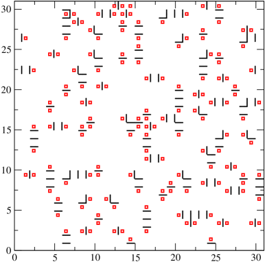
Figure 1: Left panel: $n_{v}=150$ randomly distributed vortices (red squares) on a $30\times 30$ lattice and the corresponding minimal matching with anti-ferromagnetic bonds (black lines). Ground state energy per link: $E_{0}\;=\;-0.837778(1)$. Right panel: ground state energy as function of the density of frustration $\rho$.

Let us consider a particular distribution of anti-ferromagnetic bonds on the lattice. The ground state energy can be obtained as follows: (i) Calculate the position of the vortices on the lattice; (ii) construct the minimal number $N_{A}$ of anti-ferromagnetic links which are compatible with the given vortices, (iii) obtain the gauge transformation $\Omega_{x}$ which casts the original bond distribution to the one obtained in step (ii). As shown above, the gound state in the bond distribution (ii) is uniform and its energy can be read off directly,

$$E_{0}\;=\;N_{A}\;-\;2\,N_{\ell},$$ (6)

where $N_{\ell}\;=\;d\,L^{d}$ is the total number of bonds on the lattice. Transforming back to the initial bond distribution, the energy $E_{0}$ remains unchanged while the ground state becomes $\sigma^{0}_{x}=\Omega_{x}^{-1}$. The practical difficulty in this algorithm lies in step (ii) which is NP hard except for the case $d=2$, where Edmond’s algorithm Edmonds65a ; Edmonds65b provides an efficient solution in polynomial time Bieche80 . Figure 1 shows a random distribution of $n_{v}=150$ vortices and the corresponding minimal number of frustrated bonds, which were obtained with Edmond’s algorithm. Also shown is the ground state energy as function of the vortex density $\rho=n_{v}/L^{2}$. The data comprise an average over 100 vortex distributions for each value of $\rho$.

In the following, we will construct a cluster algorithm which strongly reduces auto-correlations near criticality and which, in addition, is gauge invariant. For this purpose, we follow the derivation of the Swendsen-Wang cluster algorithm swendsen87 , but firstly divide the bonds into those with ferromagnetic and anti-ferromagnetic couplings, respectively. For the ferromagnetic bonds, we make use of the identity

$$\exp\{\beta\;\sigma_{x}\;\sigma_{y}\}\;=\;e^{\beta}\;\left[\left(1-q\right)\;+\;q\;\delta_{\sigma_{x}\sigma_{y}}\right]\;,$$ (7)

with $q=1-e^{-2\beta}$. A similar expression holds for the anti-ferromagnetic bonds,

$$\exp\{-\beta\;\sigma_{x}\sigma_{y}\}=e^{\beta}\;\left[\left(1-q\right)+q\;(1-\delta_{\sigma_{x}\sigma_{y}})\right]\;.$$ (8)

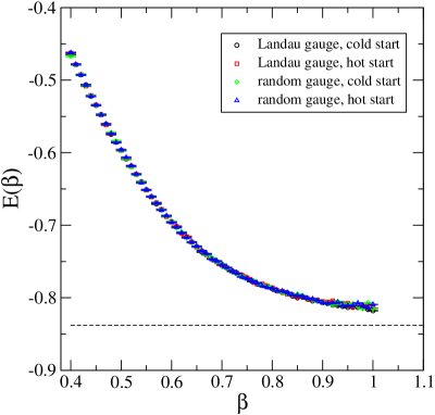
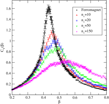
Figure 2: Left panel: Thermal energy as a function of $\beta$ for the configuration depicted in figure 1. Right: Specific heat for a $30\times 30$ lattice with $n_{v}$ randomly chosen vortices.

The partition function can thus be written as

$$Z = e^{N_{\ell}\,\beta}\sum_{\{\sigma_{x}\}}\;\prod_{\ell}\Bigl{\{}\theta(\beta_{\ell})\;\bigl{[}(1-q)\,+\,q\;\delta_{\sigma_{x}\sigma_{y}}\bigr{]}$$

$$+ \theta(-\beta_{\ell})\;\bigl{[}\left(1-q\right)\;+\;q\;(1-\delta_{\sigma_{x}\sigma_{y}})\bigr{]}\Bigr{\}}\;,$$

where $N_{\ell}$ is the total number of bonds on the lattice. The bond activation variable $n\in\{0,1\}$ is introduced via the identity

$$a\;+\;b\;=\;\sum_{n=0}^{1}\Bigl{[}a\;\delta_{n0}\;+\;b\;\delta_{n1}\Bigr{]}\;.$$ (10)

The partition function is now recast to

$$Z=e^{N_{\ell}\,\beta}\;\sum_{\{\sigma_{x}\}}\;\sum_{\{n_{\ell}\}}\;P(\sigma,n)\;,$$ (11)

where

$$P(\sigma,n) = \prod_{\ell=\langle xy\rangle}\biggl{\{}\theta(U_{\ell})\,\Bigl{[}\delta_{n_{\ell}\,0}\,(1-q)\,+\,\delta_{n_{\ell}\,1}\,q\,\delta_{\sigma_{x}\sigma_{y}}\Bigr{]}$$

$$+ \theta(-U_{\ell})\,\Bigl{[}\delta_{n_{\ell}\,0}\,(1-q)\,+\,\delta_{n_{\ell}\,1}\,q\,(1-\delta_{\sigma_{x}\sigma_{y}})\,\Bigr{]}\,\biggr{\}}\;.$$

For the cluster update algorithm we perform subsequent updates of the bond variables $n_{\ell}$ and the spin variables $\sigma_{x}$. Let us first discuss the $n_{\ell}$ update and consider a specific bond $\ell=\langle xy\rangle$. If $\ell$ is ferromagnetic, $U_{\ell}=+1$, the corresponding bond variable $n_{\ell}$ is set to zero if the spins attached to $\ell$ are anti-parallel, $\sigma_{x}\neq\sigma_{y}$; if $\sigma_{x}=\sigma_{y}$ we set $n_{\ell}=1$ with probability $q$. For the anti-ferromagnetic bonds we reverse this procedure: If the spins attached to $\ell$ are parallel, we set $n_{\ell}=0$, and otherwise we set $n_{\ell}=1$ with probability $q$. All spins connected by activated bonds are said to be part of one cluster. We call this algorithm a ”hybrid cluster algorithm” since the spins in one cluster generically have mixed orientations. Notice that only parallel spins connected by a ferromagnetic bond and anti-parallel spins connected by an anti-ferromagnetic bond can be part of the same cluster.

Next we turn to the spin update: In a Swendsen-Wang type swendsen87 update, we would randomly choose $i=\pm 1$ and assign $i$ to a randomly chosen spin $\sigma_{x}$. By definition, all spins in $\sigma_{x}$’s cluster can be connected to $\sigma_{x}$ by a continuous path of activated bonds. There may in fact be several such paths which involve a different number of anti-ferromagnetic bonds. However, if a particular connection of $\sigma_{x}$ and $\sigma_{y}$ on the cluster involves an even (odd) number of antiferromagnetic links, then every other cluster connection of $\sigma_{x}$ and $\sigma_{y}$ will also involve an even (odd) number. If our target spin $\sigma_{x}$ is assigned the value $i$, then all cluster spins $\sigma_{y}$ with even connections to $x$ must be assigned the same value $i$, while all $\sigma_{y}$ with odd connections must be assigned $(-i)$, in order to avoid a configuration with zero probabilistic weight. In practice, we used a Wolff type variant wolff89 : Rather than growing all clusters on the lattice and flipping the spins with 50% probability, we pick a target spin, grow the corresponding cluster according to the rules above and the flip the entire cluster

The only non-trivial part in the proof of the above algorithm is to show ergodicity, i.e. the fact that any spin configuration can be generated with a non-vanishing probability. In order to verify this, it is sufficient to show that the change of a single spin occurs with non-vanishing probability. This is possible e.g. if the algorithm identifies this single spin as a one-spin cluster, for which there is always a non-zero probability.

Let us finally demonstrate that the algorithm is indeed gauge invariant. To this end, we assume that a particular spin $\sigma_{x_{0}}$ was selected by the algorithm to be part of a cluster. A local gauge transformation, $\Omega(x_{0})=-1$, $\Omega(x\not=x_{0})=1$, changes $\sigma_{x_{0}}\rightarrow-\sigma_{x_{0}}$. At the same time, however, all bonds which are attached to $x_{0}$ also change their sign. From the cluster rules above, it can be seen that the spin $\sigma_{x_{0}}$ would be part of the same cluster even after a local gauge transformation. Every gauge transformation can be composed as a sequence of local one-spin transformations of the above type. Hence, the cluster growing prescription does not depend on the gauge.

In order to demonstrate that the algorithm yields the same results after a gauge transformation, we have calculated the thermal energy as function of $\beta$ for the spin-glass shown in figure 1. In Landau gauge, there are $146$ frustrated bonds to represent the $n_{v}=150$ vortices implying $\kappa_{L}=146/1800\approx 0.081$. After a random gauge transformation, this number increased to $888$ frustrated links which roughly corresponds to a frustration density $\kappa\approx 0.5$. Indeed, the algorithm provided the same result for these physically equivalent systems with vastly different $\kappa$, cf. figure 2. We have also verified that hot and cold starts yield the same results in both cases. In addition, the dashed line in figure 2 indicates the ground state energy of the spin glass, which is the energy in the limit $\beta\rightarrow\infty$. As a first application, we calculated the specific heat for a particular spin-glass with $n_{v}$ randomly distributed vortices. The result is shown in the right panel of figure 2. As expected, the (pseudo-)critical point is shifted to larger values of $\beta$ if the number $n_{v}$ of defects is increased. At the same time, the peak broadens.

In conclusions, we have stressed the importance of a gauge invariant classification of frustration. For the 2d frustrated Ising model, the exact ground state energy was discussed as a function of the density of gauge invariant vortices. Finally, a gauge invariant cluster update algorithm was developed which allows for efficient computer simulations near criticality.

Acknowledgments: H.R. is supported by Deutsche Forschungsgemeinschaft (contract DFG-Re856/4-2).

References

- (1) K. Binder, A. P. Young, Rev. Mod. Phys. 58, 801-976 (1986).
- (2) Mikko Alava and Heiko Rieger Phys. Rev. E58, 4284-4287 (1998)
- (3) I. Morgenstern and K. Binder Phys. Rev. Lett. 43, 16152̆0131618 (1979)
- (4) I. Morgenstern and K. Binder Phys. Rev. B 22, 2882̆013303 (1980)
- (5) N. D. Mackenzie and A. P. Young Phys. Rev. Lett. 49, 301-304 (1982)
- (6) Andrew T. Ogielski and Ingo Morgenstern Phys. Rev. Lett. 54, 928-931 (1985)
- (7) David A. Huse and I. Morgenstern Phys. Rev. B 32, 3032-3034 (1985)
- (8) H. Rieger, L. Santen, U. Blasum, M. Diehl, M. Jünger and G. Rinaldi, J. Phys. A: Math. Gen. 29 3939-3950 (1996)
- (9) F. Matsubara, A. Sato, O. Koseki, T. Shirakura Phys. Rev. Lett. 78, 3237-3240 (1997)
- (10) T. Shirakura, F. Matsubara Phys. Rev. Lett. 79, 2887-2890 (1997)
- (11) I. Bieche, R. Maynard, R. Rammal, J. P. Uhry, J. Phys. A. Math. Gen A13 (1980) 2553.
- (12) H. Nishimori, Prog. Theor. Phys. 66, 1169 (1981).
- (13) Hidetoshi Nishimori and Michael J. Stephen, Phys. Rev. B 27, 5644-5652 (1983).
- (14) Robert H. Swendsen, Jian-Sheng Wang, Phys. Rev. Lett. 58, 86-88 (1987).
- (15) Ulli Wolff, Phys. Rev. Lett. 62, 361-364 (1989).
- (16) J. Edmonds, Can. J. Math. 17 (1965) 449.
- (17) J. Edmonds, J. Res. NBS 69B (1965) 125.