Precision Electromagnetic Structure of Octet Baryons in the Chiral Regime

Abstract

The electromagnetic properties of the baryon octet are calculated in quenched QCD on a $20^{3}\times 40$ lattice with a lattice spacing of 0.128 fm using the fat-link irrelevant clover (FLIC) fermion action. FLIC fermions enable simulations to be performed efficiently at quark masses as low as 300 MeV. By combining FLIC fermions with an improved-conserved vector current, we ensure that discretisation errors occur only at ${\cal O}(a^{2})$ while maintaining current conservation. Magnetic moments and electric and magnetic radii are extracted from the electric and magnetic form factors for each individual quark sector. From these, the corresponding baryon properties are constructed. Our results are compared extensively with the predictions of quenched chiral perturbation theory. We detect substantial curvature and environment sensitivity of the quark contributions to electric charge radii and magnetic moments in the low quark mass region. Furthermore, our quenched QCD simulation results are in accord with the leading non-analytic behaviour of quenched chiral perturbation theory, suggesting that the sum of higher-order terms makes only a small contribution to chiral curvature.

I INTRODUCTION

The study of the electromagnetic properties of baryons provides valuable insight into the non-perturbative structure of QCD. Baryon charge radii and magnetic moments provide an excellent opportunity to observe the chiral non-analytic behaviour of QCD. Although the first calculations of hadronic electromagnetic form factors appeared almost 20 years ago Wilcox:1985iy ; Martinelli:1987bh ; Draper:1989pi , until recently the state-of-the-art calculations of the electromagnetic properties of octet Leinweber:1990dv ; Wilcox:1991cq and decuplet Leinweber:1992hy baryons and their electromagnetic transitions Leinweber:1992pv appeared almost 15 years ago.

However, over the last couple years there has been an increase in activity in the area of octet baryon electromagnetic structure, mainly by the Adelaide group Zanotti:2004jy ; Leinweber:2004tc ; Leinweber:2005bz ; Leinweber:2006ug and the QCDSF Gockeler:2003ay and LHPC collaborations Edwards:2005kw . In this paper we improve upon our preliminary results reported in Ref. Zanotti:2004jy and describe in detail the origin of the lattice simulation results featured in Refs. Leinweber:2004tc ; Leinweber:2005bz and Leinweber:2006ug determining the strangeness magnetic moment and charge radius of the nucleon respectively.

The extraction of baryon masses and electromagnetic form factors proceeds through the calculation of Euclidean two and three-point correlation functions, which are discussed at the hadronic level in Section II.2, and at the quark level in Sections II.3 and II.4. Throughout this analysis we employ the lattice techniques introduced in Leinweber:1990dv . We briefly outline the main aspects of these techniques in section III. The correlation functions directly proportional to the electromagnetic form factors of interest are analysed in Sec. IV. The results are presented and discussed in Section V, where an extensive comparison is made with the predictions of quenched chiral perturbation theory (Q$\chi$PT) Leinweber:2002qb ; Savage:2001dy . A summary and discussion of future work is provided in Section VI.

II THEORETICAL FORMALISM

II.1 Interpolating fields

In this analysis we work with the standard established interpolating fields commonly used in lattice QCD simulations. The notation adopted is similar to that of Leinweber:1990dv . To access the proton we use the positive parity interpolating field

$$\chi^{p+}(x) = \epsilon^{abc}\left(u^{aT}(x)\ C\gamma_{5}\ d^{b}(x)\right)u^{c}(x)\ ,$$ (1)

where the fields $u$, $d$ are evaluated at Euclidean space-time point $x$, $C$ is the charge conjugation matrix, $a,\ b$ and $c$ are colour labels, and the superscript $T$ denotes the transpose. In this paper we follow the notation of Sakurai. The Dirac $\gamma$ matrices are Hermitian and satisfy $\{\gamma_{\mu},\gamma_{\nu}\}=2\delta_{\mu\nu}$, with $\sigma_{\mu\nu}=(1/2i)[\gamma_{\mu},\gamma_{\nu}]$. This interpolating field transforms as a spinor under a parity transformation. That is, if the quark fields $q^{a}(x)\ (q=u,d,\cdots)$ transform as

$${\cal P}\,q^{a}(x)\,{\cal P}^{\dagger}=+\gamma_{0}\,q^{a}(\tilde{x})\ ,$$ (2)

where $\tilde{x}=(x_{0},-\vec{x})$, then

$${\cal P}\,\chi^{p+}(x)\,{\cal P}^{\dagger}=+\gamma_{0}\,\chi^{p+}(\tilde{x})\ .$$ (3)

The neutron interpolating field is obtained via the exchange $u\leftrightarrow d$, and the strangeness $-2$, $\Xi$ interpolating fields are obtained by replacing the doubly represented $u$ or $d$ quark fields in Eq. (1) by $s$. Similarly, the charged strangeness $-1$, $\Sigma$ interpolating fields are obtained by replacing the singly represented $u$ or $d$ quark fields in Eq. (1) by $s$. For the $\Sigma^{0}$ hyperon one uses Leinweber:1990dv

$$\chi^{\Sigma^{0}}(x)={1\over\sqrt{2}}\epsilon^{abc}\!\!\! \Big{\{} \!\!\!\left(u^{aT}(x)\ C\gamma_{5}\ s^{b}(x)\right)d^{c}(x)$$ (4)

$$+ \!\!\!\left(d^{aT}(x)\ C\gamma_{5}\ s^{b}(x)\right)u^{c}(x)\Big{\}}\,,$$

Note that $\chi^{\Sigma^{0}}$ transforms as a triplet under SU(2) isospin. An SU(2) isosinglet interpolating field for the $\Lambda$ can be constructed by replacing $``+"\longrightarrow``-"$ in Eq. (4). For the SU(3) octet $\Lambda$ interpolating field, one has

$$\chi^{\Lambda}(x)={1\over\sqrt{6}}\epsilon^{abc}\Big{\{}2\left(u^{aT}(x)\ C\gamma_{5}\ d^{b}(x)\right)s^{c}(x)+\left(u^{aT}(x)\ C\gamma_{5}\ s^{b}(x)\right)d^{c}(x)\ -\left(d^{aT}(x)\ C\gamma_{5}\ s^{b}(x)\right)u^{c}(x)\Big{\}}\,.$$ (5)

We select this interpolating field for studying the $\Lambda$ in the following.

II.2 Correlation functions at the hadronic level

The extraction of baryon masses and electromagnetic form factors proceeds through the calculation of the ensemble average (denoted $\bigm{<}\cdots\bigm{>}$) of two and three-point correlation functions. The two-point function is defined as

$$\bigm{<}G^{BB}(t;\vec{p},\Gamma)\bigm{>}=\sum_{\vec{x}}e^{-i\vec{p}\cdot\vec{x}}\,\Gamma^{\beta\alpha}\,\bigm{<}\Omega\bigm{|}T\left(\chi^{\alpha}(x)\,\overline{\chi}^{\beta}(0)\right)\bigm{|}\Omega\bigm{>}\ .$$ (6)

Here $\Omega$ represents the QCD vacuum, $\Gamma$ is a $4\times 4$ matrix in Dirac space and $\alpha,\,\beta$ are Dirac indices. At the hadronic level we insert a complete set of states $\bigm{|}B,p,s\bigm{>}$ and define

$$\bigm{<}\Omega\bigm{|}\chi(0)\bigm{|}B,p,s\bigm{>}\,=Z_{B}(p)\sqrt{\frac{M}{E_{p}}}\,u(p,s)\ ,$$ (7)

where $Z_{B}(p)$ represents the coupling strength of $\chi(0)$ to baryon $B$, and $E_{p}=\sqrt{\vec{p}^{2}+M^{2}}$. A momentum dependence for $Z_{B}(p)$ is included for the case where a smeared sink is employed. For large Euclidean time

$$\bigm{<}G^{BB}(t;\vec{p},\Gamma)\bigm{>}\,\simeq\frac{Z_{B}(p)\overline{Z}_{B}(p)}{2E_{p}}e^{-E_{p}t}\,tr\left[\Gamma(-i\gamma\cdot p+M)\right]\ .$$ (8)

Here $\overline{Z}_{B}(p)$ is the coupling strength of the source $\overline{\chi}(0)$ to the baryon. Again, the momentum dependence allows for the use of smeared fermion sources in the creation of the quark propagators and the differentiation between source and sink allows for our use of smeared sources and point sinks in the following. Similarly the three-point correlation function for the electromagnetic current, $j^{\mu}(x)$, is defined as

$${\quad\bigm{<}G^{Bj^{\mu}B}(t_{2},t_{1};\vec{p^{\prime}},\vec{p};\Gamma)\bigm{>}=\sum_{\vec{x_{2}},\vec{x_{1}}}e^{-i\vec{p^{\prime}}\cdot\vec{x_{2}}}e^{+i\left(\vec{p^{\prime}}-\vec{p}\right)\cdot\vec{x_{1}}}\Gamma^{\beta\alpha}\bigm{<}\Omega\bigm{|}T\left(\chi^{\alpha}(x_{2})j^{\mu}(x_{1})\overline{\chi}^{\beta}(0)\right)\bigm{|}\Omega\bigm{>}\ .\quad}$$ (9)

For large Euclidean time separations $t_{2}-t_{1}>\!>1$ and $t_{1}>\!>1$, the three-point function at the hadronic level is dominated by the contribution from the ground state

$${\quad\bigm{<}G^{Bj^{\mu}B}(t_{2},t_{1};\vec{p^{\prime}},\vec{p};\Gamma)\bigm{>}=\sum_{s,s^{\prime}}e^{-E_{p^{\prime}}(t_{2}-t_{1})}e^{-E_{p}t_{1}}\Gamma^{\beta\alpha}\bigm{<}\Omega\bigm{|}\chi^{\alpha}\bigm{|}p^{\prime},s^{\prime}\bigm{>}\bigm{<}p^{\prime},s^{\prime}\bigm{|}j^{\mu}\bigm{|}p,s\bigm{>}\bigm{<}p,s\bigm{|}\overline{\chi}^{\beta}\bigm{|}\Omega\bigm{>}\ .\quad}$$ (10)

The matrix element of the electromagnetic current has the general form

$$\bigm{<}p^{\prime},s^{\prime}\bigm{|}j^{\mu}\bigm{|}p,s\bigm{>}\,=\left(M^{2}\over E_{p}E_{p^{\prime}}\right)^{1/2}\overline{u}(p^{\prime},s^{\prime})\left(F_{1}(q^{2})\gamma^{\mu}-F_{2}(q^{2})\sigma^{\mu\nu}{q^{\nu}\over 2M}\right)u(p,s)\ ,$$ (11)

where $q=p^{\prime}-p$. To eliminate the time dependence of the three-point functions we construct the following ratio,

$$R(t_{2},t_{1};\vec{p^{\prime}},\vec{p};\Gamma,\Gamma^{\prime};\mu)=\left[\frac{\bigm{<}G^{Bj^{\mu}B}(t_{2},t_{1};\vec{p^{\prime}},\vec{p};\Gamma)\bigm{>}\bigm{<}G^{Bj^{\mu}B}(t_{2},t_{1};-\vec{p},-\vec{p^{\prime}};\Gamma)\bigm{>}}{\bigm{<}G^{BB}(t_{2};\vec{p^{\prime}};\Gamma^{{}^{\prime}})\bigm{>}\bigm{<}G^{BB}(t_{2};-\vec{p};\Gamma^{{}^{\prime}})\bigm{>}}\right]^{1/2}\ .$$ (12)

For large time separations $t_{2}-t_{1}>\!>1$ and $t_{1}>\!>1$ this ratio is constant in time and is proportional to the electromagnetic form factors of interest. We further define a reduced ratio $\overline{R}(\vec{p^{{}^{\prime}}},\vec{p};\Gamma,\Gamma^{{}^{\prime}};\mu)$ as

$$\overline{R}(\vec{p^{{}^{\prime}}},\vec{p};\Gamma,\Gamma^{{}^{\prime}};\mu)=\left[\frac{2E_{p}}{E_{p}+M}\right]^{1/2}\left[\frac{2E_{p^{{}^{\prime}}}}{E_{p^{{}^{\prime}}}+M}\right]^{1/2}R(t_{2},t_{1};\vec{p^{\prime}},\vec{p};\Gamma,\Gamma^{{}^{\prime}};\mu)\ ,$$ (13)

from which the Sachs forms for the electromagnetic form factors

$${\cal G}_{E}(q^{2}) = F_{1}(q^{2})-{\frac{q^{2}}{(2M)^{2}}}F_{2}(q^{2})\ ,$$ (14)

$${\cal G}_{M}(q^{2}) = F_{1}(q^{2})+F_{2}(q^{2})\ ,$$ (15)

may be extracted through an appropriate choice of $\Gamma$ and $\Gamma^{{}^{\prime}}$. A straight forward calculation reveals

$${\cal G}_{E}(q^{2}) = \overline{R}(\vec{q},\vec{0};\Gamma_{4},\Gamma_{4},4)\,,\quad$$ (16)

$${|\epsilon_{ijk}q^{i}|}\,{\cal G}_{M}(q^{2}) = (E_{q}+M)\,\overline{R}(\vec{q},\vec{0};\Gamma_{j},\Gamma_{4},k)\,,\quad$$ (17)

$${|q^{k}|}\,{\cal G}_{E}(q^{2}) = (E_{q}+M)\,\overline{R}(\vec{q},\vec{0};\Gamma_{4},\Gamma_{4},k)\,,\quad$$ (18)

where

$$\Gamma_{j} = \frac{1}{2}\left(\begin{array}[]{lr}\sigma_{j}&0\\ 0&0\end{array}\right)\,,$$ (21)

$$\Gamma_{4} = \frac{1}{2}\left(\begin{array}[]{lr}I&0\\ 0&0\end{array}\right)\,.$$ (24)

II.3 Correlation functions at the quark level

Here the two and three-point functions of Sec. II.2 are calculated at the quark level by using the explicit forms of the interpolating fields of Sec. II.1 and contracting out all possible pairs of quark field operators. These become quark propagators in the ensemble average. For convenience, we introduce the shorthand notation for the correlation functions ${\cal G}$ of quark propagators $S$

$${\cal G}(S_{f_{1}},S_{f_{2}},S_{f_{3}})\equiv\epsilon^{abc}\epsilon^{a^{\prime}b^{\prime}c^{\prime}}\biggl{\{}S_{f_{1}}^{aa^{\prime}}(x,0)\,{\rm tr}\left[S_{f_{2}}^{bb^{\prime}\,T}(x,0)S_{f_{3}}^{cc^{\prime}}(x,0)\right]+S_{f_{1}}^{aa^{\prime}}(x,0)\,S_{f_{2}}^{bb^{\prime}\,T}(x,0)\,S_{f_{3}}^{cc^{\prime}}(x,0)\biggr{\}}\ ,$$ (25)

where $S^{aa^{\prime}}_{f_{1-3}}(x,0)$ are the quark propagators in the background link-field configuration $U$ corresponding to flavours $f_{1-3}$. This allows us to express the correlation functions in a compact form. The associated correlation function for $\chi^{p+}$ can be written as

$$G^{p+}(t,\vec{p};\Gamma)=\left\langle\sum_{\vec{x}}e^{-i\vec{p}\cdot\vec{x}}{\rm tr}\left[\Gamma\,\,{\cal G}\left(S_{u},\,\widetilde{C}S_{d}{\widetilde{C}}^{-1},\,S_{u}\right)\right]\right\rangle\ ,$$ (26)

where $\langle\cdots\rangle$ is the ensemble average over the link fields, $\Gamma$ is the $\Gamma_{\pm}$ projection operator that separates the positive and negative parity states, and $\widetilde{C}=C\gamma_{5}$. For ease of notation, we will drop the angled brackets, $\langle\cdots\rangle$, and all the following correlation functions will be understood to be ensemble averages.

Two-point correlation functions for other octet baryons composed of a doubly-represented quark flavour and a singly-represented quark flavour follow from Eq. (26) with the appropriate substitution of flavour subscripts. The correlation function for the neutral member $\Sigma^{0}$ is given by the average of correlation functions for the charged states $\Sigma^{+}$ and $\Sigma^{-}$. Finally the correlation function for $\Lambda$ obtained from the octet-interpolating field of Eq. (5) is

$$G^{\Lambda^{8}}(t,\vec{p};\Gamma)={1\over 6}\sum_{\vec{x}}e^{-i\vec{p}\cdot\vec{x}}{\rm tr}\biggl{[}\Gamma\!\! \biggl{\{} \!\!2\,{\cal G}\left(S_{s},\,\widetilde{C}S_{u}\widetilde{C}^{-1},\,S_{d}\right)+2\,{\cal G}\left(S_{s},\,\widetilde{C}S_{d}\widetilde{C}^{-1},\,S_{u}\right)$$ (27)

$$+ \!\!2\,{\cal G}\left(S_{d},\,\widetilde{C}S_{u}\widetilde{C}^{-1},\,S_{s}\right)+2\,{\cal G}\left(S_{u},\,\widetilde{C}S_{d}\widetilde{C}^{-1},\,S_{s}\right)$$

$$- \!\!\phantom{2}\,{\cal G}\left(S_{d},\,\widetilde{C}S_{s}\widetilde{C}^{-1},\,S_{u}\right)-\phantom{2}\,{\cal G}\left(S_{u},\,\widetilde{C}S_{s}\widetilde{C}^{-1},\,S_{d}\right)\biggr{\}}\biggr{]}\ .$$

II.4 Three-point functions at the quark level

Figure 1: Diagrams illustrating the two topologically different insertions of the current within the framework of lattice QCD.

In determining the three point function, one encounters two topologically different ways of performing the current insertion. Figure 1 displays skeleton diagrams for these two insertions. These diagrams may be dressed with an arbitrary number of gluons (and additional sea-quark loops in full QCD). Diagram (a) illustrates the connected insertion of the current to one of the quarks created via the baryon interpolating field. This simple skeleton diagram does indeed contain a sea-quark component, as upon dressing the diagram with gluon exchange, quark-loop and $Z$-diagrams flows become possible. It is here that “Pauli-blocking” in the sea contributions, central to obtaining violation of the Gottfried sum rule, are taken into account. Diagram (b) accounts for an alternative quark-field contraction where the current first produces a disconnected $q\,\overline{q}$ loop-pair which in turn interacts with the valence quarks of the baryon via gluons.

Thus, the number of terms in the three-point function is four times that in Eq. (26). The correlation function for proton matrix elements obtained from the interpolator of Eq. (1) is

$$T\left(\chi^{p+}(x_{2})\,j^{\mu}(x_{1})\,\overline{\chi}^{\,p+}(0)\right)=$$ (28)

$$\;\;\>{\cal G}\left(\widehat{S}_{u}(x_{2},x_{1},0),\,\widetilde{C}S_{d}(x_{2},0){\widetilde{C}}^{-1},\,S_{u}(x_{2},0)\right)+{\cal G}\left(S_{u}(x_{2},0),\,\widetilde{C}S_{d}(x_{2},0){\widetilde{C}}^{-1},\,\widehat{S}_{u}(x_{2},x_{1},0)\right)$$

$$+{\cal G}\left(S_{u}(x_{2},0),\,\widetilde{C}\widehat{S}_{d}(x_{2},x_{1},0){\widetilde{C}}^{-1},\,S_{u}(x_{2},0)\right)$$

$$+\sum_{q=u,\,d,\,s}e_{q}\,\sum_{i}tr\left[S_{q}^{ii}(x_{1},x_{1})\,\gamma_{\mu}\right]{\cal G}\left(S_{u}(x_{2},0),\,\widetilde{C}S_{d}(x_{2},0){\widetilde{C}}^{-1},\,S_{u}(x_{2},0)\right)\,,$$

where

$$\widehat{S}_{q}^{aa^{\prime}}(x_{2},x_{1},0)=e_{q}\,\sum_{i}S_{q}^{ai}(x_{2},x_{1})\,\gamma_{\mu}\,S_{q}^{ia^{\prime}}(x_{1},0)\,,$$ (29)

denotes the connected insertion of the electromagnetic current to a quark of charge $e_{q}$.

The first two terms of Eq. (28) provide the connected insertion contribution of the u-quark sector to the proton’s electromagnetic properties, whereas the third term provides the connected $d$-quark contribution. The latter term of Eq. (28) accounts for the “disconnected” loop contribution depicted in Fig. 1b. Here, the sum over the quarks running around the loop has been restricted to the flavours relevant to the ground state baryon octet. In the SU(3)-flavour limit the sum vanishes for the electromagnetic current. However, the heavier strange quark mass allows for a non-trivial result.

The “disconnected” current insertion requires a numerical estimate of $S_{q}^{ii}(x_{1},x_{1})$ for the lattice volume of diagonal spatial indices. As this requires numerous source vectors in the fermion-matrix inversion, determination of this propagator is numerically intensive Mathur:2000cf ; Lewis:2002ix ; Foley:2005ac . Indeed, an indirect method using experimental results, chiral effective field theory and the lattice results from the connected current insertion presented herein, provides the most precise determinations of these quark loop contributions to the nucleon’s electromagnetic structure Leinweber:2004tc ; Leinweber:2005bz ; Leinweber:2006ug at present. This approach should be viewed as complementary to an ab initio determination via lattice QCD which awaits a next-generation dynamical-fermion simulation of QCD Leinweber:2002qb .

It is interesting to examine the structure of the connected insertion contributions to the proton’s structure. Here, we see very different roles played by $u$ and $d$ quarks in the correlation function, in that only the $d$-quark appears in the second position of $\cal G$. The absence of equivalence for $u$ and $d$ contributions allows the connected quark sector to give rise to a non-trivial neutron charge radius, a large neutron magnetic moment, or a violation of the Gottfried sum rule. As each term of Eq. (28) can be calculated individually, it is a simple task to isolate the quark sector contributions to the baryon electromagnetic properties.

Another interesting point to emphasise, is that there is no simple relationship between the properties of a particular quark flavour bound in different baryons. For example, the correlator for $\Sigma^{+}$ is given by (28) with $d\to s$. Hence, a $u$-quark propagator in $\Sigma^{+}$ is multiplied by an $s$-quark propagator, whereas in the proton the $u$-quark propagators are multiplied by a $d$-quark propagator. The different mass of the neighbouring quark gives rise to an environment sensitivity in the $u$-quark contributions to observablesLeinweber:1990dv ; Leinweber:1991vc ; Leinweber:1992hy ; Leinweber:1992pv ; Leinweber:1993nr ; Leinweber:1999nf ; Leinweber:2004tc . This point sharply contrasts the concept of an intrinsic quark property which is independent of the quark’s environment. This concept of an intrinsic quark property is a fundamental foundation of many constituent based quark models and is not in accord with QCD.

III LATTICE TECHNIQUES

III.1 Gauge and quark actions

The simulations are performed using the mean-field ${\cal O}(a^{2})$-improved Luscher-Weisz Luscher:1984xn plaquette plus rectangle gauge action on a $20^{3}\times 40$ lattice with periodic boundary conditions. The lattice spacing $a=0.128$ fm is determined by the Sommer scale $r_{0}=0.50$ fm Sommer:1993ce . This large volume lattice ensures a good density of low-lying momenta which are key to giving rise to chiral non-analytic behaviour in the observables simulated on the lattice Leinweber:2004tc ; Leinweber:2005bz ; Leinweber:2006ug .

We perform a high-statistics analysis using a large sample of 400 configurations for our lightest eight quark masses. We also consider a subset of 200 configurations for our three heaviest quark masses to explore the approach to the heavy-quark regime. A sub-ensemble bias correction is applied multiplicatively to the heavy quark results, by matching the central values of the 200 configuration sub-ensemble and 400 configuration ensemble averages at $\kappa=0.12780$. The error analysis is performed by a third-order, single-elimination jackknife.

For the quark fields, we use the Fat-Link Irrelevant Clover fermion action FATJAMES

$$S_{\rm SW}^{\rm FL}=S_{\rm W}^{\rm FL}-\frac{i\,g\,C_{\rm SW}\,\kappa\,r}{2(u_{0}^{\rm FL})^{4}}\,\bar{\psi}(x)\,\sigma_{\mu\nu}F_{\mu\nu}\,\psi(x)\,,$$ (30)

where $F_{\mu\nu}$ is an ${\cal O}(a^{4})$-improved lattice definition Bilson-Thompson:2002jk constructed using fat links and $u_{0}^{\rm FL}$ is the plaquette measure of the mean link calculated with fat links. The mean-field improved Fat-Link Irrelevant Wilson action is

$$S_{\rm W}^{\rm FL}= \sum_{x} \bar{\psi}(x)\psi(x)+\kappa\sum_{x,\mu}\bar{\psi}(x)\bigg{[}\gamma_{\mu}\bigg{(}\frac{U_{\mu}(x)}{u_{0}}\psi(x+\hat{\mu})$$ (31)

$$- \frac{U^{\dagger}_{\mu}(x-\hat{\mu})}{u_{0}}\psi(x-\hat{\mu})\bigg{)}-r\bigg{(}\frac{U_{\mu}^{\rm FL}(x)}{u_{0}^{\rm FL}}\psi(x+\hat{\mu})$$

$$+ \frac{U^{{\rm FL}\dagger}_{\mu}(x-\hat{\mu})}{u_{0}^{\rm FL}}\psi(x-\hat{\mu})\bigg{)}\bigg{]}\ .$$

with $\kappa=1/(2m+8r)$. We take the standard value $r=1$. Our notation uses the Pauli representation of the Dirac $\gamma$-matrices SAKURAI , where the $\gamma$-matrices are hermitian and $\sigma_{\mu\nu}=[\gamma_{\mu},\ \gamma_{\nu}]/(2i)$. Fat links are constructed by performing $n_{\rm APE}=6$ sweeps of APE smearing, where in each sweep the weights given to the original link and the six transverse staples are 0.3 and $(0.7/6)$ respectively. The FLIC action is closely related to the mean-field improved clover (MFIC) fermion action in that the latter is described by Eqs. (30) and (31) with all fat-links replaced by untouched thin links and $F_{\mu\nu}$ defined by the $1\times 1$-loop clover definition.

For fat links, the mean link $u_{0}\approx 1$, indicating that perturbative renormalisations are small for smeared links and are accurately accounted for by small mean-field improvement corrections. As a result, mean-field improvement of the coefficients of the clover and Wilson terms of the fermion action is sufficient to accurately match these terms and eliminate ${\cal O}(a)$ errors from the fermion action Zanotti:2004dr . An added advantage is that access to the light quark mass regime is enabled by the improved chiral properties of the FLIC fermion action FLIClqm .

Time slices are labeled from 1 to 40, and a fixed boundary condition at $t=40$ is used for the fermions. An analysis of the pion correlator indicates that the effects of this boundary condition are negligible for $t\leq 30$, and all of our correlation-function fits are performed well within this regime.

Gauge-invariant Gaussian smearing Gusken:qx ; Zanotti:2003fx in the spatial dimensions is applied at the source at $t=8$ to increase the overlap of the interpolating operators with the ground state while suppressing excited state contributions.

Table 1 provides the kappa values used in our simulations, together with the calculated $\pi$ and octet baryon masses. While we refer to $m_{\pi}^{2}$ to infer the quark masses, we note that the critical value where the pion mass vanishes is $\kappa_{\rm cr}=0.13135$.

We select $\kappa=0.12885$ to represent the strange quark in this simulation. At this $\kappa$ the $s\bar{s}$ pseudoscalar mass is 0.697 GeV, which compares well with the experimental value of $2\,m_{\rm K}^{2}-m_{\pi}^{2}=(0.693\ {\rm GeV})^{2}$, motivated by leading order chiral perturbation theory.

Table 1: Hadron masses in appropriate powers of GeV for various values of the hopping parameter, $\kappa$. For reference, experimentally measured values are indicated at the end of the table.

$\kappa$	$m_{\pi}^{2}$	$N$	$\Lambda$	$\Sigma$	$\Xi$
$0.12630$	$0.9972(55)$	$1.829(8)$	$1.728(10)$	$1.700(9)$	$1.612(11)$
$0.12680$	$0.8947(54)$	$1.763(9)$	$1.681(10)$	$1.656(10)$	$1.586(12)$
$0.12730$	$0.7931(53)$	$1.695(9)$	$1.632(11)$	$1.566(11)$	$1.558(12)$
$0.12780$	$0.6910(35)$	$1.629(10)$	$1.584(10)$	$1.570(10)$	$1.531(10)$
$0.12830$	$0.5925(33)$	$1.554(10)$	$1.530(10)$	$1.521(10)$	$1.502(10)$
$0.12885$	$0.4854(31)$	$1.468(11)$	$1.468(11)$	$1.468(11)$	$1.468(11)$
$0.12940$	$0.3795(31)$	$1.383(11)$	$1.406(11)$	$1.417(11)$	$1.435(11)$
$0.12990$	$0.2839(33)$	$1.301(11)$	$1.347(11)$	$1.371(11)$	$1.404(11)$
$0.13025$	$0.2153(35)$	$1.243(12)$	$1.303(12)$	$1.341(12)$	$1.382(11)$
$0.13060$	$0.1384(43)$	$1.190(15)$	$1.256(13)$	$1.313(12)$	$1.359(11)$
$0.13080$	$0.0939(44)$	$1.159(21)$	$1.226(16)$	$1.296(14)$	$1.346(11)$
experiment	0.0196	$0.939$	$1.116$	$1.189$	$1.315$

III.2 Improved conserved vector current

For the construction of the ${\cal O}(a)$-improved conserved vector current, we follow the technique proposed by Martinelli et al. Martinelli:ny . The standard conserved vector current for Wilson-type fermions is derived via the Noether procedure

$$j_{\mu}^{\rm C} \equiv \frac{1}{4}\bigl{[}\overline{\psi}(x)(\gamma_{\mu}-r)U_{\mu}(x)\psi(x+\hat{\mu})$$ (32)

$$+ \overline{\psi}(x+\hat{\mu})(\gamma_{\mu}+r)U_{\mu}^{\dagger}(x)\psi(x)$$

$$+ (x\rightarrow x-\hat{\mu})\bigr{]}.$$

The ${\cal O}(a)$-improvement term is also derived from the fermion action and is constructed in the form of a total four-divergence, preserving charge conservation. The ${\cal O}(a)$-improved conserved vector current is

$$j_{\mu}^{\rm CI}\equiv j_{\mu}^{\rm C}(x)+\frac{r}{2}C_{CVC}\,a\sum_{\rho}\partial_{\rho}\bigl{(}\overline{\psi}(x)\sigma_{\rho\mu}\psi(x)\bigr{)}\,,$$ (33)

where $C_{CVC}$ is the improvement coefficient for the conserved vector current and we define

$$\partial_{\rho}\bigl{(}\overline{\psi}(x)\psi(x)\bigr{)}\equiv\overline{\psi}(x)\bigl{(}\overleftarrow{\nabla}_{\rho}+\overrightarrow{\nabla}_{\rho}\bigr{)}\psi(x)\,,$$ (34)

where the forward and backward derivatives are defined as

$$\overrightarrow{\nabla}_{\mu}\psi(x) = \frac{1}{2a}\left[U_{\mu}(x)\,\psi(x+\hat{\mu})\right.$$

$$\qquad\qquad\left.-U^{\dagger}_{\mu}(x-\hat{\mu})\,\psi(x-\hat{\mu})\right]\,,$$

$$\overline{\psi}(x)\overleftarrow{\nabla}_{\mu} = \frac{1}{2a}\left[\overline{\psi}(x+\hat{\mu})\,U_{\mu}^{\dagger}(x)\right.$$

$$\qquad\qquad\left.-\overline{\psi}(x-\hat{\mu})\,U_{\mu}(x-\hat{\mu})\right]\,.$$

The terms proportional to the Wilson parameter $r$ in Eq. (32) and the four-divergence in Eq. (33) have their origin in the irrelevant operators of the fermion action and vanish in the continuum limit. Non-perturbative improvement is achieved by constructing these terms with fat-links. As we have stated, perturbative corrections are small for fat-links and the use of the tree-level value for $C_{CVC}=1$ together with small mean-field improvement corrections ensures that ${\cal O}(a)$ artifacts are accurately removed from the vector current. This is only possible when the current is constructed with fat-links. Otherwise, $C_{CVC}$ needs to be appropriately tuned to ensure all ${\cal O}(a)$ artifacts are removed.

In order to suppress contributions from excited states, large Euclidean times are required, both following the source at $t_{0}$, and following the current insertion at $t_{1}$. Our two-point function analysis indicates that the ground state is isolated well by $t=14$, largely due to an excellent selection for the source smearing parameters. Therefore the current insertion is performed at $t_{1}=14$.

III.3 Improved unbiased estimators

The two and three-point correlation functions are defined as averages over an infinite ensemble of equilibrium gauge field configurations, but are approximated by an average over a finite number of configurations. To minimise the noise in the results, we exploit the parity of the correlation functions Draper:1988xv

$$G(\vec{p^{\prime}},\vec{p},\vec{q};\Gamma)=s_{P}\,G(-\vec{p^{\prime}},-\vec{p},-\vec{q};\Gamma),\qquad s_{P}=\pm 1,$$ (35)

and calculate them for both $\vec{p},\,\vec{p^{\prime}},\,\vec{q}$ and $-\vec{p},\,-\vec{p^{\prime}},\,-\vec{q}$. While this requires an extra matrix inversion to determine $\widehat{S}(x_{2},0;t_{1},-\vec{q},\mu)$, the ratio of three- to two-point functions is determined with a substantial reduction in the statistical uncertainties. The improvement is better than that obtained by doubling the number of configurations.

Similarly, the link variables $\{U\}$ and $\{U^{*}\}$ are gauge field configurations of equal weight, and therefore we account for both sets of configurations in calculating the correlation functions WM:2002eg . With the fermion matrix property

$$M(\{U^{*}\})=\left(\widetilde{C}M(\{U\})\widetilde{C}^{-1}\right)^{*},$$ (36)

it follows that

$$S(x,0;\{U^{*}\})=\left(\widetilde{C}S(x,0;\{U\})\widetilde{C}^{-1}\right)^{*},$$ (37)

$$\widehat{S}(x,0;t,\vec{q},\mu;\{U^{*}\})=\left(\widetilde{C}\widehat{S}(x,0;t,-\vec{q},\mu;\{U\})\widetilde{C}^{-1}\right)^{*},$$ (38)

and therefore the correlation functions are purely real provided

$$\Gamma=s_{C}\left(\widetilde{C}\Gamma\widetilde{C}^{-1}\right)^{*}\quad{\rm and}\quad s_{C}=s_{P}.$$ (39)

These conditions are satisfied with the selections for $\Gamma$ indicated in Eq. (24). In summary, the inclusion of both $\{U\}$ and $\{U^{*}\}$ configurations in the calculation of the correlation functions provides an improved unbiased estimate of the ensemble average properties incorporating parity symmetry and significantly reducing statistical fluctuations.

III.4 Fit regime selection criteria

In fitting the correlation functions, the covariance-matrix based $\chi^{2}$ per degree of freedom ($dof$) plays a central role.

The correlated $\chi^{2}/{\rm dof}$ is given by

$$\frac{\chi^{2}}{\rm dof} = \frac{1}{N_{t}-M}\sum_{i=1}^{N_{t}}\sum_{j=1}^{N_{t}}$$

$$\left(y(t_{i})-T(t_{i})\right)\,C^{-1}(t_{i},t_{j})\,\left(y(t_{j})-T(t_{j})\right)\,,$$

where, $M$ is the number of parameters to be fitted, $N_{t}$ is the number of time slices considered, $y(t_{i})$ is the configuration average value of the dependent variable at time $t_{i}$ that is being fitted to a theoretical value $T(t_{i})$, and $C(t_{i},t_{j})$ is the covariance matrix. The elements of the covariance matrix are estimated via the jackknife method

$$C(t_{i},t_{j}) = \frac{N_{c}-1}{N_{c}}\sum_{m=1}^{N_{c}}$$

$$\left[\overline{y_{m}}(t_{i})-\overline{\overline{y}}(t_{i})\right]\,\left[\overline{y_{m}}(t_{j})-\overline{\overline{y}}(t_{j})\right]\,,$$

$$= \left({N_{c}-1}\right)\times$$

$$\left\{\frac{1}{N_{c}}\sum_{m=1}^{N_{c}}\overline{y_{m}}(t_{i})\,\overline{y_{m}}(t_{j})-\overline{\overline{y}}(t_{i})\,\overline{\overline{y}}(t_{j})\right\}$$

where $N_{c}$ is the total number of configurations and $\overline{y_{m}}(t_{i})$ is the jackknife ensemble average of the system after removing the ${m_{th}}$ configuration. $\overline{\overline{y}}(t_{i})$ is the average of all such jackknife averages, given by

$$\overline{\overline{y}}(t_{i})=\frac{1}{N_{c}}\sum_{m=1}^{N_{c}}\ \overline{y_{m}}(t_{i})\ .$$ (43)

In the process of selecting the fit regimes, numerous fits are performed over a variety of start times and a variety of time durations. The following criteria are taken into account in selecting the preferred fit regime:

1. The $\chi^{2}/dof$ is monitored and plays a significant role in determining the start time of the fit. Values within the range 0.5 to 1.5 are preferred and it is often possible to select a regime providing a perfect fit measure of 1. Start times for which the $\chi^{2}/dof$ increases significantly as the duration of the regime is increased are discarded. In practice, the $\chi^{2}/dof$ sets a lower bound for the start time, and other criteria may lead to a later start time for the fit.

2. In some cases a monotonic systematic drift can be observed in the ratio of correlation functions (12) which otherwise should be constant in time. Often the drift is sufficiently small to provide a $\chi^{2}/dof<1.5$. In these few cases, a later start time is selected to ensure that sufficient Euclidean time evolution has occurred to accurately isolate the ground state, suppressing systematic errors at the expense of larger statistical errors.

3. As the quarks become lighter, the spacing between the ground and first excited states of the baryon spectrum becomes larger Nstar ; WM:2002eg , due to the more rapid reduction in the mass of the lower-lying state. This provides improved exponential suppression of excited-state contaminations. Hence, as one approaches the light quark mass regime, a monotonic reduction in the starting time-slice of the fit regime may be possible.

4. As the quark masses become lighter, the signal is lost to noise at earlier times. Hence the final time slice of the fit window is also monotonically decreased as the quarks become lighter. We typically consider fit regimes of three to five time slices and preferably the latter when the signal is not obviously lost to noise.

5. For quark masses lighter than the strange quark mass, the splittings between adjacent quark masses are calculated and fit using the same techniques. By considering adjacent splittings, excited-state contributions which are less dependent on the quark mass (see item 3 above) are suppressed. In practice, good $\chi^{2}/dof$ are found one to two time slices earlier.

A precise examination of the environment sensitivity of quark-sector contributions to baryon electromagnetic properties lies at the core of this investigation. For example, the doubly-represented $u$ quark in the proton is to be compared with the doubly-represented $u$ quark in $\Sigma^{+}$; the singly-represented $u$ quark in the neutron with the $u$ quark in $\Xi^{0}$. Similarly, it is interesting to compare the strange and light quark sectors of $\Xi^{-}$ with those of $\Lambda$. Conventional models reverse the ordering of the observed magnetic moments. After the consideration of the preceding criteria, the fit regimes are unified for each of the quark sector contributions wherever possible. This comparison is done for each value of $\kappa$ governing the quark mass, reducing systematic errors associated with choosing different time-fitting regimes for similar quantities. For example, for the case of the doubly-represented $u$ quark in the proton and $\Sigma^{+}$, it is possible to equate the fit regimes for all but the two lightest quark masses where the $\chi^{2}/dof$ insists on different fit regimes.

IV CORRELATION FUNCTION ANALYSIS

The following calculations are performed with $\vec{p}=0,\,\,\vec{p^{\prime}}=\vec{q}=|\vec{q}|\,\widehat{x}$ at $q_{x}\,a=2\pi/L_{x}$ with $L_{x}=20$, the minimum non-zero momentum available on our lattice. We introduce $Q^{2}=-q^{2}$, as $q^{2}$ is negative (space-like). While $Q^{2}$ is dependent on the mass of the baryon, we find this mass dependence to be small. Indeed all form factors may be regarded as being calculated at $Q^{2}=0.227\pm 0.002\ {\rm GeV}^{2}$ where the error is dominated by the mass dependence of the target baryon. Where a spatial direction of the electromagnetic current is required, it is chosen to be the $z$-direction. Electric and magnetic form factors are extracted from our correlation functions as described in Eqs. (16) and (17).

IV.1 Baryon masses

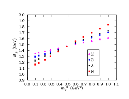
Figure 2: Masses of the octet baryons. The SU(3) flavour limit is evident. Points on the y-axis indicate the experimentally measured masses for reference.

The masses of the baryon octet are plotted against $m_{\pi}^{2}$ in Fig. 2 and are tabulated in Table 1. We observe the $SU(3)_{f}$ limit at our sixth quark mass. The mass splitting between $\Sigma$ and $\Lambda$ at the lowest pion mass ($m_{\pi}=0.3064\pm 0.0072\>\mathrm{GeV}$) on our lattice is $69\pm 2\ \mathrm{MeV}$ which is only slightly smaller than the experimentally measured splitting of $76\ \mathrm{MeV}$. Hence the generic features of the baryon-octet mass spectrum is reproduced well in our quenched simulation.

IV.2 Form factor correlators

In general, the baryon form factors are calculated on a quark-sector by quark-sector basis with each sector normalised to the contribution of a single quark with unit charge. Hence to calculate the corresponding baryon property, each quark sector contribution should be multiplied by the appropriate charge and quark number. Under such a scheme for a generic form factor $f$, the proton form factor, $f_{p}$, is obtained from the $u$- and $d$-quark sectors normalised for a single quark of unit charge via

$${f_{p}}=2\times\frac{2}{3}\times{f_{u}}+1\times\left(-\frac{1}{3}\right)\times{f_{d}}\,.$$ (44)

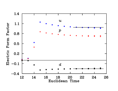
Figure 3: Electric form factor of the proton and its quark sectors (including charge and quark number factors) at $Q^{2}=0.227(2)$ $\mathrm{GeV}^{2}$ as a function of Euclidean time ($t_{2}$) for ${m}_{\pi}^{2}=0.4854\ \mathrm{GeV}^{2}$, the $SU(3)$-flavour limit. The lines indicate the fitting windows and the best fit value.

The electric form factor of the proton and contributions from the $u$- and $d$-quark sectors are plotted in Fig. 3 as a function of Euclidean time at the $SU(3)$-flavour limit. Here, charge and quark number factors have been included such that the proton result is simply the sum of the illustrated quark sectors. The lines indicate the time slices selected for the fit using the considerations of Sec. III.4.

We find that substantial Euclidean time evolution is required following the current insertion to obtain acceptable values of the $\chi^{2}/dof$; in this case seven time slices following the current insertion at $t_{1}=14$.

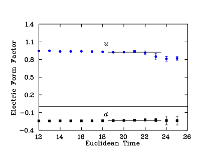
Figure 4: Quark sector contributions (including charge and quark number factors) to the electric form factor of the proton at $Q^{2}=0.227(2)$ $(\mathrm{GeV}^{2})$ as a function of Euclidean time, $t_{2}$, for the ninth quark mass where $m_{\pi}^{2}=0.2153(35)\ {\rm GeV}^{2}$. The correlator is obtained from the splitting between the ninth and eighth quark mass states. The lines indicate the fitting windows and the best fit value.

For light quark masses lighter than the strange quark mass, we fit the change in the form factor ratios of Eq. (12) from one quark mass to the next and add this to the previous result at the heavier quark mass. Figure 4 shows the quark sector contributions (including charge and quark number factors) to the electric form factor of the proton at $Q^{2}=0.227(2)$ $(\mathrm{GeV}^{2})$ as a function of Euclidean time, $t_{2}$, for the ninth quark mass where $m_{\pi}^{2}=0.2153(35)\ {\rm GeV}^{2}$. The correlator is obtained from the splitting between the ninth and eighth quark mass states. The improvement of the plateau is apparent in Fig. 4. Still substantial Euclidean time evolution is required to obtain an acceptable $\chi^{2}/dof$. The onset of noise at this lighter quark mass is particularly apparent at time slice 24 for the $d$ sector. Tables 2 to 5 list the electric form factors for all the octet baryons at the quark level for the eleven quark masses considered. In the tables, the selected time frame, the fit value and the associated $\chi^{2}/dof$ are indicated.

Table 2: Quark sector contributions to the electric form factors of the nucleon at $Q^{2}=0.227(2)\ {\rm GeV}^{2}$. Sector contributions are for a single quark having unit charge. The fit windows are selected using the criteria outlined in Sec. III.4.

$m_{\pi}^{2}$	$u_{p}$			$d_{p}$
$({\rm GeV}^{2})$	fit value	fit window	$\chi^{2}/{dof}$	fit value	fit window	$\chi^{2}/{dof}$
$0.9972(55)$	$0.798(5)$	$21-25$	$1.02$	$0.805(4)$	$21-25$	$2.36$
$0.8947(54)$	$0.789(5)$	$21-25$	$0.89$	$0.796(5)$	$21-25$	$2.53$
$0.7931(53)$	$0.779(6)$	$21-25$	$0.64$	$0.788(5)$	$21-25$	$2.21$
$0.6910(35)$	$0.768(6)$	$21-25$	$0.86$	$0.780(5)$	$21-25$	$1.57$
$0.5925(33)$	$0.756(7)$	$21-25$	$0.80$	$0.769(6)$	$21-25$	$1.42$
$0.4854(31)$	$0.740(9)$	$21-25$	$0.62$	$0.755(9)$	$21-25$	$1.19$
$0.3795(31)$	$0.725(10)$	$19-23$	$1.23$	$0.741(11)$	$19-23$	$0.78$
$0.2839(33)$	$0.708(12)$	$19-23$	$1.37$	$0.723(14)$	$19-23$	$1.31$
$0.2153(35)$	$0.693(15)$	$19-23$	$0.82$	$0.700(20)$	$19-23$	$1.23$
$0.1384(43)$	$0.682(17)$	$16-20$	$1.02$	$0.678(25)$	$16-20$	$0.89$
$0.0939(44)$	$0.666(25)$	$16-19$	$1.47$	$0.644(38)$	$16-19$	$1.28$

Table 3: Quark sector contributions to the electric form factors of $\Sigma$ baryons at $Q^{2}=0.227(2)\ {\rm GeV}^{2}$. Sector contributions are for a single quark having unit charge. The fit windows are selected using the criteria outlined in Sec. III.4.

$m_{\pi}^{2}$	$u_{\Sigma}$ or $d_{\Sigma}$			$s_{\Sigma}$
$({\rm GeV}^{2})$	fit value	fit window	$\chi^{2}/{dof}$	fit value	fit window	$\chi^{2}/{dof}$
$0.9972(55)$	$0.793(6)$	$21-25$	$0.91$	$0.759(6)$	$21-25$	$1.70$
$0.8947(54)$	$0.785(7)$	$21-25$	$0.86$	$0.758(7)$	$21-25$	$1.71$
$0.7931(53)$	$0.776(7)$	$21-25$	$0.66$	$0.757(8)$	$21-25$	$1.59$
$0.6910(35)$	$0.766(6)$	$21-25$	$1.00$	$0.757(6)$	$21-25$	$1.40$
$0.5925(33)$	$0.755(7)$	$21-25$	$0.90$	$0.756(7)$	$21-25$	$1.36$
$0.4854(31)$	$0.740(9)$	$21-25$	$0.62$	$0.755(9)$	$21-25$	$1.19$
$0.3795(31)$	$0.726(10)$	$19-23$	$1.46$	$0.754(10)$	$19-23$	$0.37$
$0.2839(33)$	$0.711(12)$	$19-23$	$1.78$	$0.753(11)$	$19-23$	$0.58$
$0.2153(35)$	$0.700(14)$	$19-23$	$0.73$	$0.752(13)$	$19-23$	$0.39$
$0.1384(43)$	$0.680(18)$	$19-21$	$0.73$	$0.754(17)$	$19-21$	$0.18$
$0.0939(44)$	$0.670(23)$	$19-23$	$1.30$	$0.750(26)$	$19-21$	$1.40$

Table 4: Quark sector contributions to the electric form factors of $\Lambda$ at $Q^{2}=0.227(2)\ {\rm GeV}^{2}$. Sector contributions are for a single quark having unit charge. The fit windows are selected using the criteria outlined in Sec. III.4.

$m_{\pi}^{2}$	$u_{\Lambda}$ or $d_{\Lambda}$			$s_{\Lambda}$
$({\rm GeV}^{2})$	fit value	fit window	$\chi^{2}/{dof}$	fit value	fit window	$\chi^{2}/{dof}$
$0.9972(55)$	$0.803(5)$	$21-25$	$1.20$	$0.745(8)$	$21-25$	$0.64$
$0.8947(54)$	$0.794(6)$	$21-25$	$1.23$	$0.744(9)$	$21-25$	$0.58$
$0.7931(53)$	$0.785(7)$	$21-25$	$1.06$	$0.744(10)$	$21-25$	$0.54$
$0.6910(35)$	$0.775(6)$	$21-25$	$1.17$	$0.738(8)$	$21-25$	$0.55$
$0.5925(33)$	$0.765(7)$	$21-25$	$1.12$	$0.737(9)$	$21-25$	$0.48$
$0.4854(31)$	$0.750(8)$	$21-25$	$1.02$	$0.735(10)$	$21-25$	$0.49$
$0.3795(31)$	$0.736(9)$	$19-23$	$0.94$	$0.734(11)$	$19-23$	$0.88$
$0.2839(33)$	$0.720(11)$	$19-23$	$1.17$	$0.730(12)$	$19-23$	$1.05$
$0.2153(35)$	$0.704(13)$	$19-23$	$1.23$	$0.727(13)$	$19-23$	$0.55$
$0.1384(43)$	$0.694(13)$	$16-19$	$3.79$	$0.727(13)$	$16-17$	$0.62$
$0.0939(44)$	$0.686(13)$	$16-17$	$2.43$	$0.729(14)$	$16-17$	$0.29$

Table 5: Quark sector contributions to the electric form factors of $\Xi$ baryons at $Q^{2}=0.227(2)\ {\rm GeV}^{2}$. Sector contributions are for a single quark having unit charge. The fit windows are selected using the criteria outlined in Sec. III.4.

$m_{\pi}^{2}$	$s_{\Xi}$			$u_{\Xi}$ or $d_{\Xi}$
$({\rm GeV}^{2})$	fit value	fit window	$\chi^{2}/{dof}$	fit value	fit window	$\chi^{2}/{dof}$
$0.9972(55)$	$0.747(9)$	$21-25$	$0.34$	$0.804(8)$	$21-25$	$1.60$
$0.8947(54)$	$0.747(9)$	$21-25$	$0.36$	$0.794(8)$	$21-25$	$1.53$
$0.7931(53)$	$0.746(10)$	$21-25$	$0.37$	$0.785(9)$	$21-25$	$1.52$
$0.6910(35)$	$0.742(8)$	$21-25$	$0.54$	$0.778(7)$	$21-25$	$1.38$
$0.5925(33)$	$0.741(8)$	$21-25$	$0.55$	$0.768(8)$	$21-25$	$1.24$
$0.4854(31)$	$0.740(9)$	$21-25$	$0.62$	$0.755(9)$	$21-25$	$1.19$
$0.3795(31)$	$0.739(9)$	$19-23$	$0.70$	$0.740(10)$	$21-25$	$1.45$
$0.2839(33)$	$0.738(10)$	$19-23$	$1.18$	$0.723(13)$	$21-25$	$1.22$
$0.2153(35)$	$0.736(10)$	$19-23$	$1.42$	$0.709(16)$	$21-25$	$0.81$
$0.1384(43)$	$0.733(10)$	$19-23$	$0.52$	$0.690(19)$	$20-23$	$0.71$
$0.0939(44)$	$0.725(11)$	$19-23$	$1.21$	$0.672(22)$	$20-23$	$0.59$

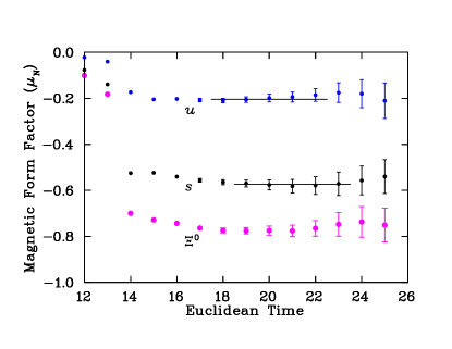
Figure 5: Magnetic form factors of $\Xi^{0}$ and its quark sectors (including charge and quark number factors) at $Q^{2}=0.227(2)$ $\mathrm{GeV}^{2}$ as a function of Euclidean time ($t_{2}$) for ${m}_{\pi}^{2}=0.4854\ \mathrm{GeV}^{2}$, the $SU(3)$-flavour limit. The lines indicate the fitting windows and the best fit value.

Turning now to the magnetic form factors, Fig. 5 shows the magnetic form factor of $\Xi^{0}$ and its quark sectors (including charge and quark number factors) as a function of Euclidean time at the $SU(3)$-flavour limit. Preferred fit windows following from the criteria of Sec. III.4 and best fit values are indicated.

Here the conversion from the natural magneton, $e/(2\,m_{B})$, where the mass of the baryon under investigation appears, to the nuclear magneton, $e/(2\,m_{N})$, where the physical nucleon mass appears, has been done by multiplying the lattice form factor results by the ratio $m_{N}/m_{B}$. In this way the form factors are presented in terms of a constant unit; i.e. the nuclear magneton.

The negative contribution of the ${u}$ quark to the total form factor indicates that its spin is on average opposite to that of the doubly represented ${s}$ quarks. This, as well the relative magnitude of the contributions, is in qualitative agreement with simple constituent quark models based on $SU(6)$ spin-flavour symmetry.

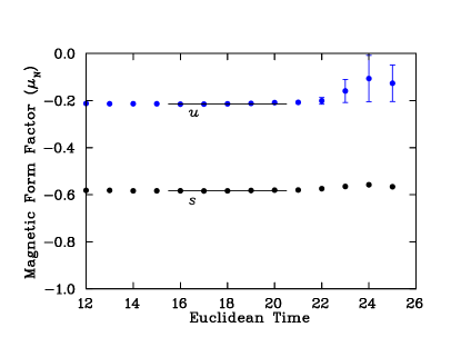
Figure 6: Quark sector contributions (including charge and quark number factors) to the magnetic form factor of $\Xi^{0}$ at $Q^{2}=0.227(2)$ $(\mathrm{GeV}^{2})$ as a function of Euclidean time, $t_{2}$, for the ninth quark mass where $m_{\pi}^{2}=0.2153(35)\ {\rm GeV}^{2}$. The correlator is obtained from the splitting between the ninth and eighth quark mass states. The lines indicate the fitting windows and the best fit value.

In Fig. 6 we present the Euclidean time dependence of the the magnetic form factors of $\Xi^{0}$ calculated at the ninth quark mass where $m_{\pi}^{2}=0.2153(35)\ {\rm GeV}^{2}$. Again the early onset of acceptable plateau behaviour is apparent here.

Results for the quark-sector contributions to the magnetic form factors of octet baryons are summarised in Tables 6 to 9.

Table 6: Quark sector contributions to the magnetic form factors of the nucleon at $Q^{2}=0.227(2)\ {\rm GeV}^{2}$. Sector contributions are for a single quark having unit charge. The fit windows are selected using the criteria outlined in Sec. III.4.

$m_{\pi}^{2}\ ({\rm GeV}^{2})$	$u_{p}\ (\mu_{N})$			$d_{p}\ (\mu_{N})$
	fit value	fit window	$\chi^{2}/{dof}$	fit value	fit window	$\chi^{2}/{dof}$
$0.9972(55)$	$0.765(12)$	$19-23$	$1.78$	$-0.295(7)$	$18-22$	$0.61$
$0.8947(54)$	$0.785(14)$	$19-23$	$1.33$	$-0.298(8)$	$18-22$	$0.51$
$0.7931(53)$	$0.804(16)$	$19-23$	$1.01$	$-0.301(9)$	$18-22$	$0.43$
$0.6931(51)$	$0.817(13)$	$19-23$	$1.00$	$-0.301(8)$	$18-22$	$0.91$
$0.5944(51)$	$0.838(15)$	$19-23$	$0.73$	$-0.304(10)$	$18-22$	$0.79$
$0.4869(50)$	$0.861(20)$	$19-23$	$0.64$	$-0.306(12)$	$18-22$	$0.86$
$0.3795(31)$	$0.893(24)$	$17-21$	$0.14$	$-0.314(14)$	$16-18$	$1.64$
$0.2839(33)$	$0.932(31)$	$17-21$	$0.14$	$-0.313(19)$	$16-19$	$1.24$
$0.2153(35)$	$0.967(42)$	$17-21$	$0.61$	$-0.313(31)$	$16-20$	$0.53$
$0.1384(43)$	$1.034(52)$	$16-20$	$1.12$	$-0.309(40)$	$15-19$	$0.49$
$0.0939(44)$	$1.024(72)$	$15-17$	$0.82$	$-0.335(54)$	$15-17$	$2.44$

Table 7: Quark sector contributions to the magnetic form factors of $\Sigma$ baryons at $Q^{2}=0.227(2)\ {\rm GeV}^{2}$. Sector contributions are for a single quark having unit charge. The fit windows are selected using the criteria outlined in Sec. III.4.

$m_{\pi}^{2}\ ({\rm GeV}^{2})$	$u_{\Sigma}\ {\rm or}\ d_{\Sigma}\ (\mu_{N})$			$s_{\Sigma}\ (\mu_{N})$
	fit value	fit window	$\chi^{2}/{dof}$	fit value	fit window	$\chi^{2}/{dof}$
$0.9972(55)$	$0.775(14)$	$19-23$	$1.22$	$-0.316(10)$	$18-22$	$0.73$
$0.8947(54)$	$0.793(16)$	$19-23$	$1.10$	$-0.314(11)$	$18-22$	$0.63$
$0.7931(53)$	$0.810(18)$	$19-23$	$0.96$	$-0.312(11)$	$18-22$	$0.55$
$0.6910(35)$	$0.821(14)$	$19-23$	$0.98$	$-0.309(9)$	$18-22$	$0.94$
$0.5925(33)$	$0.840(16)$	$19-23$	$0.82$	$-0.308(10)$	$18-22$	$0.86$
$0.4854(31)$	$0.861(20)$	$19-23$	$0.64$	$-0.306(12)$	$18-22$	$0.86$
$0.3795(31)$	$0.886(23)$	$17-21$	$0.19$	$-0.308(13)$	$16-18$	$0.42$
$0.2839(33)$	$0.914(27)$	$17-21$	$0.26$	$-0.310(15)$	$16-18$	$0.03$
$0.2153(35)$	$0.941(32)$	$17-21$	$0.61$	$-0.317(19)$	$16-18$	$0.04$
$0.1384(43)$	$0.964(33)$	$15-20$	$1.57$	$-0.317(24)$	$16-18$	$0.92$
$0.0939(44)$	$0.969(41)$	$15-17$	$0.11$	$-0.322(28)$	$16-18$	$1.08$

Table 8: Quark sector contributions to the magnetic form factors of $\Lambda$ at $Q^{2}=0.227(2)\ {\rm GeV}^{2}$. Sector contributions are for a single quark having unit charge. The fit windows are selected using the criteria outlined in Sec. III.4.

$m_{\pi}^{2}\ ({\rm GeV}^{2})$	$u_{\Lambda}\ {\rm or}\ d_{\Lambda}\ (\mu_{N})$			$s_{\Lambda}\ (\mu_{N})$
	fit value	fit window	$\chi^{2}/{dof}$	fit value	fit window	$\chi^{2}/{dof}$
$0.9972(55)$	$0.069(9)$	$19-23$	$1.26$	$1.200(22)$	$18-22$	$1.38$
$0.8947(54)$	$0.072(9)$	$19-23$	$1.20$	$1.210(22)$	$18-22$	$1.17$
$0.7931(53)$	$0.075(10)$	$19-23$	$1.07$	$1.214(24)$	$18-22$	$0.99$
$0.6910(35)$	$0.079(8)$	$19-23$	$1.08$	$1.217(17)$	$18-22$	$0.95$
$0.5925(33)$	$0.083(9)$	$19-23$	$1.00$	$1.228(18)$	$18-22$	$0.80$
$0.4854(31)$	$0.087(11)$	$19-23$	$0.88$	$1.241(21)$	$18-22$	$0.75$
$0.3795(31)$	$0.091(12)$	$17-21$	$0.55$	$1.259(22)$	$16-20$	$0.59$
$0.2839(33)$	$0.097(13)$	$17-21$	$0.29$	$1.277(25)$	$16-20$	$0.42$
$0.2153(35)$	$0.099(17)$	$17-21$	$0.36$	$1.293(28)$	$16-20$	$0.42$
$0.1384(43)$	$0.105(18)$	$15-16$	$1.79$	$1.308(33)$	$16-18$	$0.94$
$0.0939(44)$	$0.105(22)$	$15-16$	$0.19$	$1.315(37)$	$15-16$	$1.98$

Table 9: Quark sector contributions to the magnetic form factors of $\Xi$ baryons at $Q^{2}=0.227(2)\ {\rm GeV}^{2}$. Sector contributions are for a single quark having unit charge. The fit windows are selected using the criteria outlined in Sec. III.4.

$m_{\pi}^{2}\ ({\rm GeV}^{2})$	$s_{\Xi}\ (\mu_{N})$			$u_{\Xi}\ {\rm or}\ d_{\Xi}\ (\mu_{N})$
	fit value	fit window	$\chi^{2}/{dof}$	fit value	fit window	$\chi^{2}/{dof}$
$0.9972(55)$	$0.846(27)$	$19-23$	$0.60$	$-0.290(10)$	$18-22$	$0.19$
$0.8947(54)$	$0.849(27)$	$19-23$	$0.67$	$-0.294(11)$	$18-22$	$0.21$
$0.7931(53)$	$0.851(28)$	$19-23$	$0.75$	$-0.299(12)$	$18-22$	$0.21$
$0.6931(51)$	$0.855(19)$	$19-23$	$0.41$	$-0.300(10)$	$18-22$	$0.59$
$0.5944(51)$	$0.858(19)$	$19-23$	$0.49$	$-0.303(11)$	$18-22$	$0.68$
$0.4869(50)$	$0.861(20)$	$19-23$	$0.64$	$-0.306(12)$	$18-22$	$0.86$
$0.3795(31)$	$0.866(21)$	$16-20$	$0.84$	$-0.311(13)$	$16-20$	$1.77$
$0.2839(33)$	$0.871(21)$	$16-20$	$0.78$	$-0.316(14)$	$16-20$	$1.66$
$0.2153(35)$	$0.875(22)$	$16-20$	$1.04$	$-0.322(15)$	$16-20$	$0.77$
$0.1384(43)$	$0.879(22)$	$16-20$	$1.16$	$-0.328(17)$	$15-19$	$0.86$
$0.0939(44)$	$0.879(23)$	$16-20$	$0.55$	$-0.333(18)$	$15-19$	$1.00$

V DISCUSSION OF RESULTS

V.1 Charge radii

To make contact with the extensive phenomenology of the field, our results for the electric form factors are expressed in terms of charge radii. It is well known that the experimentally measured electric (and magnetic) form factor of the proton is described well by a dipole ansatz at small $Q^{2}$

$$\quad{\cal G}_{E}(Q^{2})={{\cal G}_{E}(0)\over\left(1+Q^{2}/m^{2}\right)^{2}}\,;\quad Q^{2}\geq 0\,,$$ (45)

where $m$ characterises the size of the proton. This behaviour has also been observed in recent lattice calculations Gockeler:2003ay where many momentum transfers have been considered. Using this observation, together with

$$\left\langle r_{E}^{2}\right\rangle=-6\,\frac{d}{dQ^{2}}\,{\cal G}_{E}(Q^{2})\biggm{|}_{Q^{2}=0}\ ,$$ (46)

we arrive at an expression which allows us to calculate the electric charge radius of a baryon using our two available values of the Sach’s electric form factor (${\cal G}_{E}(Q^{2}_{\rm min}),\ {\cal G}_{E}(0)$), namely

$$\frac{\left\langle r_{E}^{2}\right\rangle}{{\cal G}_{E}(0)}=\frac{12}{Q^{2}}\left(\sqrt{\frac{{\cal G}_{E}(0)}{{\cal G}_{E}(Q^{2})}}-1\right)\ .$$ (47)

While Eq. (45) is suitable for a charged baryon, alternative forms must be considered for neutral baryons where ${\cal G}_{E}(0)=0$.

However, we have direct access to the charge distributions of the individual quark sectors, a subject receiving tremendous experimental attention in the search for the role of hidden flavour in baryon structure. In this case Eq. (47) may be applied to each quark sector providing an opportunity to determine the charge radii on a sector by sector basis.

For neutral baryons it becomes a simple matter to construct the charge radii by first calculating the charge radii for each quark sector. These quark sectors are then combined using the appropriate charge and quark number factors as described in Sec. IV.2 to obtain the total baryon charge radii. Indeed, all baryon charge radii, including the charged states, are calculated in this manner.

Tables 11 to 13 provide the electric charge radii of the octet baryons and their quark-sector contributions normalised to the case of single quarks with unit charge.

Table 10: Nucleon electric charge radii squared. Quark-sector contributions are indicated for single quarks having unit charge. Baryon charge states are also summarised. Values for $m_{\pi}^{2}$ and $\langle r^{2}\rangle$ are in units of ${\rm GeV}^{2}$ and ${\rm fm}^{2}$ respectively.

$m_{\pi}^{2}$	$u_{p}$	$d_{p}$	$p$	$n$
$0.9972(55)$	$0.243(7)$	$0.231(6)$	$0.247(8)$	$-0.007(3)$
$0.8947(54)$	$0.256(8)$	$0.245(7)$	$0.259(9)$	$-0.007(3)$
$0.7931(53)$	$0.270(9)$	$0.257(8)$	$0.273(10)$	$-0.008(4)$
$0.6910(35)$	$0.288(9)$	$0.270(8)$	$0.294(10)$	$-0.012(4)$
$0.5925(33)$	$0.307(11)$	$0.286(10)$	$0.314(12)$	$-0.014(5)$
$0.4854(31)$	$0.332(14)$	$0.309(14)$	$0.340(16)$	$-0.015(7)$
$0.3795(31)$	$0.358(17)$	$0.332(17)$	$0.367(19)$	$-0.017(9)$
$0.2839(33)$	$0.389(22)$	$0.363(24)$	$0.397(24)$	$-0.017(12)$
$0.2153(35)$	$0.416(27)$	$0.403(36)$	$0.420(29)$	$-0.008(16)$
$0.1384(43)$	$0.437(31)$	$0.445(46)$	$0.435(32)$	$0.005(21)$
$0.0939(44)$	$0.467(48)$	$0.510(77)$	$0.452(53)$	$0.029(41)$

Table 11: $\Sigma$ electric charge radii squared. Quark-sector contributions are indicated for single quarks having unit charge. Baryon charge states are also summarised where absolute values of the $\Sigma^{-}$ results are reported. Values for $m_{\pi}^{2}$ and $\langle r^{2}\rangle$ are in units of ${\rm GeV}^{2}$ and ${\rm fm}^{2}$ respectively.

$m_{\pi}^{2}$	$u_{\Sigma}$ or $d_{\Sigma}$	$s_{\Sigma}$	$\Sigma^{+}$	$\Sigma^{0}$	$\Sigma^{-}$
$0.9972(55)$	$0.249(9)$	$0.301(10)$	$0.232(10)$	$-0.017(3)$	$0.266(9)$
$0.8947(54)$	$0.261(10)$	$0.302(11)$	$0.249(12)$	$-0.013(3)$	$0.275(9)$
$0.7931(53)$	$0.276(11)$	$0.304(12)$	$0.266(15)$	$-0.010(3)$	$0.285(11)$
$0.6910(35)$	$0.291(10)$	$0.304(10)$	$0.286(11)$	$-0.005(2)$	$0.295(9)$
$0.5925(33)$	$0.309(11)$	$0.306(11)$	$0.310(13)$	$0.001(3)$	$0.308(11)$
$0.4854(31)$	$0.332(14)$	$0.309(14)$	$0.340(16)$	$0.008(4)$	$0.324(13)$
$0.3795(31)$	$0.356(16)$	$0.310(15)$	$0.371(19)$	$0.015(4)$	$0.341(15)$
$0.2839(33)$	$0.382(20)$	$0.312(18)$	$0.405(23)$	$0.023(5)$	$0.359(18)$
$0.2153(35)$	$0.401(25)$	$0.315(21)$	$0.430(29)$	$0.029(6)$	$0.372(22)$
$0.1384(43)$	$0.438(33)$	$0.311(26)$	$0.480(38)$	$0.042(8)$	$0.395(28)$
$0.0939(44)$	$0.456(43)$	$0.318(41)$	$0.503(54)$	$0.046(15)$	$0.410(37)$

Table 12: $\Lambda$ electric charge radii squared. Quark-sector contributions are indicated for single quarks having unit charge. The baryon charge state is also provided. Values for $m_{\pi}^{2}$ and $\langle r^{2}\rangle$ are in units of ${\rm GeV}^{2}$ and ${\rm fm}^{2}$ respectively.

$m_{\pi}^{2}$	$u_{\Lambda}$ or $d_{\Lambda}$	$s_{\Lambda}$	$\Lambda^{0}$
$0.9972(55)$	$0.235(8)$	$0.322(13)$	$-0.029(3)$
$0.8947(54)$	$0.248(9)$	$0.323(14)$	$-0.025(3)$
$0.7931(53)$	$0.262(10)$	$0.324(15)$	$-0.021(3)$
$0.6910(35)$	$0.276(9)$	$0.335(13)$	$-0.020(3)$
$0.5925(33)$	$0.293(10)$	$0.336(14)$	$-0.014(3)$
$0.4854(31)$	$0.316(13)$	$0.340(16)$	$-0.008(4)$
$0.3795(31)$	$0.340(15)$	$0.343(18)$	$-0.001(4)$
$0.2839(33)$	$0.367(18)$	$0.350(19)$	$0.006(5)$
$0.2153(35)$	$0.395(23)$	$0.357(22)$	$0.013(6)$
$0.1384(43)$	$0.414(24)$	$0.356(22)$	$0.019(6)$
$0.0939(44)$	$0.428(25)$	$0.354(23)$	$0.025(7)$

Table 13: $\Xi$ electric charge radii squared. Quark-sector contributions are indicated for single quarks having unit charge. Baryon charge states are also summarised where absolute values of the $\Xi^{-}$ results are reported. Values for $m_{\pi}^{2}$ and $\langle r^{2}\rangle$ are in units of ${\rm GeV}^{2}$ and ${\rm fm}^{2}$ respectively.

$m_{\pi}^{2}$	$s_{\Xi}$	$u_{\Xi}$ or $d_{\Xi}$	$\Xi^{-}$	$\Xi^{0}$
$0.9972(55)$	$0.319(14)$	$0.235(11)$	$0.290(12)$	$-0.056(7)$
$0.8947(54)$	$0.320(15)$	$0.249(12)$	$0.296(13)$	$-0.047(7)$
$0.7931(53)$	$0.322(16)$	$0.262(13)$	$0.301(14)$	$-0.039(8)$
$0.6910(35)$	$0.329(13)$	$0.273(11)$	$0.310(11)$	$-0.037(6)$
$0.5925(33)$	$0.330(14)$	$0.288(12)$	$0.316(12)$	$-0.028(7)$
$0.4854(31)$	$0.332(14)$	$0.309(14)$	$0.324(13)$	$-0.015(7)$
$0.3795(31)$	$0.334(15)$	$0.333(17)$	$0.334(14)$	$-0.0003(80)$
$0.2839(33)$	$0.337(15)$	$0.361(21)$	$0.345(16)$	$0.016(10)$
$0.2153(35)$	$0.340(16)$	$0.385(27)$	$0.355(18)$	$0.029(13)$
$0.1384(43)$	$0.345(16)$	$0.419(34)$	$0.370(19)$	$0.049(19)$
$0.0939(44)$	$0.358(18)$	$0.451(41)$	$0.389(23)$	$0.062(22)$

V.1.1 Quenched chiral perturbation theory

The effective field theory formalism of quenched chiral perturbation theory (Q$\chi$PT) predicts significant contributions to the charge radii which have their origin in virtual meson-baryon loop transitions. These loops give rise to contributions which have a non-analytic dependence on the quark mass or squared pion mass. While the absence of sea-quark loops generally acts to suppress the magnitude of the coefficients of these terms (and occasionally the sign is reversed), there are several channels in which these contributions remain significant.

The leading non-analytic (LNA) and next-to-leading non-analytic (NLNA) behaviour of charge distribution radii in full QCD are

$$\langle r_{E}^{2}\rangle \!\!=\!\! \frac{1}{16\,\pi^{2}\,f^{2}}\sum_{i}\,\biggl{[}5\,\beta_{i}\,\log\left(\frac{m_{i}^{2}}{\mu^{2}}\right)-10\,\beta^{\prime}_{i}\,{\cal G}(m_{i},\Delta,\mu)$$ (48)

$$+c_{0}+c_{2}\,m_{i}^{2}+c_{4}\,m_{i}^{4}\ldots\biggr{]}\ .$$

Here the sum over $i$ includes the $\pi$ and $K$ pseudoscalar mesons. The contributions of the various charge states of these mesons are contained in the coefficients $\beta$ and $\beta^{\prime}$, reflecting electric charge and SU(3) axial couplings, $D$, $F$ and $C$. In quenching the theory, the coefficients $\beta$ and $\beta^{\prime}$ are modified to reflect the absence of sea-quark loops.

The first term arises from octet baryon to octet-baryon – meson transitions. Thus charge radii are characterised by a logarithmic divergence Leinweber:1992hj in the chiral limit ($m_{\pi}^{2}\rightarrow 0$). In this simple form, the mass splittings between baryon octet members is neglected.

The second term of Eq. (48) arises from octet baryon to decuplet-baryon – meson transitions. As the splitting between the baryon octet and decuplet does not vanish in the chiral limit, the mass splitting, $\Delta=M_{\Delta}-M_{N}$, between the nucleon and $\Delta$ for example, plays an important role. The function ${\cal G}(m_{i},\Delta,\mu)$ is

$${\cal G}(m,\Delta,\mu)=\log\left(\frac{m^{2}_{i}}{\mu^{2}}\right)-$$ (49)

$$\frac{\Delta}{\sqrt{\Delta^{2}-m_{i}^{2}}}\log\frac{\Delta-\sqrt{\Delta^{2}-m_{i}^{2}+i\epsilon}}{\Delta+\sqrt{\Delta^{2}-m_{i}^{2}+i\epsilon}}\ .$$

As the tadpole graph contributing to the LNA term of charge radii in full QCD vanishes in quenched QCD Arndt:2004 , the coefficients $\beta$ and $\beta^{\prime}$ for charge radii are identical to those for magnetic moments in quenched QCD Leinweber:2002qb ; Savage:2001dy . Figure 7 displays the non-analytic contributions from Q$\chi$PT as given in Eq. (48), plotted for the sample case of the proton. In this case, the values of $\beta$ and $\beta^{\prime}$ are $-\frac{4}{3}D^{2}$ and $-\frac{1}{6}C^{2}$ respectively Leinweber:2002qb ; Savage:2001dy . Here the axial couplings $D$ and $C$ are related by $C=2D$ and $D$ is taken as $0.76$. The scale $\mu^{2}$ is taken to be 1 GeV² and serves only to define $c_{0}$.

Because these non-analytic contributions are complemented by terms analytic in the quark mass or pion-mass squared, the slope and curvature at large $m_{\pi}^{2}$ of these contributions is not significant. What is significant is the curvature at small $m_{\pi}^{2}$ and we see that this curvature is dominated by the LNA term. Here there is no mass splitting to mask the effects of dynamical chiral symmetry breaking. Thus, we will examine the extent to which our simulation results are consistent with the LNA behaviour of Q$\chi$PT.

The coefficient $\beta$ is related to the coefficient of the leading non-analytic (LNA) contribution to the magnetic moment, $\chi$, via the relation Leinweber:2002qb

$$\beta\frac{m_{N}}{8\pi f_{\pi}^{2}}=\chi\ .$$ (50)

The coefficients $\chi$ have been determined for octet baryons and their individual quark sector contributions in Ref. Leinweber:2002qb and numerical values are reproduced in Tables 14 and 15 for ready reference.

Since $m_{\pi}^{2}<1\ {\rm GeV}^{2}$ in our simulations, the logarithmic term is negative for all quark masses considered here. Hence, the charge radius will exhibit a logarithmic divergence in chiral limit to either positive or negative infinity, depending on the whether $\beta$ (or $\chi$) is negative or positive respectively.

Figure 7: The leading (upper curve) and next-to-leading (lower curve) non-analytic contributions to the charge radius of the proton as given by quenched chiral perturbation theory in Eq. (48).

In the quenched approximation, the flavour-singlet $\eta^{\prime}$ meson remains degenerate with the pion and makes important contributions to quenched chiral non-analytic behaviour. The neutrality of its charge prevents it from contributing to the coefficients of Tables 14 and 15. However, the double hair-pin diagram in which the vector current couples to the virtual baryon intermediary does give rise to chirally-singular behaviour. However the relatively small couplings render these contributions small at the quark masses probed here.

Table 14: Coefficients, $\chi$, providing the LNA contribution to baryon magnetic moments and charge radii in quenched QCD. Coefficients for magnetic moments in full QCD are also indicated. Here the coefficients for quark sector contributions to baryon properties are indicated for quarks having unit charge. Note that $u_{p}$ for example denotes the coefficient for the two $u$ quarks of the proton, each of which have unit charge. Intermediate (Int.) meson-baryon channels are indicated to allow for $SU(3)$-flavour breaking in both the meson and baryon masses. The coefficients are calculated from the expressions of Ref. Leinweber:2002qb with the axial couplings $F=0.50$ and $D=0.76$ with $f_{\pi}=93$ MeV.

$q$	Int.	Full QCD	Quenched QCD
$u_{p}\mid d_{n}$	$N\pi$	$-6.87$	$-3.33$
	$\Lambda K$	$-3.68$	$0$
	$\Sigma K$	$-0.15$	$0$
$d_{p}\mid u_{n}$	$N\pi$	$+6.87$	$+3.33$
	$\Sigma K$	$-0.29$	$0$
$s_{p}\mid s_{n}$	$\Lambda K$	$+3.68$	$0$
	$\Sigma K$	$+0.44$	$0$
$u_{\Sigma^{+}}\mid d_{\Sigma^{-}}$	$\Sigma\pi$	$-2.16$	$0$
	$\Lambda\pi$	$-1.67$	$0$
	$NK$	$0$	$-0.29$
	$\Xi K$	$-6.87$	$-3.04$
$d_{\Sigma^{+}}\mid u_{\Sigma^{-}}$	$\Sigma\pi$	$+2.16$	$0$
	$\Lambda\pi$	$+1.67$	$0$
	$NK$	$+0.29$	$0$
$s_{\Sigma}$	$NK$	$-0.29$	$+0.29$
	$\Xi K$	$+6.87$	$+3.04$
	$\Sigma\eta_{s}$	$0$	$0$
$u_{\Sigma^{0}}\mid d_{\Sigma^{0}}$	$\Sigma\pi$	$0$	$0$
	$\Lambda\pi$	$0$	$0$
	$NK$	$+0.15$	$-0.15$
	$\Xi K$	$-3.43$	$-1.52$
$u_{\Lambda}\mid d_{\Lambda}$	$\Sigma\pi$	$0$	$0$
	$\Lambda\eta_{l}$	$0$	$0$
	$NK$	$+3.68$	$+1.23$
	$\Xi K$	$-0.40$	$+0.44$
$s_{\Lambda}$	$\Lambda\eta_{s}$	$0$	$0$
	$NK$	$-7.36$	$-2.45$
	$\Xi K$	$+0.79$	$-0.88$
$u_{\Xi^{0}}\mid d_{\Xi^{-}}$	$\Xi\pi$	$-0.29$	$0$
	$\Lambda K$	$0$	$-0.40$
	$\Sigma K$	$+6.87$	$+3.43$
	$\Omega K$	$0$	$+0.29$
$d_{\Xi^{0}}\mid u_{\Xi^{-}}$	$\Xi\pi$	$+0.29$	$0$
	$\Lambda K$	$+0.40$	$0$
	$\Sigma K$	$+3.43$	$0$
$s_{\Xi}$	$\Lambda K$	$-0.40$	$+0.40$
	$\Sigma K$	$-10.3$	$-3.43$
	$\Omega K$	$0$	$-0.29$
	$\Xi\eta_{s}$	$0$	$0$

Table 15: Coefficients, $\chi$, providing the LNA contribution to baryon magnetic moments and charge radii in quenched QCD. Coefficients for magnetic moments in full QCD are also indicated. Intermediate (Int.) meson-baryon channels are indicated to allow for $SU(3)$-flavour breaking in both the meson and baryon masses. The coefficients are calculated from the expressions of Ref. Leinweber:2002qb with the axial couplings $F=0.50$ and $D=0.76$ with $f_{\pi}=93$ MeV.

Baryon	Channel	Full QCD	Quenched QCD
$p$	$N\pi$	$-6.87$	$-3.33$
	$\Lambda K$	$-3.68$	$0$
	$\Sigma K$	$-0.15$	$0$
$n$	$N\pi$	$+6.87$	$+3.33$
	$\Lambda K$	$0$	$0$
	$\Sigma K$	$-0.29$	$0$
$\Sigma^{+}$	$\Sigma\pi$	$-2.16$	$0$
	$\Lambda\pi$	$-1.67$	$0$
	$NK$	$0$	$-0.29$
	$\Xi K$	$-6.87$	$-3.04$
	$\Sigma\eta_{s}$	$0$	$0$
$\Sigma^{0}$	$\Sigma\pi$	$0$	$0$
	$\Lambda\pi$	$0$	$0$
	$NK$	$+0.15$	$-0.15$
	$\Xi K$	$-3.43$	$-1.52$
	$\Sigma\eta_{s}$	$0$	$0$
$\Sigma^{-}$	$\Sigma\pi$	$+2.16$	$0$
	$\Lambda\pi$	$+1.67$	$0$
	$NK$	$+0.29$	$0$
	$\Xi K$	$0$	$0$
	$\Sigma\eta_{s}$	$0$	$0$
$\Lambda$	$\Sigma\pi$	$0$	$0$
	$\Lambda\eta_{l}$	$0$	$0$
	$NK$	$+3.68$	$+1.23$
	$\Xi K$	$-0.40$	$+0.44$
	$\Lambda\eta_{s}$	$0$	$0$
$\Xi^{0}$	$\Xi\pi$	$-0.29$	$0$
	$\Lambda K$	$0$	$-0.40$
	$\Sigma K$	$+6.87$	$+3.43$
	$\Omega K$	$0$	$+0.29$
	$\Xi\eta_{s}$	$0$	$0$
$\Xi^{-}$	$\Xi\pi$	$+0.29$	$0$
	$\Lambda K$	$+0.40$	$0$
	$\Sigma K$	$+3.43$	$0$
	$\Omega K$	$0$	$0$
	$\Xi\eta_{s}$	$0$	$0$

V.1.2 Quark sector charge radii

We begin with an examination of the quark contributions to baryon charge radii. The results are reported for single quarks of unit charge. Of particular interest are the contributions of similar quarks experiencing different environments. Traditionally, quark models of hadron structure neglected such environment sensitivity. However, such environment sensitivity is manifest in chiral effective field theory. The finite kaon mass in the chiral limit renders the kaon’s contributions to curvature almost trivial relative to the pion.

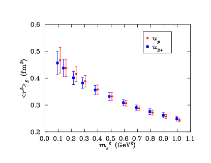
Figure 8: Electric charge radii of the $u$-quark distribution in the proton, ${u_{p}}$, and $\Sigma^{+}$, ${u}_{\Sigma^{+}}$, as a function of $m_{\pi}^{2}$ representing the quark masses considered in the simulation. The results for ${u_{p}}$ are offset for clarity.

Figure 8 displays the charge radii of the ${u}$-quark distribution in the proton and compares this with the ${u}$-quark distribution in $\Sigma^{+}$. The $SU(3)$-flavour limit is manifest at $m_{\pi}^{2}\sim 0.5$ GeV². The replacement of a $d$-quark in the proton, by an $s$ quark in $\Sigma^{+}$ gives rise to only a small environment sensitivity in the $u$-quark properties.

Referring to the chiral coefficients of Table 14, the negative value of $\chi$ for $u_{p}$ indicates that the charge radius of the $u$ quark distribution in the proton should diverge to positive infinity in the chiral limit. A physical understanding of this is made obvious by considering the virtual transition $p\to n\pi^{+}$, which at the quark level can be understood as $(uud)\to(udd)(\overline{d}u)$. In the chiral limit, the $\pi^{+}$ carries the $u$ quark to infinity such that $u$-quark charge distribution radius in the proton diverges.

In the case of the $u$ quark in $\Sigma^{+}$, the coefficient of the logarithmic divergence is zero in the $\pi$ channel and hence no divergence is expected. While there is a significant coefficient for transitions to $\Xi K$, the increased mass of the $\Xi$ baryon makes this channel unfavourably suppressed.

The results in Fig. 8 for $u_{p}$ exhibit an upward trend and increasing curvature with reducing quark mass. The $u_{\Sigma^{+}}$ rises more slowly. Hence these results are in qualitative agreement with the LNA expectations of chiral effective field theory.

Figure 9: Charge radii of ${u_{n}}$ and ${u}_{\Xi^{0}}$ as a function of $m_{\pi}^{2}$. The data for the ${u_{n}}$ are offset for clarity.

Figure 9 displays the electric charge radii of the $u$ quark in the neutron ($u_{n}$) and in $\Xi^{0}$ ($u_{\Xi^{0}}$) as a function of $m_{\pi}^{2}$. Here we observe that the charge radii of $u_{n}$ and $u_{\Xi^{0}}$ are nearly equal at heavy quark masses, but in the chiral limit they differ. The light $d$-quark environment of the ${u}$ quark in the neutron provides enhanced chiral curvature as the chiral limit is approached.

However, the true nature of the underlying physics is much more subtle. From Table 14, we see that the quenched coefficient (last column) for the ${u}$ quark in the neutron is positive in the $\pi$ channel, from which we can deduce that the charge radius should actually diverge to negative infinity in the chiral limit.

Physically this can be understood by looking at the quark contributions to the virtual transition $n\to p\pi^{-}$ which gives rise to this divergence. In this case one has $(ddu)\to(duu)(\overline{u}d)$. In the chiral limit, the mass of the pion approaches zero such that the $\pi^{-}$ carries a $\overline{u}$ quark to infinity. Since the $d$ quark is ignored while calculating the $u$ quark contribution (i.e. the electric charge of the $d$ quark may be thought of as zero), the entire charge of the pion comes from the $\overline{u}$ quark, thus taking the $u$-quark charge distribution radius to negative infinity. However, Fig. 9 shows no such trend.

The coefficient $\chi$ for $u_{\Xi^{0}}$ is zero in the $\pi$ channel, indicating that there should be no logarithmic divergence in the chiral limit. However it does have a substantial positive coefficient in the favourable $\Sigma K$ channel, indicating the possibility of downward curvature as the chiral limit is approached. Again, Fig. 9 shows no hint of downward curvature.

While the statistical error bars are sufficiently large to hide such a turn over, there are other interpretations. One possibility is that we are not yet in the true chiral regime where such physics is manifest. Indeed, the divergence of the $u$-quark charge distribution to negative infinity may only reveal itself at quark masses lighter than the physical quark masses.

Alternatively, one might regard this particular case to be somewhat exceptional. It is the only channel in which chiral-loop physics is expected to oppose the natural broadening of a distribution’s Compton wavelength. On the lattice, the finite volume restricts the low momenta of the effective field theory to discrete values. It may be that this lattice artifact prevents one from building up sufficient strength in the loop integral to counter the Compton broadening. In this case it would be impossible to observe the divergence of $u_{n}\to-\infty$ at any quark mass. It will be interesting to resolve this discrepancy with quantitative effective field theory calculations.

Figure 10: Electric charge distribution radius of a $u$ quark in $\Lambda$ as a function of $m_{\pi}^{2}$.

Figure 10 reports our results for the charge distribution radius of a $u$ quark in $\Lambda$ as a function of $m_{\pi}^{2}$. The chiral coefficient for this is zero in the $\pi$ channel and hence no divergence is expected. However, there is significant strength for downward curvature in the energetically favourable $NK$ channel. Indeed, the approach to the chiral limit is remarkably linear and contrasts the upward curvature observed for other light quark flavours. Hence our results are in qualitative agreement with the expectations of Q$\chi$PT.

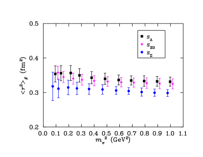
Figure 11: Electric charge distribution radii of strange quarks including ${s}_{\Lambda}$, ${s}_{\Xi^{0}}$ and ${s}_{\Sigma^{0}}$. The data for ${s}_{\Xi^{0}}$ and ${s}_{\Lambda}$ are plotted at shifted ${m}^{2}_{\pi}$ values for clarity.

Figure 11 illustrates the charge distribution radius of strange quarks in $\Lambda^{0}$, $\Xi^{0}$ and $\Sigma^{0}$. In our simulations the strange quark mass is held fixed and therefore any variation observed in the results is purely environmental in origin. All three distributions suggest a gentle dependence on the mass of the environmental light quarks.

However, the environmental flavour-symmetry dependence of the strange quark distributions is absolutely remarkable. When the environmental quarks are in an isospin 0 state in the $\Lambda$, the strange quark distribution is broad. On the other hand, when the environmental quarks are in an isospin 1 state in $\Sigma$ baryons, the distribution radius is significantly smaller.

In the case of strange quark distributions, the LNA contributions are exclusively from transitions involving the kaon. Therefore significant curvature is not expected. On the other hand, one might expect broader distributions in cases where a virtual transition is possible in quenched QCD. Referring to Table 14, one sees that both $s_{\Lambda}$ and $s_{\Xi}$ have strong transitions to the energetically favourable $KN$ and $K\Sigma$ channels respectively. The coefficients are negative such that the virtual transitions will act to enhance the charge distributions. This is not the case for $s_{\Sigma}$ where the sign is positive and the transition is to the energetically unfavoured $K\Xi$ channel. In summary, Q$\chi$PT suggests the charge distributions for $s_{\Lambda}$ and $s_{\Xi}$ will be larger than for $s_{\Sigma}$. This is exactly what is observed in Figure 11.

V.1.3 Baryon charge radii

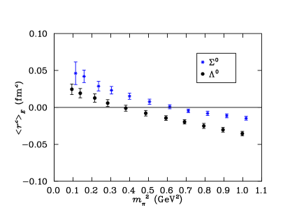
Figure 12: Electric charge radii of $\Sigma^{0}$ and $\Lambda^{0}$ as a function of $m_{\pi}^{2}$. The data for $\Sigma^{0}$ is offset to the right for clarity.

The flavour-symmetry dependence of $uds$-quark distributions in $\Sigma^{0}$ and $\Lambda^{0}$ is particularly manifest in Fig. 12. Here the interplay between the light-quark sector with effective charge $1/3$ and the strange sector with charge $-1/3$ is revealed.

At the $SU(3)$ flavour-symmetric point ($m_{\pi}^{2}\sim 0.5\ {\rm GeV}^{2}$) where the strange and light quarks have the same mass and the $\Lambda$ and $\Sigma$ are degenerate in mass, neither charge radius is zero. This very nicely reveals different charge distributions for the quark sectors described in the previous section.

In constituent quark models, this flavour dependence would be described in terms of spin-dependent forces. In the $\Lambda^{0}$ where a scalar diquark can form between the non-strange pair, the charge radius is dominated by the broader strange-quark distribution at the $SU(3)$-flavour symmetric point. This is contrasted by the $\Sigma^{0}$ where scalar-diquark pairing would occur between strange and non-strange quarks, acting to constrict the strange quark distribution in $\Sigma$ as seen in Fig. 11. In addition, hyperfine repulsion in the non-strange quark sector leads to a broader distribution for the light quark sector as indicated in Tables 11 and 13. As compelling as this discussion is, this line of reasoning suggests the decuplet baryon states should have broader quark distributions Leinweber:1993nr as scalar-diquark clusters do not dominate there. However, preliminary results from an analysis of decuplet baryon structure on the same lattice configurations explored here newDecuplet , do not reveal broader quark distributions. For this reason, we consider our discussion of virtual transitions in the context of effective field theory in the previous section to be a more relevant description of the underlying physics.

Ultimately, as the chiral limit is approached, the light quark distribution broadens and dominates the charge radii for both baryons. However, the charge distribution of the $\Sigma^{0}$ is much broader and reflects our discussion of the quark sector contributions. In particular, the LNA contributions of Q$\chi$PT act to suppress the distribution of $u_{\Lambda}$ and enhance $s_{\Lambda}$, whereas the LNA contributions to $\Sigma^{0}$ are relatively suppressed either by having small coefficients or having energetically unfavourable transitions in the kaon channel. This suppression of $u_{\Lambda}$ and enhancement $s_{\Lambda}$ combines to give a strong net effect of suppressing the charge radius of the $\Lambda^{0}$.

Figure 13: Electric charge radii of charged hyperons. The $\Xi^{-}$ and $\Sigma^{+}$ are offset to the left and right respectively for clarity.

The hyperon charge states, $\Sigma^{-}$ and $\Xi^{-}$ have chiral coefficients which vanish in quenched QCD. Similarly, $\Sigma^{+}$ has no contributions from virtual pion transitions. The one case, where there is a substantial coefficient, is suppressed energetically. Figure 13 displays our simulation results for the electric charge distribution radii of these hyperons as a function of $m_{\pi}^{2}$. The ordering of the charge radii as the chiral limit is approached is explained by the more localized strange quark distribution.

Figure 14: Electric charge radii of the proton and $\Sigma^{+}$. Charge radii for $\Sigma^{+}$ are offset for clarity.

Figure 14 compares the charge radii of $\Sigma^{+}$ with the proton. The charge radii of these baryons match at the SU(3) flavour limit where $m_{\pi}^{2}\sim 0.5\ {\rm GeV}^{2}$ as required. As the chiral limit is approached, the smaller charge distribution of the heavier negatively-charged strange quark acts to make the $\Sigma^{+}$ larger. This is manifest in the simulation results.

While the $\Sigma^{+}$ is not expected to display chiral curvature, the proton charge radius presents one of the more favourable opportunities to observe a hint of the logarithmic divergence to be encountered in the chiral and infinite-volume limits of quenched QCD. However, there is no hint of chiral curvature in favour of the proton over the $\Sigma^{+}$.

The origin of this discrepancy is once again traced to the singly-represented $u$-quark in the neutron, or more specifically in this case, the singly-represented $d$-quark in the proton. As highlighted in the discussion surrounding Fig. 8, there is a hint of increased curvature for the doubly-represented $u$-quark in the proton over that in $\Sigma$, in accord with chiral effective field theory. But this is hidden in the proton charge radius due to the absence of the anticipated curvature of the singly-represented quark in the nucleon, as highlighted in the discussion surrounding Fig. 9.

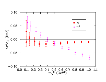
Figure 15: Electric charge radii of the neutron and $\Xi^{0}$. Charge radii for the $\Xi^{0}$ are shifted to the right for clarity. Asymmetric error bars for the neutron charge radius are described in the text.

Similarly, the ultimate divergence of the neutron charge radius to negative infinity via $n\to p\pi^{-}$ is not yet manifest. Rather a crossing of the central values into positive values of squared charge radii is revealed in Fig. 15. Still, the statistical errors remain consistent with negative values.

The crossing of the central values of the squared neutron charge radius into positive values led us to further examine our selection of fit regime in our correlation function analysis. Our concern is that noise in the correlation function may be distorting the fit. Hence, we have also considered fits including $t=15$, immediately following the point-split current insertion centred at $t=14$. While we prefer to allow some Euclidean time evolution following the current insertion, this systematic uncertainty is reflected in the asymmetric error bar of Fig. 15 for the lightest two neutron charge radii.

To summarise, we have explored the electric form factors of the baryon octet and their quark sector contributions at light quark masses approaching the chiral regime. The unprecedented nature of our quark masses is illustrated in Fig. 16 which compares the present results for the proton charge radius with the previous state of the art Leinweber:1990dv ; Wilcox:1991cq . Here the static quark potential has been used to uniformly set the scale among all the results. The small values of the early results are most likely due to the small physical lattice volumes necessitated at that time. The precision afforded by 400 $20^{3}\times 40$ lattices is manifest.

We have discovered that all baryons having non-vanishing energetically-favourable couplings to virtual meson-baryon transitions tend to be broader than those which do not. This qualitative realisation provides a simple explanation for the patterns revealed in our quenched-QCD simulations.

Still, evidence of chiral curvature on our large-volume lattice is rather subtle in general and absent in the exceptional case of the singly-represented quark in the neutron or $\Xi$. In this case, it is thought that the restriction of momenta to discrete values on the finite-volume lattice prevents the build up of strength in the loop integral of effective field theory. Without sufficient strength, the Compton broadening of the distribution will not be countered as the chiral limit is approached.

Figure 16: The proton charge radius is compared with previous state of the art lattice simulation results in quenched QCD. The solid squares indicate current lattice QCD results with FLIC fermions. The stars indicate the lattice results of Leinweber:1990dv while the crosses indicate the results of Wilcox:1991cq , both of which use the standard Wilson actions for the gauge and fermion fields.

V.2 Magnetic moments

The magnetic moment $\mu$ is provided by the magnetic form factor at $Q^{2}=0$, ${\cal{G}}_{M}(0)$, with units of the natural magneton, $\mu_{B}={e}/({2\,M_{B}})$, where $M_{B}$ is the mass of the baryon

$$\mu={\cal{G}}_{M}(0)\,\frac{e}{2M_{B}}\,.$$ (51)

While we could present a detailed discussion of the magnetic form factors summarised in Sec. IV.2, a more interesting discussion of the results is facilitated via the magnetic moment where chiral non-analytic behaviour takes on a simple functional form and a vast collection of phenomenology is available to provide a context for our results.

Since the magnetic form factors must be calculated at a finite value of momentum transfer, $Q^{2}$, the magnetic moment must be inferred from our results, ${\cal{G}}_{M}(Q^{2})$, obtained at the minimum non-vanishing momentum transfer available on our periodic lattice. The $Q^{2}$ dependence of lattice results from the QCDSF collaboration Gockeler:2003ay are described well by a dipole. Phenomenologically this is a well established fact for the nucleon at low momentum transfers.

However, we will take an even weaker approximation and assume only that the $Q^{2}$ dependence of the electric and magnetic form factors is similar, without stating an explicit functional form for the $Q^{2}$ dependence. This too is supported by experiment where the proton ratio $\frac{{\cal{G}}_{M}(Q^{2})}{\mu\,{\cal{G}}_{E}(Q^{2})}\simeq 1$ for values of $Q^{2}$ similar to that probed here. In this case

$${\cal{G}}_{M}(0)=\frac{{\cal{G}}_{M}(Q^{2})}{{\cal{G}}_{E}(Q^{2})}\,{\cal{G}}_{E}(0)\,.$$ (52)

The strange and light sectors of hyperons will scale differently, and therefore we apply Eq. (52) to the individual quark sectors. Octet baryon properties are then reconstructed as described in the discussion surrounding Eq. (44) in Sec. IV.2. Results for baryon magnetic moments and their quark sector contributions are summarised in Tables 17 through 19.

Table 16: Nucleon magnetic moments and their quark sector contributions. Sector contributions are indicated for single quarks having unit charge. Baryon charge states are also summarised. Values for $m_{\pi}^{2}$ and magnetic moments are in units of ${\rm GeV}^{2}$ and $\mu_{N}$ respectively.

$m_{\pi}^{2}$	$u_{p}$	$d_{p}$	$p$	$n$
$0.9972(55)$	$0.960(13)$	$-0.366(8)$	$1.401(18)$	$-0.883(11)$
$0.8947(54)$	$0.995(15)$	$-0.373(9)$	$1.451(21)$	$-0.913(12)$
$0.7931(53)$	$1.032(18)$	$-0.382(10)$	$1.503(25)$	$-0.943(14)$
$0.6910(35)$	$1.064(14)$	$-0.386(10)$	$1.547(19)$	$-0.967(12)$
$0.5925(33)$	$1.108(17)$	$-0.395(12)$	$1.610(24)$	$-1.002(15)$
$0.4854(31)$	$1.163(24)$	$-0.406(16)$	$1.686(33)$	$-1.046(20)$
$0.3795(31)$	$1.231(29)$	$-0.424(20)$	$1.783(41)$	$-1.104(25)$
$0.2839(33)$	$1.317(41)$	$-0.433(28)$	$1.901(57)$	$-1.167(36)$
$0.2153(35)$	$1.395(62)$	$-0.447(47)$	$2.009(87)$	$-1.228(56)$
$0.1384(43)$	$1.517(79)$	$-0.456(60)$	$2.17(11)$	$-1.315(71)$
$0.0939(44)$	$1.54(11)$	$-0.521(87)$	$2.22(15)$	$-1.372(92)$

Table 17: $\Sigma$ magnetic moments and their quark sector contributions. Sector contributions are indicated for single quarks having unit charge. Baryon charge states are also summarised. Values for $m_{\pi}^{2}$ and magnetic moments are in units of ${\rm GeV}^{2}$ and $\mu_{N}$ respectively.

$m_{\pi}^{2}$	$u_{\Sigma^{+}}$	$s_{\Sigma}$	$\Sigma^{+}$	$\Sigma^{0}$	$\Sigma^{-}$
$0.9972(55)$	$0.976(15)$	$-0.416(13)$	$1.440(21)$	$0.464(7)$	$-0.512(10)$
$0.8947(54)$	$1.010(18)$	$-0.414(14)$	$1.484(24)$	$0.474(8)$	$-0.535(12)$
$0.7931(53)$	$1.044(21)$	$-0.412(15)$	$1.530(28)$	$0.485(9)$	$-0.559(14)$
$0.6910(35)$	$1.072(15)$	$-0.408(12)$	$1.565(21)$	$0.493(7)$	$-0.579(11)$
$0.5925(33)$	$1.113(18)$	$-0.407(14)$	$1.620(26)$	$0.507(8)$	$-0.607(13)$
$0.4854(31)$	$1.163(24)$	$-0.406(16)$	$1.686(33)$	$0.523(10)$	$-0.640(16)$
$0.3795(31)$	$1.221(27)$	$-0.409(18)$	$1.764(38)$	$0.543(12)$	$-0.678(18)$
$0.2839(33)$	$1.286(34)$	$-0.412(21)$	$1.852(47)$	$0.566(14)$	$-0.720(22)$
$0.2153(35)$	$1.344(42)$	$-0.421(27)$	$1.932(58)$	$0.588(18)$	$-0.756(28)$
$0.1384(43)$	$1.418(50)$	$-0.421(34)$	$2.031(72)$	$0.613(23)$	$-0.805(32)$
$0.0939(44)$	$1.446(77)$	$-0.429(42)$	$2.07(11)$	$0.625(30)$	$-0.821(53)$

Table 18: The $\Lambda^{0}$ magnetic moment and its quark sector contributions. Sector contributions are indicated for single quarks having unit charge. Baryon charge states are also summarised. Values for $m_{\pi}^{2}$ and magnetic moments are in units of ${\rm GeV}^{2}$ and $\mu_{N}$ respectively.

$m_{\pi}^{2}$	$u_{\Lambda}$	$s_{\Lambda}$	$\Lambda^{0}$
$0.9972(55)$	$0.086(10)$	$1.611(29)$	$-0.509(9)$
$0.8947(54)$	$0.091(12)$	$1.621(20)$	$-0.510(10)$
$0.7931(53)$	$0.095(13)$	$1.631(32)$	$-0.512(10)$
$0.6910(35)$	$0.102(11)$	$1.650(21)$	$-0.516(8)$
$0.5925(33)$	$0.109(12)$	$1.666(24)$	$-0.519(8)$
$0.4854(31)$	$0.117(14)$	$1.688(28)$	$-0.524(10)$
$0.3795(31)$	$0.124(16)$	$1.715(32)$	$-0.530(11)$
$0.2839(33)$	$0.135(18)$	$1.749(37)$	$-0.538(13)$
$0.2153(35)$	$0.140(24)$	$1.780(43)$	$-0.547(16)$
$0.1384(43)$	$0.151(27)$	$1.799(49)$	$-0.549(18)$
$0.0939(44)$	$0.154(31)$	$1.804(53)$	$-0.550(20)$

Table 19: $\Xi$ magnetic moments and their quark sector contributions. Sector contributions are indicated for single quarks having unit charge. Baryon charge states are also summarised. Values for $m_{\pi}^{2}$ and magnetic moments are in units of ${\rm GeV}^{2}$ and $\mu_{N}$ respectively.

$m_{\pi}^{2}$	$s_{\Xi}$	$u_{\Xi^{0}}$	$\Xi^{0}$	$\Xi^{-}$
$0.9972(55)$	$1.132(32)$	$-0.361(13)$	$-0.996(23)$	$-0.635(22)$
$0.8947(54)$	$1.137(33)$	$-0.371(14)$	$-1.005(24)$	$-0.634(23)$
$0.7931(53)$	$1.141(34)$	$-0.381(15)$	$-1.015(24)$	$-0.634(24)$
$0.6910(35)$	$1.152(21)$	$-0.385(13)$	$-1.025(18)$	$-0.640(14)$
$0.5925(33)$	$1.157(22)$	$-0.395(14)$	$-1.035(19)$	$-0.640(15)$
$0.4854(31)$	$1.163(24)$	$-0.406(16)$	$-1.046(20)$	$-0.640(16)$
$0.3795(31)$	$1.172(24)$	$-0.421(18)$	$-1.062(21)$	$-0.641(17)$
$0.2839(33)$	$1.181(25)$	$-0.437(20)$	$-1.079(23)$	$-0.642(17)$
$0.2153(35)$	$1.189(27)$	$-0.454(23)$	$-1.096(25)$	$-0.642(18)$
$0.1384(43)$	$1.199(29)$	$-0.475(27)$	$-1.116(29)$	$-0.641(20)$
$0.0939(44)$	$1.212(29)$	$-0.495(31)$	$-1.138(32)$	$-0.643(20)$

V.2.1 Quenched chiral perturbation theory

As for the charge radii, it is interesting to compare our results with the LNA and NLNA terms of $\chi$PT which survive to some extent in Q$\chi$PT. As for the charge radii, the NLNA contributions provide little curvature Young:2004tb and we turn our attention to the LNA contributions Leinweber:2002qb . These LNA contributions to baryon magnetic moments have their origin in couplings of the electromagnetic current to the virtual meson propagating in the intermediate meson-baryon state.

For virtual pion transitions, the LNA terms have the very simple form $\chi\,m_{\pi}\sim{m_{q}}^{1/2}$, with values for $\chi$ as summarised in Tables 14 and 15. While this contribution is finite in the chiral limit, the rate of change of this contribution does indeed diverge in the chiral limit. The less singular nature of this contribution should allow its contributions to be observed at larger pion masses, making magnetic moments an excellent observable to consider in searching for evidence of chiral curvature. Kaon contributions take on the same form in the limit in which baryon mass splittings are neglected.

As for the charge radii, negative values of $\chi$ provide curvature towards more positive values as the chiral limit is approached, and vice versa for positive values of $\chi$.

As emphasised earlier in our discussion of charge radii, the flavour-singlet $\eta^{\prime}$ meson remains degenerate with the pion in the quenched approximation and makes important contributions to quenched chiral non-analytic behaviour. The neutrality of its charge prevents it from contributing to the coefficients of Tables 14 and 15. However, the double hair-pin diagram in which the vector current couples to the virtual baryon intermediary does give rise to a logarithmic divergence in baryon magnetic moments. However the relatively small couplings of the $\eta^{\prime}$ render these contributions negligible at the quark masses probed here Young:2004tb .

V.2.2 Quark sector magnetic moments

Figure 17: Magnetic moment contributions of the $u$-quark sector to the proton, ${u_{p}}$, and the $\Sigma^{+}$, ${u}_{\Sigma^{+}}$. The contributions ${u_{p}}$ are shifted right for clarity.

The $u$-quark contribution to the proton and $\Sigma^{+}$ magnetic moments are illustrated in Fig. 17. The contribution $u_{p}$ was described as the most optimal channel for directly observing chiral non-analytic curvature in quenched lattice QCD simulations Leinweber:2002qb and this curvature is evident in Fig. 17.

The value of $\chi$ for $u_{p}$ is large and negative, predicting LNA curvature towards positive values as the chiral limit is approached. The value of $\chi$ for $u_{\Sigma^{+}}$ vanishes in the $\pi$ channel. Similarly, strength in the $\Xi K$ channel is energetically suppressed. Hence the chiral curvature is predicted to be negligible for $u_{\Sigma^{+}}$ and will contrast the upward curvature for $u_{p}$. This is observed in our lattice simulations. Figure  17 reveals curvature in $u_{p}$ relative to a rather linear approach for $u_{\Sigma^{+}}$ to the chiral limit.

The results for $u_{p}$ and $u_{\Sigma^{+}}$ are highly correlated and therefore the enhancement of the magnetic moment of $u$ in the proton over the $\Sigma^{+}$ provides significant evidence of chiral non-analytic behaviour in accord with the LNA predictions of chiral perturbation theory. The strong correlation of these results is evident in the $SU(3)$ flavour-symmetric point at $m_{\pi}^{2}\simeq 0.5\ {\rm GeV}^{2}$ where the results are identical. To expose the significance of this result, we present Fig. 18 illustrating the correlated ratio of magnetic moment contributions $u_{p}/u_{\Sigma^{+}}$. There, the significance exceeds two standard deviations for quark masses between the lightest quark mass considered and the $SU(3)$ flavour limit at $m_{\pi}^{2}\simeq 0.5\ {\rm GeV}^{2}$.

Figure 18: Ratio of $u$-quark contributions to the magnetic moments of the proton and $\Sigma^{+}$. Chiral curvature in the $u$-quark contribution to the proton’s moment gives rise to significant enhancement in $u_{p}$.

Figure 19: The u-quark contribution (single quark of unit charge) to the magnetic moments of the neutron, ${u_{n}}$, and $\Xi^{0}$, ${u}_{\Xi^{0}}$. The magnetic moment for ${u_{n}}$ is shifted to the right for clarity.

Figure 19 illustrates the magnetic moment contribution of the single $u$ quark in the neutron and the $\Xi^{0}$, normalised to unit charge. The magnetic moments match at the $SU(3)$-flavour limit where $m_{\pi}^{2}\simeq 0.5\ {\rm GeV}^{2}$ as required. The environment sensitivity of the $u$ quark contribution is subtle and is most evident in the size of the statistical error bar.

The chiral coefficient, $\chi$, of the non-analytic term $\sim m_{\pi}$ for $u_{n}$ is large and greater than zero, predicting curvature towards negative values as the chiral limit is approached. While the coefficient for $u_{\Xi^{0}}$ vanishes in the $\pi$ channel, a substantial coefficient resides in the energetically favoured $\Sigma K$ channel and therefore some curvature towards negative values are again predicted as the chiral limit is approached. Fig. 19 is in accord with these predictions for the chiral curvature.

We note that for this case of magnetic moments, the anticipated chiral curvature is indeed observed for this sector. This contrasts the case of charge distribution radii, where chiral curvature was to oppose the Compton-broadening of the distribution and was not manifest in the simulation results.

It is interesting to examine the ratio of of singly ($u_{n}$) and doubly ($u_{p}$) represented quark contributions (for single quarks of unit charge) to nucleon magnetic moments Leinweber:1990dv . The $SU(6)$ spin-flavour symmetry of the simple quark model provides

$$\mu_{p} = \frac{4}{3}\,\mu_{u}-\frac{1}{3}\,\mu_{d}\,$$ (53)

$$= \frac{2}{3}\,2\,\frac{2}{3}\,\mu_{q}^{\rm QM}-\frac{1}{3}\,1\,\left(-\frac{1}{3}\right)\,\mu_{q}^{\rm QM}\,$$ (54)

where $\mu_{q}^{\rm QM}$ is the constituent quark moment. The quark moment pre-factors in Eq. (54) are respectively, $SU(6)$, quark number and charge factors. Discarding quark number and charge factors, one arrives at the SU(6) prediction for $u_{n}/u_{p}$ for single quarks of unit charge of $-1/2$. This prediction is to be compared with Fig. 20 which reveals this ratio to be substantially smaller than the $SU(6)$ prediction, even at the $SU(3)$ flavour-symmetric limit where $m_{\pi}^{2}\simeq 0.5\ {\rm GeV}^{2}$. This result is in accord with Ref. Leinweber:1990dv where this effect was first observed in lattice QCD.

Figure 20: The ratio of singly ($u_{n}$) and doubly ($u_{p}$) represented quark contributions for single quarks of unit charge to nucleon magnetic moments. In the simple $SU(6)$ spin-flavour symmetric quark model the predicted ratio is constant at $-1/2$.

The gentle slope of the results in Fig. 20 at larger quark masses suggests that the $SU(6)$ spin-flavour symmetric quark model prediction of $-1/2$ will be realised only at much heavier quark masses than those examined here.

Figure 21 shows the magnetic moment contribution of the $u$-quark sector (or equivalently the $d$-quark sector) to the $\Lambda^{0}$ magnetic moment, normalised for a single quark of unit charge. In simple quark models, this contribution is zero as the $u$ and $d$ quarks are in a spin-0, isospin-0 state. Our simulation results reveal that the dynamics of QCD, even in the quenched approximation, are much more complex. The contribution of $u_{\Lambda}$ differs from zero by more than eight standard deviations at the $SU(3)$ flavour-symmetric point, and confirms earlier findings Leinweber:1990dv of a non-trivial role for the light quark sector in the magnetic moment of $\Lambda^{0}$.

Figure 21: Magnetic moment contribution of the $u$-quark sector (or equivalently the $d$-quark sector) to the $\Lambda^{0}$ magnetic moment.

The chiral coefficient for $u_{\Lambda}$ vanishes in the pion channel and has only small strength in the energetically favoured $NK$ channel. Hence little curvature is anticipated and this is supported by our findings in Fig. 21.

Figure 22: Magnetic moments of ${s}_{\Lambda}$ and ${s}_{\Xi^{0}}$ as a function of quark mass.

Figure 23: Magnetic moment contribution of the strange quark in $\Sigma$, ${s}_{\Sigma}$, as a function of quark mass.

Turning our attention to the strange quark sectors, Figs. 22 and 23 present results for $s_{\Lambda}$, $s_{\Xi}$ and $s_{\Sigma}$ magnetic moments. In our simulations the strange quark mass is held fixed and therefore any variation observed in the results is purely environmental in origin. While $s_{\Xi}$ and $s_{\Sigma}$ display only a mild environment sensitivity, $s_{\Lambda}$ shows a remarkably-robust dependence on its light quark environment.

Recall that in our examination of the environmental flavour-symmetry dependence of the strange quark distribution, a strong sensitivity was found. When the environmental quarks are in an isospin-0 state in the $\Lambda$, the strange quark distribution is broad. On the other hand, when the environmental quarks are in an isospin-1 state in $\Sigma$ baryons, the distribution radius is significantly smaller. It appears that the broad distribution of the strange quark in $\Lambda$ makes it sensitive to the dynamics of its neighbours.

In the case of strange-quark moments, the LNA contributions are exclusively from transitions involving the kaon. Referring to Table 14, one sees that both $s_{\Lambda}$ and $s_{\Xi}$ have strong transitions to the energetically favourable $KN$ and $K\Sigma$ channels respectively. The coefficients are negative such that the virtual transitions will act to provide curvature towards positive values, enhancing the magnetic moments in these cases. This is not the case for $s_{\Sigma}$ where the sign is positive and the transition is to the energetically unfavoured $K\Xi$ channel. In summary, Q$\chi$PT suggests the magnetic moments for $s_{\Lambda}$ and $s_{\Xi}$ will display curvature that acts to enhance the magnetic moment whereas $s_{\Sigma}$ will display little curvature. These predictions are exactly as observed in Figs. 22 and 23.

V.2.3 Baryon magnetic moments

Figure 24 depicts the magnetic moments of $\Lambda^{0}$, $\Sigma^{-}$ and $\Xi^{-}$. As the magnetic moments of $\Lambda^{0}$ and $\Xi^{-}$ are dominated by the strange quark contribution, these moments show only a gentle dependence on the quark mass. These contrast $\Sigma^{-}$ where the light $d$ quarks dominate the moment.

The hyperon charge states, $\Sigma^{-}$ and $\Xi^{-}$, have LNA chiral coefficients which vanish in quenched QCD. On the other hand, the $\Lambda^{0}$ magnetic moment has some positive strength in the energetically favoured $NK$ channel, suggesting curvature towards negative values as the chiral limit is approached. These features are manifest in the $\Lambda^{0}$ and $\Xi^{-}$ moments of Fig. 24 where the curvature in the $\Lambda^{0}$ moment towards negative values contrasts the invariance of the $\Xi^{-}$ moment. The approach of the $\Sigma^{-}$ moment to the chiral limit is also fairly linear, in accord with a vanishing LNA chiral coefficient.

Figure 24: Magnetic moments of $\Sigma^{-}$, $\Lambda^{0}$ and $\Xi^{-}$. Results for $\Lambda^{0}$ and $\Xi^{-}$ are offset left and right respectively for clarity.

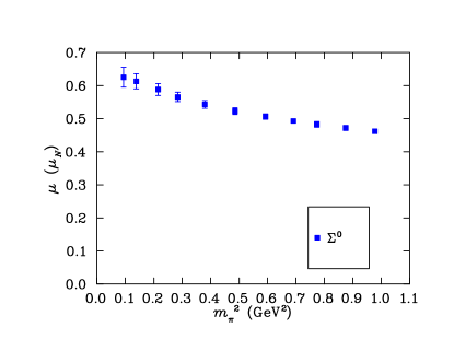
Figure 25: Magnetic moment of $\Sigma^{0}$.

Figure 26: Magnetic moments of the proton and $\Sigma^{+}$. The $\Sigma^{+}$ moments are offset to the right for clarity.

Figure 25 presents results for the $\Sigma^{0}$ baryon where chiral curvature is anticipated to be small. However, a comparison of $p$ and $\Sigma^{+}$ magnetic moments provides a favourable opportunity to observe chiral curvature. The proton has a strong negative coupling to the pion channel, predicting curvature towards positive values as the chiral limit is approached. This contrasts the $\Sigma^{+}$ where the strong coupling is to the energetically unfavourable $\Xi K$ channel suggesting a more linear approach to the chiral limit.

Figure 26 depicts the variation of these moments with quark mass. These results are highly correlated and therefore the enhancement of the magnetic moment of the proton over the $\Sigma^{+}$ provides significant evidence of chiral non-analytic behaviour in accord with the LNA predictions of chiral perturbation theory. The strong correlation of these results is evident in the $SU(3)$ flavour-symmetric point at $m_{\pi}^{2}\simeq 0.5\ {\rm GeV}^{2}$ where the results are identical.

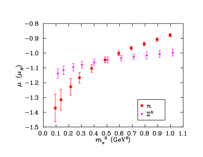
Figure 27: Magnetic moments of the neutron and $\Xi^{0}$. $\Xi^{0}$ moments are offset to the right for clarity.

Figure 27 reports the magnetic moments of the neutron and $\Xi^{0}$. The neutron provides a favourable case for the observation of chiral curvature associated with the pion channel. Similarly the $\Xi^{0}$ has significant strength in the energetically favoured $\Sigma K$ channel. In both cases the chiral coefficient, $\chi$ is positive, predicting curvature towards negative values as the chiral limit is approached. These predictions are in accord with the observations of Fig. 27.

In summary, we have performed an unprecedented exploration of the light quark-mass properties of octet-baryon magnetic moments in quenched QCD. Figure 28 presents our results in the context of recent state of the art results from lattice QCD Leinweber:1990dv ; Wilcox:1991cq ; Gockeler:2003ay . The precision afforded by 400, $20^{3}\times 40$ lattices and the efficient access to the chiral regime enabled by our use of the FLIC fermion action is clear. In every case, the LNA curvature predicted by chiral perturbation theory is manifest in our results.

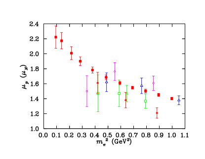
Figure 28: Proton magnetic moment in nuclear magnetons is compared from a variety of lattice simulations. The solid squares indicate our current lattice QCD results with FLIC fermions. The stars indicate the early lattice results of Ref. Leinweber:1990dv . The crosses (only one point) indicate the results of Ref. Wilcox:1991cq . The open symbols describe the QCDSF collaboration results Gockeler:2003ay . Open squares indicate results with $\beta=6.0$, open triangles indicate those with $\beta=6.2$ while the open diamonds indicate their results with $\beta=6.4$.

V.2.4 Ratio of $\mu_{\Xi^{-}}$ to $\mu_{\Lambda}$

The experimentally measured value of magnetic moment of $\Xi^{-}$ is $-0.651\pm 0.003\mu_{N}$ and that of $\Lambda$ is $-0.613\pm 0.004\mu_{N}$, making their ratio greater than 1 at $1.062\pm 0.012$. This has presented a long-standing problem to constituent quark models which predict the magnetic moment ratio, $\Xi^{-}/\Lambda^{0}$, to be less than one.

In the simple $SU(6)$ spin-flavour quark model, the magnetic moment of $\Xi^{-}$ is

$$\mu_{\Xi^{-}}=\frac{4}{3}\mu_{s}-\frac{1}{3}\mu_{d}\,,$$ (55)

where $\mu_{s}$ and $\mu_{d}$ are the magnetic moments of the constituent $s$ and $d$ quarks respectively. Since the $u$-$d$ pair in $\Lambda$ forms a spin-$0$ state, the magnetic moment of the $\Lambda$ has a sole contribution from the $s$ quark

$$\mu_{\Lambda}=\mu_{s}\,.$$ (56)

Taking the ratio yields

$$\frac{\mu_{\Xi^{-}}}{\mu_{\Lambda}}=\frac{4}{3}-\frac{1}{3}\frac{\mu_{d}}{\mu_{s}}\,.$$ (57)

Now since, the magnetic moment of a charged Dirac particle goes inversely as its mass, and since the $s$ and $d$ quarks have identical charge, the ratio may be written

$$\frac{\mu_{\Xi^{-}}}{\mu_{\Lambda}}=\frac{4}{3}-\frac{1}{3}\frac{m_{s}}{m_{d}}\,,$$ (58)

where $m_{d}$ and $m_{s}$ are the constituent masses of the $d$ and $s$ quarks respectively. Given that $m_{s}>m_{d}$ it is inescapable that this ratio is less than 1 in the simple quark model. Indeed, the accepted values of $d$ and $s$ constituent quark masses place this ratio at $0.836$.

Figure 29 shows the ${\mu_{\Xi^{-}}}/{\mu_{\Lambda}}$ ratio as a function of quark mass as observed in our quenched lattice calculations. Remarkably, the ratio is greater than one at all quark masses.

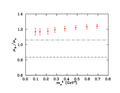
Figure 29: Magnetic moment ratio $\mu_{\Xi^{-}}/\mu_{\Lambda}$ as calculated in quenched QCD. The simple quark model results of 0.836 is illustrated by the dashed line while the experimental value of the ratio is indicated by the dot-dash line.

There are two important aspects of our previous discussion that give rise to a result exceeding 1. First, as illustrated in Fig. 20, we have found that the singly represented quarks give a contribution to the magnetic moment that is much smaller in magnitude than that of the $SU(6)$ quark model prediction. This gives rise to a 40% reduction in the contribution of the second term of Eq. (58).

While this is sufficient to correct the ratio to $\sim 1$, there is a second effect. Namely, the light quark sector makes a non-trivial contribution to the $\Lambda$ magnetic moment. As illustrated in Fig. 21, this contribution is positive for unit charge quarks. Since the net charge of the $u$-$d$ sector is $+1/3$, the contribution of the $s$ quark in $\Lambda^{0}$ must have a negative value whose magnitude exceeds the observed $\Lambda$ moment. And this is seen in Fig. 22. There, chiral curvature in $s_{\Lambda}$ makes the ratio of magnetic moment contributions $s_{\Lambda}/s_{\Xi}\sim 3/2$ as opposed to the $SU(6)$ suggestion of 4/3. This resolves the long-standing discrepancy.

V.3 Magnetic radii

Using the values for the magnetic moments obtained by scaling the individual quark sector contributions to $Q^{2}=0$, and our values for the form factors at finite $Q^{2}$, magnetic radii may be determined in exactly the same fashion as the electric radii.

Analogous to the charge radius, we adopt a dipole form for the $Q^{2}$ dependence and define the magnetic radius as

$$\frac{\langle r_{M}^{2}\rangle}{{\cal G}_{M}(0)}={12\over Q^{2}}\left(\sqrt{{\cal G}_{M}(0)\over{\cal G}_{M}(Q^{2})}-1\right).\quad$$ (59)

The magnetic radii, ${\langle r_{M}^{2}\rangle}/{{\cal G}_{M}(0)}$, are tabulated in Table 20. Figures 30 through 33 display the variation of the magnetic radii with $m_{\pi}^{2}$ for the octet baryons.

Table 20: Magnetic radii ${\langle r_{M}^{2}\rangle}/{{\cal G}_{M}(0)}$ of the octet baryons in ${\rm fm}^{2}$ for various $m_{\pi}^{2}$ in ${\rm GeV}^{2}$.

$m_{\pi}^{2}$	$p$	$n$	$\Sigma^{+}$	$\Sigma^{0}$	$\Sigma^{-}$	$\Lambda$	$\Xi^{0}$	$\Xi^{-}$
$0.9972(55)$	$0.241(7)$	$0.240(6)$	$0.254(9)$	$0.264(9)$	$0.236(10)$	$0.328(14)$	$0.298(13)$	$0.337(16)$
$0.8947(54)$	$0.255(8)$	$0.252(7)$	$0.265(10)$	$0.273(9)$	$0.252(10)$	$0.328(14)$	$0.302(13)$	$0.335(17)$
$0.7931(53)$	$0.269(9)$	$0.266(9)$	$0.278(10)$	$0.283(10)$	$0.269(12)$	$0.328(16)$	$0.306(13)$	$0.334(17)$
$0.6910(35)$	$0.286(9)$	$0.283(8)$	$0.292(10)$	$0.294(9)$	$0.287(11)$	$0.339(14)$	$0.314(12)$	$0.340(14)$
$0.5925(33)$	$0.305(10)$	$0.301(10)$	$0.308(11)$	$0.308(11)$	$0.309(12)$	$0.340(15)$	$0.319(12)$	$0.339(15)$
$0.4854(31)$	$0.330(14)$	$0.326(13)$	$0.330(14)$	$0.326(13)$	$0.337(15)$	$0.342(17)$	$0.326(13)$	$0.337(15)$
$0.3795(31)$	$0.356(17)$	$0.351(16)$	$0.352(16)$	$0.344(15)$	$0.365(18)$	$0.343(18)$	$0.334(14)$	$0.334(16)$
$0.2839(33)$	$0.387(21)$	$0.382(21)$	$0.377(19)$	$0.364(18)$	$0.396(22)$	$0.348(20)$	$0.343(16)$	$0.332(16)$
$0.2153(35)$	$0.415(27)$	$0.413(28)$	$0.395(24)$	$0.380(22)$	$0.418(27)$	$0.353(22)$	$0.352(17)$	$0.330(16)$
$0.1384(43)$	$0.438(31)$	$0.439(32)$	$0.428(32)$	$0.407(29)$	$0.462(36)$	$0.351(22)$	$0.365(19)$	$0.328(17)$
$0.0939(44)$	$0.470(48)$	$0.478(50)$	$0.446(42)$	$0.423(38)$	$0.483(49)$	$0.347(24)$	$0.384(22)$	$0.336(18)$

Figure 30: Magnetic radii of the proton and $\Sigma^{+}$. The latter are shifted right for clarity.

Figure 30 depicts the magnetic radii of the proton and $\Sigma^{+}$ as a function of input quark mass. The somewhat subtle differences have a simple explanation in terms of the more localised strange quark in $\Sigma$.

In the proton, the long-range nature of the light-quark distributions means that their contributions to the magnetic form factor reduce quickly for increasing momentum transfers. In the case of $\Sigma^{+}$, which has a broadly distributed $u$ quark distribution and a narrowly distributed $s$ quark distribution, the reduction in magnitude of the form factor is less. Here, the $s$-quark distribution contributes positively and remains relatively invariant with increased resolution. Thus the $\Sigma^{+}$ has a larger form factor than the proton at finite $Q^{2}$ and hence a smaller magnetic radius.

Figure 31 reports the magnetic radii of the neutron and $\Xi^{0}$. Following a similar argument as above, the neutron is expected to have a larger magnetic radius than the $\Xi^{0}$, and this is confirmed in the plot.

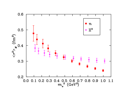
Figure 31: Magnetic radii of the neutron and $\Xi^{0}$. The latter are shifted to the right for clarity.

Figure 32 illustrates the magnetic radii of $\Lambda$ and $\Sigma^{0}$ as a function of the input quark mass. In $\Lambda$, most of the magnetic moment has its origin in the $s$ quark and therefore the magnetic radius will be relatively small. In the $\Sigma^{0}$ the $u$-$d$ sector is a major contributor to the form factor. As a result, the form factor reduces more at finite momentum transfer, which in turn implies that the magnetic radius of the $\Sigma^{0}$ will be relatively large.

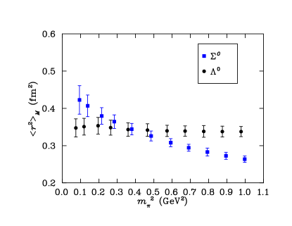
Figure 32: Magnetic radii of $\Sigma^{0}$ and $\Lambda$. The latter are shifted left for clarity.

Figure 33: Magnetic radii of $\Sigma^{+}$, $\Sigma^{-}$ and $\Xi^{-}$. Results for $\Sigma^{+}$ and $\Xi^{-}$ are offset left and right respectively for clarity.

Figure 33 illustrates the magnetic radii of $\Sigma^{-}$, $\Sigma^{+}$ and $\Xi^{-}$. $\Sigma^{+}$ is replotted here to facilitate comparison with the other two members of the baryon octet.

$\Sigma^{-}$ has the largest magnetic radius among the octet baryons and this is to be expected based on our considerations of the origin of the baryon magnetic moment. Here, the doubly represented $d$ quark contributes to the total baryon form factor with the same sign, whereas the strange sector acts to reduce the magnitude of the total form factor. Upon increasing the momentum transfer resolution, the $d$-sector is reduced dramatically whereas the strange sector, acting to reduce the total form factor, is relatively preserved. this gives rise to a large drop in the total form factor at finite $Q^{2}$ and thus a large magnetic radius.

On the other hand, the singly represented $d$ quark in the $\Xi^{-}$ makes only a small contribution to the $\Xi^{-}$ form factor, and therefore the magnetic radius reflects the small distribution of the strange quark.

VI SUMMARY

We have presented an extensive investigation of the electromagnetic properties of octet baryons in quenched QCD. The development of the ${\cal O}(a)$-improved FLIC fermion action has been central to enabling this study. The FLIC fermion operator is an efficient nearest-neighbour fermion operator with excellent scaling properties Zanotti:2004dr . The vastly improved chiral properties of this operator FLIClqm enables the exploration of the electromagnetic form factors at quark masses significantly lighter than those investigated in the past. The unprecedented nature of our quark masses is illustrated in Figs. 16 and 28 for the proton charge radii and magnetic moments, respectively.

Central to our discussion of the results is the search for evidence of chiral non-analytic behaviour as predicted by chiral perturbation theory. We have discovered that all baryons having non-vanishing, energetically-favourable couplings to virtual meson-baryon transitions tend to be broader than those which do not. This qualitative realisation provides a simple explanation for the patterns revealed in our quenched-QCD simulations.

Of particular interest is the environmental isospin dependence of the strange quark distributions in $\Lambda^{0}$ and $\Sigma^{0}$. When the environmental quarks are in an isospin-0 state in the $\Lambda$, the strange quark distribution is broad. On the other hand, when the environmental quarks are in an isospin-1 state in $\Sigma$ baryons, the distribution radius is significantly smaller.

Still, evidence of chiral curvature on our large-volume lattice is rather subtle in general and absent in the exceptional case of the singly-represented quark in the neutron or $\Xi$. In this case, the chiral loop effects act to oppose the Compton broadening of the distribution. However, it is thought that the restriction of momenta to discrete values on the finite-volume lattice prevents the build up of strength in the loop integral sufficient to counter the natural broadening of the distribution as the quark becomes light. It will be interesting to explore this quantitatively in finite-volume chiral effective field theory.

In contrast, chiral curvature is evident in the quark-sector contributions to baryon magnetic moments. In every case, the curvature predicted by chiral perturbation theory is manifest in our results. Of particular mention is the comparison of the $u$-quark contribution to the proton and $\Sigma^{+}$ illustrated in Figs. 17 and 18. The environment sensitivity of the $s$ quark in $\Lambda^{0}$ depicted in Fig. 22 is particularly robust.

We find it remarkable that the leading non-analytic features of chiral perturbation theory are observed in our simulation results. Naively, one might have expected a non-trivial role for the higher order terms of the chiral expansion which might have acted to hide the leading behaviour. However, the smooth and slow variation of our simulation results indicate that these higher order terms must sum to provide only a small correction to the leading behaviour. These observations indicate that regularisations of chiral effective field theory which resum the chiral expansion at each order, to ensure that higher order terms sum to only small corrections, will be effective in performing quantitative extrapolations to the physical point. Indeed work in this direction Young:2004tb ; Leinweber:2004tc ; Leinweber:2006ug has been very successful.

Comparison of our quenched QCD results with experiment is not as interesting. The chiral physics of quenched QCD differs from the correct chiral physics of full QCD and our results explore sufficiently light quark masses to reveal these discrepancies. The simulation results do not agree with experiment, particularly for light quark baryons where chiral physics makes significant contributions. However, methods have been discovered for quantitatively estimating the corrections to be encountered in simulating full QCD and we refer the interested reader to Refs. Young:2004tb ; Leinweber:2004tc ; Leinweber:2006ug for further discussion.

In future simulations it will be interesting to explore the utility of boundary conditions which allow access to arbitrarily small momentum transfers, providing opportunities to map out hadron form factors in detail. Similarly, by calculating near $Q^{2}=0$ one would have more direct access to the magnetic moment. Nevertheless, such boundary conditions cannot be seen to substitute for larger volume lattices, as the discretisation of the momenta due to the finite volume of the lattice acts to suppress chiral non-analytic behaviour. Only with increasing lattice volumes will the continuous momentum of chiral loops be approximated well on the lattice.

- (1) W. Wilcox and R. M. Woloshyn, Phys. Rev. Lett. 54, 2653 (1985); R. M. Woloshyn and A. M. Kobos, Phys. Rev. D 33, 222 (1986); R. M. Woloshyn, Phys. Rev. D 34, 605 (1986); T. Draper, R. M. Woloshyn, W. Wilcox and K. F. Liu, Nucl. Phys. B 318, 319 (1989).
- (2) G. Martinelli and C. T. Sachrajda, Nucl. Phys. B 306, 865 (1988); G. Martinelli and C. T. Sachrajda, Nucl. Phys. B 316, 355 (1989).
- (3) T. Draper, R. M. Woloshyn and K. F. Liu, Phys. Lett. B 234, 121 (1990).
- (4) D. B. Leinweber, R. M. Woloshyn and T. Draper, Phys. Rev. D 43 (1991) 1659.
- (5) W. Wilcox, T. Draper and K. F. Liu, Phys. Rev. D 46, 1109 (1992) [arXiv:hep-lat/9205015].
- (6) D. B. Leinweber, T. Draper and R. M. Woloshyn, Phys. Rev. D 46, 3067 (1992) [arXiv:hep-lat/9208025].
- (7) D. B. Leinweber, T. Draper and R. M. Woloshyn, Phys. Rev. D 48, 2230 (1993) [arXiv:hep-lat/9212016].
- (8) J. M. Zanotti, S. Boinepalli, D. B. Leinweber, A. G. Williams and J. B. Zhang, Nucl. Phys. Proc. Suppl. 128, 233 (2004) [arXiv:hep-lat/0401029].
- (9) D. B. Leinweber et al., Phys. Rev. Lett. 94, 212001 (2005) [arXiv:hep-lat/0406002].
- (10) D. B. Leinweber, et al., Eur. Phys. J. A 24S2, 79 (2005) [arXiv:hep-lat/0502004].
- (11) D. B. Leinweber et al., arXiv:hep-lat/0601025.
- (12) M. Gockeler et al., [QCDSF Collaboration], Phys. Rev. D 71, 034508 (2005) [arXiv:hep-lat/0303019].
- (13) R. G. Edwards et al. [LHPC Collaboration], PoS LAT2005, 056 (2005) [arXiv:hep-lat/0509185].
- (14) D. B. Leinweber, Phys. Rev. D 69, 014005 (2004) [arXiv:hep-lat/0211017].
- (15) M. J. Savage, Nucl. Phys. A 700, 359 (2002) [nucl-th/0107038].
- (16) N. Mathur and S. J. Dong, Nucl. Phys. Proc. Suppl. 94, 311 (2001) [arXiv:hep-lat/0011015]; S. J. Dong, et al., Phys. Rev. D58, 074504 (1998) [arXiv:hep-ph/9712483].
- (17) R. Lewis, W. Wilcox and R. M. Woloshyn, Phys. Rev. D 67, 013003 (2003) [arXiv:hep-ph/0210064].
- (18) J. Foley, K. Jimmy Juge, A. O’Cais, M. Peardon, S. M. Ryan and J. I. Skullerud, Comput. Phys. Commun. 172, 145 (2005) [arXiv:hep-lat/0505023].
- (19) D. B. Leinweber, Phys. Rev. D 45, 252 (1992).
- (20) D. B. Leinweber, Phys. Rev. D 47, 5096 (1993) [arXiv:hep-ph/9302266].
- (21) D. B. Leinweber and A. W. Thomas, Phys. Rev. D 62, 074505 (2000) [arXiv:hep-lat/9912052].
- (22) M. Luscher and P. Weisz, Commun. Math. Phys. 97, 59 (1985) [ibid. 98, 433 (1985)].
- (23) R. Sommer, Nucl. Phys. B 411, 839 (1994) [arXiv:hep-lat/9310022].
- (24) J.M. Zanotti et al., Phys. Rev. D 60 (2002) 074507 [arXiv:hep-lat/0110216]; Nucl.Phys.Proc.Suppl. 109 101 (2002) [arXiv:hep-lat/0201004].
- (25) S. O. Bilson-Thompson, et al., Annals Phys. 304, 1 (2003) [arXiv:hep-lat/0203008].
- (26) J.J. Sakurai, “Advanced Quantum Mechanics” (Addison-Wesley, 1982).
- (27) J. M. Zanotti, B. Lasscock, D. B. Leinweber and A. G. Williams, Phys. Rev. D 71, 034510 (2005) [arXiv:hep-lat/0405015].
- (28) S. Boinepalli, W. Kamleh, D. B. Leinweber, A. G. Williams and J. M. Zanotti, Phys. Lett. B 616, 196 (2005) [arXiv:hep-lat/0405026].
- (29) S. Gusken, Nucl. Phys. Proc. Suppl. 17, 361 (1990).
- (30) J. M. Zanotti, et al., Phys. Rev. D 68, 054506 (2003) [arXiv:hep-lat/0304001].
- (31) G. Martinelli, C. T. Sachrajda and A. Vladikas, Nucl. Phys. B 358 (1991) 212.
- (32) T. Draper, R. M. Woloshyn, W. Wilcox and K. F. Liu, Nucl. Phys. Proc. Suppl. 9, 175 (1989).
- (33) W. Melnitchouk et al., Phys. Rev. D 67, 114506 (2003) [arXiv:hep-lat/0202022].
- (34) D. B. Leinweber, W. Melnitchouk, D. G. Richards, A. G. Williams and J. M. Zanotti, Lect. Notes Phys. 663, 71 (2005) [arXiv:nucl-th/0406032].
- (35) D. B. Leinweber and T. D. Cohen Phys. Rev. D 47 (1993) 2147. [arXiv:hep-lat/9211058].
- (36) D. Arndt and B. C. Tiburzi Phys. Rev. D 68 (2003) 094501. [arXiv:hep-lat/0307003].
- (37) S. Boinepalli, et al., [CSSM Lattice Collaboration], in preparation.
- (38) R. D. Young, D. B. Leinweber and A. W. Thomas, Phys. Rev. D 71, 014001 (2005) [arXiv:hep-lat/0406001].