Dynamical QCD simulations on anisotropic lattices

Abstract

The simulation of QCD on dynamical ($N_{f}=2$) anisotropic lattices is described. A method for nonperturbative renormalisation of the parameters in the anisotropic gauge and quark actions is presented. The precision with which this tuning can be carried out is determined in dynamical simulations on $8^{3}\times 48$ and $8^{3}\times 80$ lattices.

I Introduction

The advantages of simulations with anisotropic lattices are well understood and the method has been used for precision determinations of an extensive range of quantities in the quenched approximation to QCD Karsch:1982ve ; Manke:1998qc ; Morningstar:1999rf ; Asakawa:2003re ; Hashimoto:2003fs ; Ishii:2005vc . In general a 3+1 anisotropy is employed where the lattice spacing in the temporal direction, $a_{t}$, is made fine whilst keeping the spatial lattice spacing $a_{s}$ relatively coarse. The advantages of this approach are two-fold. The improved resolution in the temporal direction means that states whose signal to noise ratio falls rapidly can be more reliably determined. The high computational cost of this improvement is offset by savings in the coarse spatial directions.

The isotropic lattice (whose spacing in the four space-time directions is $a_{x}=a_{y}=a_{z}=a_{t}\equiv a$) regulates QCD in a way that breaks the continuous Euclidean symmetry down to the finite group of rotations of the hypercube. Luckily the relevant operators that transform trivially under these two groups are the same and so there is no renormalisation of the speed of light on the isotropic lattice. Once an explicitly anisotropic lattice action is introduced with $a_{x}=a_{y}=a_{z}\equiv a_{s}$ and $a_{t}\neq a_{s}$, the rotational symmetry of the theory is the cubic point group. For the gluons, there are now two distinct operators not related by rotations at dimension four: $\left\{\mbox{Tr }E^{2},\mbox{Tr }B^{2}\right\}$; while for the quarks the set of dimension four operators $\left\{\bar{\psi}\;/D\psi,\;m\bar{\psi}\psi\right\}$ grows to a set with three members: $\left\{\bar{\psi}\gamma_{i}D_{i}\psi,\;\bar{\psi}\gamma_{0}D_{0}\psi,\;m\bar{\psi}\psi\right\}$. As a result, two new parameters appear in the action, and for the continuum limit to represent QCD these parameters must be determined such that a physical probe of the vacuum at scales well below the cut-off appears to have full Euclidean symmetry. The nonperturbative determination of these extra action parameters is the subject of the present paper.

In quenched QCD the anisotropy in the gauge sector, $\xi_{g}$, and the quark sector, $\xi_{q}$, can be tuned independently and post hoc using two separate criteria. The precision and mass-dependence of the determination of $\xi_{q}$ was investigated for the action we use in Ref. Foley:2004jf . It was found that this parameter could be determined at the percent level from the energy-momentum dispersion relation. The mass dependence was found to be mild for quark masses in the range $m_{s}\leq m_{q}\leq m_{c}$ when the tuning was carried out at the strange quark mass, $m_{s}$. In Refs. Klassen:1998ua ; Alford:2000an , a determination of the gluonic parameter was made to similar precision.

We would like to use anisotropic lattices in simulations with $N_{f}=2$ for realistic phenomenologically-relevant calculations. In dynamical QCD the tuning procedure becomes more complicated because of the interplay between the quark and gluon sectors and the parameters must be simultaneously determined. There are several issues to resolve. Firstly, can this simultaneous tuning be accomplished; secondly, to what precision is the renormalised anisotropy determined; and thirdly, what is the mass-dependence of the renormalised anisotropy. Here we will focus on the first two issues, and leave the question of the mass dependence to a later study.

The paper is organised as follows. Section II gives the details of the gauge and quark actions used in this investigation. Section III describes the tuning methodology and is followed in Section IV by the results for the values of the tuned bare (input) parameters $\xi^{0}_{g}$ and $\xi^{0}_{q}$. Section V contains our conclusions and future plans.

II The action and parameters

We begin with a brief description of the anisotropic action used in this study. The details of the tuning procedure described in Section III do not depend on the specific action used. Further description of the action can be found in Foley:2004jf where the tuning for the same action in the quenched approximation was discussed.

The gauge action is a two-plaquette Symanzik-improved action Morningstar:1999dh previously developed for high-precision glueball studies and given by

$$\begin{split}S_{G}=&\frac{\beta}{\xi^{0}_{g}}\left\{\frac{5(1+\omega)}{3u^{4}_{s}}\Omega_{s}-\frac{5\omega}{3u^{8}_{s}}\Omega^{(2t)}_{s}-\frac{1}{12u^{6}_{s}}\Omega^{(R)}_{s}\right\}\\ &+\beta\xi^{0}_{g}\left\{\frac{4}{3u^{2}_{s}u^{2}_{t}}\Omega_{t}-\frac{1}{12u^{4}_{s}u^{2}_{t}}\Omega^{(R)}_{t}\right\},\end{split}$$ (1)

where $\Omega_{s}$ and $\Omega_{t}$ are spatial and temporal plaquettes. $\Omega_{s}^{R}$ and $\Omega_{t}^{R}$ are $2\times 1$ rectangles in the $(i,j)$ and $(i,t)$ planes respectively. $\Omega_{s}^{2t}$ is constructed from two spatial plaquettes separated by a single temporal link. $u_{s}$ and $u_{t}$ are the mean spatial and temporal gauge link values respectively. The action has leading discretisation errors of ${\cal O}(a^{3}_{s},a_{t},\alpha_{s}a_{s})$.

For fermions an action specifically designed for large anisotropies is used. The usual Wilson term removes doublers in the temporal direction whereas spatial doublers are removed by the addition of a Hamber–Wu term. The action has been described in detail in Ref. Foley:2004jf and has leading classical discretisation errors of ${\cal O}(a_{t}m_{q})$. In terms of continuum operators, it can be written

$$S=\bar{\psi}(/D+m_{0})\psi-\frac{ra_{t}}{2}\bar{\psi}\left(D_{0}^{2}\right)\psi+sa^{3}_{s}\bar{\psi}\sum_{i}D_{i}^{4}\psi,$$ (2)

which highlights the different treatment of temporal and spatial directions. $r$ is the usual Wilson coefficient which is applied in the temporal direction only in this action and is set to unity. The analagous parameter in the spatial directions is $s$, which parameterises a term that is irrelevant in the continuum limit. A precise tuning of this parameter is not necessary: in practice we choose $s=1/8$, so that the energy of a propagating quark at tree level increases monotonically across the Brillouin zone. Stout-link smearing Morningstar:2003gk was used for the gauge fields in the fermion matrix. Two stoutening iterations were used, with a parameter $\rho=0.22$. This was fixed for all simulations, and chosen to approximately maximise the expectation value of the spatial plaquette on the stout links.

This study was carried out on $8^{3}\times 48$ and $8^{3}\times 80$ anisotropic lattices with a spatial lattice spacing $a_{s}\approx 0.2$fm and a target anisotropy $\xi=6$. The bare sea quark mass was set to $a_{t}m_{q}=-0.057$ in all runs. A set of gauge configurations, distributed across ten independent Markov chains, was generated for each set of input parameters ($\xi^{0}_{g}$,$\xi^{0}_{q}$). Valence quark propagators were generated with the same mass as the sea quarks.

To determine the statistical uncertainties, 1000 bootstrapped sets of configurations were taken and analysis was done on these bootstrapped sets. Both point and all-to-all propagators were used. Some preliminary results using point propagators on $8^{3}\times 48$ lattices were presented in Ref. Morrin:2005tc .

III Methodology

The bare parameters, $\xi^{0}_{g}$ and $\xi^{0}_{q}$, are renormalised by demanding that physical probes exhibit euclidean symmetry. In principle, any physical quantity can be used; however, it should be easily determined to high precision. In this study we have used the sideways potential and the pion energy-momentum dispersion relation for the gauge and fermion sectors respectively.

The gauge anisotropy $\xi_{g}$ is determined from the interquark potential Klassen:1998ua ; Alford:2000an . The static source propagation is chosen to be along a coarse direction allowing the sources to be separated along both course and fine axes. The potential is determined at the same physical distance for these two cases. The input anisotropy is constrained so that the two calculations yield the same value of the potential, $V_{s}(x)=V_{t}(t/\xi)$ for a target anisotropy $\xi$. For a given input anisotropy $\xi^{0}_{g}$ and target anisotropy $\xi$ we can determine the mismatch parameter $c_{g}=V_{s}(x)/V_{t}(t/\xi)$. If $x$ is in the régime where the potential is nearly linear, the mismatch parameter is approximately related to the actual gauge anisotropy, $c_{g}\approx\xi_{g}/\xi$.

The quark anisotropy can be determined from the pseudoscalar dispersion relation. The anisotropy is inversely proportional to the square root of the slope of the dispersion relation and demanding a relativistic energy-momentum relation imposes a renormalisation condition on the bare parameter $\xi^{0}_{q}$. The ground state energy $E_{0}$ was determined for a range of momenta, $n^{2}\in\{0,1,2,3,4,5,6\}$, where $p_{n}=\frac{2\pi n}{La_{s}}$ and we average over equivalent momentum values. The two-point correlator data were modelled with single exponentials and a $\chi^{2}$-minimisation was used to determine the best-fit ground state. These values were used to generate an energy-momentum dispersion relation.

In the quenched approximation this procedure is relatively easy since $\xi^{0}_{g}$ and $\xi^{0}_{q}$ can be determined independently. For dynamical simulations it is no longer possible to simply fix $\xi^{0}_{g}$ and then tune $\xi^{0}_{q}$ to a consistent value, since changing $\xi^{0}_{q}$ will affect the measurement of $\xi_{g}$. Explicitly, changing the value of $\xi^{0}_{q}$ necessitates a regeneration of the background fields with the new value of $\xi^{0}_{q}$ which in turn will change the measured anisotropy $\xi_{g}$ of the background fields. The solution to this problem is a simultaneous two-dimensional tuning procedure Peardon:2002sd .

A linear dependence on the parameters $\xi^{0}_{g}$ and $\xi^{0}_{g}$ was assumed for a small region. Three initial sets of configurations were generated and the renormalised anisotropy was determined. Planes were defined for both output values of $\xi_{g}$ and $\xi_{q}$ i.e. values $\alpha,\beta,\gamma$ were found to satisfy $\xi_{a}=\alpha_{a}\xi^{0}_{g}+\beta_{a}\xi^{0}_{q}+\gamma_{a}$ for the renormalised anisotropy $\xi_{a},a=g,q$ measured for each input $(\xi^{0}_{q},\xi^{0}_{g})$. The intersection of these planes with the required (target) output value yields the tuned point. The statistical uncertainties were determined using bootstrap resampling, with a common bootstrap ensemble used for all measurements. When more than three simulation points were available a plane was defined using a constrained-$\chi^{2}$ fit.

All observables were estimated using the Monte Carlo method. An ensemble of 250 gauge field configurations divided across 10 Markov chains was generated using the Hybrid Monte Carlo (HMC) algorithm Duane:1987de . Approximately 5000 CPU hours were needed in order to generate each set of configurations. The HMC algorithm can be used for these simulations without modification. One observation serves to improve performance, however. HMC adds a set of momentum variables conjugate to the gauge fields, but each conjugate momentum can be added with a different gaussian variance without changing the validity of the method. In isotropic simulations this is not a useful property, and all momentum co-ordinates are chosen to have unit variance. For the anisotropic lattice, the temporal and spatial gauge fields have different interactions, and different momenta become useful. If the HMC hamiltonian is

$${\cal H}=\sum_{x}\left(\frac{1}{2\mu_{t}^{2}}\mbox{Tr }P_{0}^{2}(x)+\sum_{i=1}^{3}\frac{1}{2}\mbox{Tr }P_{i}^{2}(x)\right)+S[U],$$ (3)

an extra tunable parameter, $\mu_{t}$ (the variance of the temporal link momenta), has been added to the algorithm which can be used to optimise acceptance by the Metropolis test. This is equivalent to using two distinct integration step-sizes for the spatial and temporal degrees of freedom. Some brief numerical experiments suggest that a temporal leap-frog step-size smaller by a factor $\xi$ is close to optimal, and this is borne out by considerations of free field theory.

IV Results

Run	1	2	3	4	5
$\beta$	1.51	1.528	1.514	1.544	1.522
$\xi_{q}^{0}$	6.0	7.5	7.5	8.72	8.83
$\xi_{g}^{0}$	8.0	7.0	8.0	6.65	7.44

Table 1: Input parameters for the five dynamical simulations performed in this tuning procedure. The bare quark mass is $a_{t}m_{q}=-0.057$ for all runs.

The input anisotropy parameters used are given in Table 1. We started by choosing three points (Runs 1–3) in the $(\xi^{0}_{g},\xi^{0}_{q})$ plane, and generated configurations at two further points as a result of the tuning procedure. The final tuning was performed on $8^{3}\times 80$ lattices, using data from runs 1, 4 and 5 as these spanned the largest area of the plane.

IV.1 Interquark Potential

The gluon anisotropy is determined from the static quark potential at a selected distance $R$. In practice this is done by determining the effective energy for the static quark–antiquark configuration at separation $R$ at some time $T$. It is then important to choose values for $R$ and $T$ where the potential is well determined and the value obtained for $c_{g}$ is stable with respect to small variations in $R$ and $T$. The same values for $R$ and $T$ must then be used for all runs in order to have a consistent procedure.

Table 2 shows $c_{g}$ for different $R$ and $T$, on the $8^{3}\times 80$ lattices. We see that the values are generally quite consistent for each run. Looking more closely at the effective potential for each $R$ as a function of $T$, we find that it has not yet reached a plateau at $T=1$, while the value for $T=3$ is consistent within errors with that for $T=2$. We choose $(T,R)=(2,3)$ as our optimal parameters, since this yields reasonably small statistical errors, while $R$ is large enough to be in the linear régime.

	$c_{g}=V_{s}(x)/V_{t}(t/\xi)$ at different (T,R)
Run	(1,3)	(1,4)	(2,3)	(2,4)	(3,3)	(3,4)
1	0.972(2)	0.959(3)	0.972(7)	0.965(13)	0.991(25)	1.13(8)
4	0.951(2)	0.941(4)	0.945(8)	0.926(18)	0.942(34)	0.89(9)
5	0.994(2)	0.990(3)	0.991(7)	0.998(13)	0.965(25)	1.01(7)

Table 2: The gluon anisotropy parameter $c_{g}$ for different separations, $R$ and times, $T$. The final results were determined from data at $T=2$ and $R=3$.

IV.2 Dispersion relations

Pseudoscalar meson correlators were computed using traditional point propagators as well as all-to-all propagators Foley:2005ac with time and colour dilution and no eigenvectors.

To determine optimal fit ranges for exponential fits to the correlator data, sliding window ($t_{\text{min}}$) plots were used: the correlation function was fitted in a range from $t_{\text{min}}$ to $t_{\text{max}}$ where $t_{\text{max}}$ was fixed to the largest value compatible with a good fit, and $t_{\text{min}}$ was varied. An example of such a plot is given in Fig. 1. The fit range was chosen so the fit would be stable with respect to small variations in $t_{\text{min}}$. The same fit ranges and smearing parameters were chosen for all simulation points in order to obtain a consistent determination of the dispersion relation. The final fit ranges are given in Table 3.

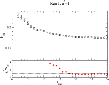
Figure 1: A typical $t_{\text{min}}$ plot, showing the energy for momentum $n^{2}=1$ on run 1, $8^{3}\times 80$ lattices from fits to time ranges $t_{\text{max}}=40$ for various $t_{\text{min}}$. A stable ground state energy determination, with a good $\chi^{2}$, is achieved for $22\leq t_{\text{min}}\leq 30$.

$n^{2}$	$t_{\text{min}}$	$t_{\text{max}}$
0	25	40
1	24	40
2	21	40
3	19	40

Table 3: Fit ranges.

In our initial analysis data from a $8^{3}\times 48$ lattice were used. However, a reliable extraction of the ground state energy proved difficult. In particular, it was observed that the energy either did not reach a plateau until near the end of the lattice or did not plateau at all. To resolve this problem the simulation was repeated on a longer, $8^{3}\times 80$ lattice. An immediate improvement in the quality of the fits was observed. The ground state energy was determined from fits over at least 15 timeslices and was stable with respect to changes in $t_{\text{min}}$. The effect of the longer lattice is illustrated in Figure 2. This plot also compares simulations using point and all-to-all propagators. The all-to-all propagators lead to improved precision in the fitted energies. The central values are in agreement with the energies determined using point propagators but the statistical error is smaller.

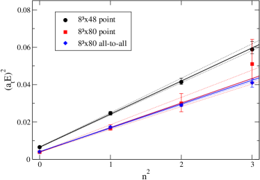
Figure 2: A comparison of the dispersion relations determined from an $8^{3}\times 48$ lattice and an $8^{3}\times 80$ lattice. The solid lines are the best fits and the dotted lines are the 68% confidence levels. The figure also shows a comparison of all-to-all propagators and point propagators on the same (longer) lattice. The plot shows that the ground state energies have not reached a plateau on the shorter lattice. On the longer lattice the all-to-all and point data agree, while higher precision is achieved with all-to-all propagators.

The final tuned parameters were determined using all-to-all propagators on the $8^{3}\times 80$ lattices. We find consistently good fits for all runs for the first four momenta considered ($n^{2}=0,1,2$ and 3). The renormalised quark anisotropy is therefore determined from fits to these momenta. Figure 3 shows the pseudoscalar dispersion relations for Runs 1, 4 and 5 which are used to determine the tuned point.

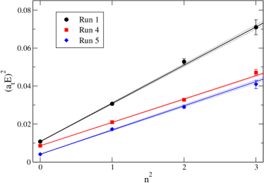
Figure 3: Dispersion relations from runs 1, 4 and 5 on $8^{3}\times 80$ lattices using all-to-all propagators. The solid line is a fit to the four points and the dotted lines are the 68% confidence levels. The quality of all three fits is very good with $\chi^{2}/N_{d.f.}=2.0/2,1.9/2,2.0/2$ for runs 1,4 and 5 respectively.

IV.3 Plane fits

Table 4 shows the output anisotropies determined on the $8^{3}\times 48$ and $8^{3}\times 80$ lattices for the five simulation points.

	$8^{3}\times 48$		$8^{3}\times 80$
Run	$c_{g}$	$\xi_{q}$	$c_{g}$	$\xi_{q}$
1	0.991(3)	4.98(6)	0.972(7)	5.54(6)
2	0.986(3)	6.27(4)
3	1.001(3)	5.18(6)
4	0.985(5)	6.47(5)	0.945(8)	7.08(5)
5	0.995(3)	5.80(5)	0.991(7)	6.95(8)

Table 4: Table of measured output anisotropies at each of the run points. The errors are statistical only.

As a check on the stability of our tuning procedure, we have repeated the calculation using different values of $R$ and $T$ in the determination of the gluon anisotropy. The results are shown in Fig. 4. The plot shows that the anisotropies are insensitive to a change in $R$ but that increasing the value of $T$ from two to three leads to large statistical uncertainty, particularly in the gluon anistropy. For these reasons we choose $R=3$ and $T=2$ for our analysis.

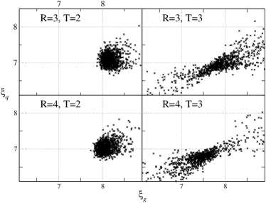
Figure 4: Tuned values of input parameters $(\xi_{g}^{0},\xi_{q}^{0})$ determined from the plane fit procedure on the $8^{3}\times 80$ lattice. The plots show the results for different values of $R$ and $T$ used to determine the gluon anisotropy. Each point corresponds to one bootstrap sample.

IV.4 Simulation with tuned parameters

Applying the plane fit procedure of Sec. IV.3 to a subset of configurations of Runs 1, 4 and 5 we obtained preliminary, tuned parameters $\xi^{0}_{g}=8.06\raisebox{-1.72218pt}{$\stackrel{{\scriptstyle\scriptstyle+7}}{{\scriptstyle-7}}$},\xi^{0}_{q}=7.52\raisebox{-1.72218pt}{$\stackrel{{\scriptstyle\scriptstyle+21}}{{\scriptstyle-15}}$}$. 250 configurations were generated with these parameters, and $c_{g}$ and $\xi_{q}$ determined using the same values for $R$, $T$ and fit ranges as in Sections IV.1 and IV.2. We find $c_{g}=0.983(6),\xi_{q}=6.21(9)$. We see that both quark and gluon anisotropies are within 3% of the target value of 6. Although the anisotropies are not equal within statistical errors, we note that there are still systematic uncertainties at the percent level, in particular for $\xi_{g}$, as shown in Table 2. For example, if we choose $R=3,T=3$ we find $c_{g}=1.01(2)$.

We repeated the plane fit procedure including the new information from Run 6. Figure 5 shows the resulting scatterplot determined on the $8^{3}\times 80$ lattice from runs 1, 4, 5 and 6. The intersection points shift in a direction to move $c_{g}$ and $\xi_{q}$ even closer to the target anisotropy.

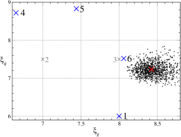
Figure 5: As in Fig 4. The figure shows the results from a plane fit using parameters from runs 1, 4, 5 and 6 (marked with an $\times$). The big red (gray) cross at $(\xi^{0}_{g},\xi^{0}_{q})=(8.42,7.43)$ indicates the result of the best fit.

In order to get a rough idea of the physical scales of these lattices, we compute the pion mass, the rho mass and the string tension. We find $a_{t}m_{\pi}=0.066(1)$ and $a_{t}m_{\rho}=0.120(5)$, which gives $m_{\pi}/m_{\rho}=0.54$, while a crude measurement (shown in Fig. 6) of the string tension gives $a_{s}=0.18$fm.

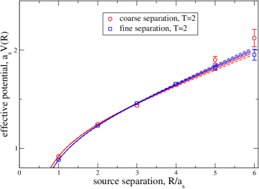
Figure 6: The potential between fundamental static color sources for run 6, measured from static propagation in a coarse direction. Lines show fits to the Cornell potential, and are used in a crude determination of the lattice spacing.

A more precise determination of the lattice spacing will be obtained from the 1P–1S splitting in charmonium Juge:2005nr .

V Conclusions

We have performed a first simulation of 2-flavour QCD with improved Wilson fermions on anisotropic lattices, with both quark and gluon anisotropies tuned to $\xi=6$ . The tuning was based on a linear Ansatz for the dependence of renormalised anisotropies on bare anisotropy parameters in a region of parameter space. The results from the final run demonstrate that the tuning procedure, described in Sec. III, works satisfactorily.

The final, tuned point was found to lie marginally outside the triangle used for the plane fit procedure, so the end result was based on an extrapolation rather than an interpolation. This increases both the statistical and systematic uncertainties of the determination. To avoid this problem, it is important to choose a large enough triangle to start with, so that successive parameter determinations are always based on interpolations.

We also found that the original ($8^{3}\times 48$) lattices used were too short in the time direction to allow a reliable determination of ground state energies, which were found to be systematically high, in particular for higher momenta. This led in turn to systematically high values for $\xi_{q}$. The adoption of lattices with longer time extent was a crucial step in the procedure. As Table 3 shows, the optimal fit ranges were generally found to be beyond the range of the shorter lattice.

We were able to determine the tuned parameters $(\xi^{0}_{g},\xi^{0}_{g})$ with a statistical uncertainty of 1% and 3% respectively from our ensembles of 250 configurations. In addition, there are three main sources of systematic uncertainties:

1. The $R$ and $T$ values used in the determination of the sideways potential, and the fit ranges used in the determination of the pseudoscalar dispersion relation. Since the fit ranges are chosen to give stable ground state energies, we can safely assume that the latter is a small effect. The effect of varying $R$ is also small, as shown in Fig. 4. There may be a systematic error arising from the choice of $T$, but this is obscured by the larger statistical uncertainties in the $T=3$ data, particularly in the $\xi^{0}_{g}$ direction.

2. Lattice sizes. The pion dispersion relation is unlikely to be strongly affected by the finite lattice volume, but the static quark potential may contain finite volume errors which affect our results. We will be performing simulations at the tuned point on larger volumes, which will show whether this is a significant issue.

3. Nonlinearities in the dependence of $(\xi_{g},\xi_{q})$ on $(\xi^{0}_{g},\xi^{0}_{q})$. Our final fit to four points shows no evidence of any significant nonlinearity. If this were found to be a serious issue in any future simulation, a two-step procedure may be adopted where a smaller triangle centred on the preliminary tuned point is used in the second step.

We have yet to verify that we get the same quark anisotropy from other hadronic probes, for example the vector meson. Differences in the anisotropies can arise from lattice artefacts and can thus be considered part of the finite lattice spacing errors.

These lattices will in the future be employed for a wide range of physics investigations, including charm physics and heavy exotics Juge:2005nr , spectral functions at high temperature Morrin:2005zq , static–light mesons and baryons Foley:2005af , strong decays and flavour singlets including glueballs. These studies will be carried out on larger lattice volumes. Simulations on finer lattices will necessitate a new nonperturbative tuning process like the one performed here; this will be desirable in the longer term.

- (1) F. Karsch, Nucl. Phys. B205, 285 (1982).
- (2) CP-PACS, T. Manke et al., Phys. Rev. Lett. 82, 4396 (1999), [hep-lat/9812017].
- (3) C. J. Morningstar and M. J. Peardon, Phys. Rev. D60, 034509 (1999), [hep-lat/9901004].
- (4) M. Asakawa and T. Hatsuda, Phys. Rev. Lett. 92, 012001 (2004), [hep-lat/0308034].
- (5) S. Hashimoto and M. Okamoto, Phys. Rev. D67, 114503 (2003), [hep-lat/0302012].
- (6) N. Ishii, T. Doi, Y. Nemoto, M. Oka and H. Suganuma, Phys. Rev. D72, 074503 (2005), [hep-lat/0506022].
- (7) TrinLat, J. Foley, A. Ó Cais, M. Peardon and S. M. Ryan, Phys. Rev. D73, 014514 (2006), [hep-lat/0405030].
- (8) M. G. Alford, I. T. Drummond, R. R. Horgan, H. Shanahan and M. J. Peardon, Phys. Rev. D63, 074501 (2001), [hep-lat/0003019].
- (9) T. R. Klassen, Nucl. Phys. B533, 557 (1998), [hep-lat/9803010].
- (10) C. Morningstar and M. J. Peardon, Nucl. Phys. Proc. Suppl. 83, 887 (2000), [hep-lat/9911003].
- (11) C. Morningstar and M. J. Peardon, Phys. Rev. D69, 054501 (2004), [hep-lat/0311018].
- (12) R. Morrin, M. Peardon and S. M. Ryan, PoS LAT2005, 236 (2005), [hep-lat/0510016].
- (13) M. J. Peardon, Nucl. Phys. Proc. Suppl. 109A, 212 (2002).
- (14) S. Duane, A. D. Kennedy, B. J. Pendleton and D. Roweth, Phys. Lett. B195, 216 (1987).
- (15) J. Foley et al., Comp. Phys. Commun. 172, 145 (2005), [hep-lat/0505023].
- (16) K. J. Juge, A. Ó Cais, M. B. Oktay, M. J. Peardon and S. M. Ryan, PoS LAT2005, 029 (2005), [hep-lat/0510060].
- (17) R. Morrin et al., PoS LAT2005, 176 (2005), [hep-lat/0509115].
- (18) J. Foley et al., PoS LAT2005, 216 (2005), [hep-lat/0511005].
- (19) L. Levkova, T. Manke and R. Mawhinney, Phys. Rev. D73, 074504 (2006), [hep-lat/0603031].