Analysis of systematic errors in the calculation of renormalization constants of the topological susceptibility on the lattice

Abstract

A Ginsparg–Wilson based calibration of the topological charge is used to calculate the renormalization constants which appear in the field–theoretical determination of the topological susceptibility on the lattice. A systematic comparison is made with calculations based on cooling. The two methods agree within present statistical errors (3%–4%). We also discuss the independence of the multiplicative renormalization constant $Z$ from the background topological charge used to determine it.

I Introduction

Topology in QCD plays a relevant rôle in understanding several low energy properties of the theory. One of the quantities that have a direct interest in phenomenology is the topological susceptibility $\chi$ which is defined as the correlator at zero momentum of two topological charge density operators $Q(x)$. In particular the value of $\chi$ in the pure gauge theory is interpreted in terms of the mass of the singlet pseudoscalar meson witten ; veneziano .

The lattice is an excellent tool to calculate such dimensionful observables and specifically the lattice determination of $\chi$ in the pure gauge theory is in good agreement with phenomenological expectations alles ; lucini ; giusti .

The calculation of $\chi$ or any other topology–related quantity on the lattice requires a regularization $Q_{L}(x)$ of the topological charge density operator. The formal naïve continuum limit must satisfy $Q_{L}(x){\buildrel a\rightarrow 0\over{\longrightarrow}}a^{4}Q(x)$, ($a$ is the lattice spacing).

However in general $Q_{L}(x)$ does not meet the continuum Ward identities crewther . Consequently the lattice definition of the topological susceptibility $\chi_{L}\equiv\langle Q_{L}^{2}\rangle/V$ ($V$ is the lattice volume and $Q_{L}\equiv\sum_{x}Q_{L}(x)$) need not coincide with the physical continuum expression $\chi$. The two quantities are related by nupha329 ; haris

$$\chi_{L}=Z^{2}a^{4}\chi+M\,,$$ (1)

where $Z$ and $M$ are renormalization constants which for evident reasons are called multiplicative and additive respectively. In order to extract $\chi$ from the lattice data of $\chi_{L}$ one must know the values of $Z$ and $M$.

Let us outline the origin of the two renormalization constants. Any matrix element which contains $n$ insertions of the topological charge operator can be calculated either in the continuum (with an adequate regularization) or on the lattice. In general the two calculations match only after the inclusion of a multiplicative renormalization constant $Z$ haris ; vicari for each insertion of $Q(x)$. In a formal writing, $Q_{L}(x)=Za^{4}Q(x)$ where $Z$ is a finite renormalization constant. In the theory with fermions the topological charge mixes with other operators related to the axial anomaly espriu . This mixing induces a correction to the above described multiplicative renormalization and consequently also to Eq.(1). Such a correction is however rather small alles5 and it is usually neglected consistently with the large statistical errors from a typical numerical simulation.

If $n\geq 2$ the above matrix element includes further divergences which are the origin of the additive term $M$. In fact the expression for $\chi$ contains the product of two topological charges at the same spacetime point. The operator expansion of this product at short distances contains mixings with operators that share the quantum numbers of $\chi$. On the other hand it is known that the correlation function of two topological charge operators at nonzero distance is negative osterwalder ; seiler , $\langle Q(x)Q(0)\rangle<0$ for $x\not=0$. This inequality also holds on the lattice for any definition of $Q_{L}(x)$ menotti ; kirchner ; horvath ; ilgenfritz . Since $\chi$ is a positive quantity, part of the contact terms must be included in the physical definition of $\chi$. The rest of the terms, if any, must be subtracted and they are $M$.

A prescription is necessary to calculate $M$. Due to the expression $\chi={\rm d}^{2}\ln Z(\theta)/{\rm d}\theta^{2}|_{\theta=0}$ where $Z(\theta)$ is the partition function of the gauge theory with a theta term, we know that $\chi$ vanishes within the zero topological charge sector. We then adopt the following definition for $M$: it is the value of $\chi_{L}$ in the sector of zero topological charge, $M\equiv\chi_{L}|_{q=0}$ where $q$ is the value of the total topological charge of a configuration (as determined by cooling or other means, see later).

A nonperturbative method to calculate $Z$ and $M$ has been developed in Refs. vicari2 ; gunduc . The method will be described in Section 2. It has been used in several calculations of topological properties in QCD and other theories. Various tests and studies of efficiency have also been worked out in the past. In Section 3 we will present the main contribution of the paper: a study of systematic errors that may affect the calculation of the renormalization constants and a comparison of results when they are obtained by using different methods for calibrating the background topological sector. Some conclusive comments are given in Section 4.

II The nonperturbative calculation of $M$ and $Z$

In Refs. vicari2 ; gunduc a technique, called “heating method”, to calculate the renormalization constants in Eq.(1) was put forward. The idea behind the heating method is that the UV fluctuations in $Q_{L}(x)$, which are the ultimate cause for renormalizations, are effectively decoupled from the background topological signal so that, starting from a classical configuration of fixed topological content, it is possible, by applying a few updating (heating) steps at the corresponding value of the lattice bare coupling constant $\beta$, to thermalize the UV fluctuations without altering the background topological content. This result is favoured by the fact that topological modes have very large autocorrelation times, as compared to other non–topological observables (this autocorrelation time is particularly long in the case of full QCD vicari3 ; lippert and also in the case of a large number of colours ddpp ).

One can thus create samples of configurations within a given topological sector $q$ with the UV fluctuations thermalized. If $q\not=0$ then the measurement of $Q_{L}$ on such a sample leads to the lattice value of the background topological charge $q_{L}$. As described above haris ; vicari , this result must be renormalized to match the continuum value $q$,

$$q_{L}\equiv\langle Q_{L}\rangle|_{q}=Zq\,,$$ (2)

where the subscript $|_{q}$ indicates that the thermalization is achieved within the sector of charge $q$. Therefore, knowing $q$ from the classical configuration and determining $q_{L}$ from the measurement of $Q_{L}$ on the sample, $Z$ can be extracted.

If $q=0$ then measuring $Q_{L}^{2}/V$ on the sample leads to the value $\chi_{L}|_{q=0}$ which is precisely $M$, as indicated above.

$M$ can also be calculated on samples with nonvanishing topological background $q$. Following Eq.(1) and Eq.(2) the additive constant is extracted in this case by using the relation

$$M=\frac{1}{V}\left(\langle Q_{L}^{2}\rangle|_{q}-\left(\langle Q_{L}\rangle|_{q}\right)^{2}\right)$$ (3)

and leads to the same results vicari2 ; delia .

A sample of configurations belonging to the sector of total topological charge $q$ is obtained in the following way. One starts from a classical configuration with topological charge $q$. It can be easily obtained either by using cooled configurations where the energy and the topological charge correspond to the presence of one instanton (if $q=1$) or by setting all gauge links to unity (if $q=0$). Then a few updating steps are applied and the proper operator (either $Q_{L}$ or $Q_{L}^{2}/V$) is measured at each step. Moreover at each step the background topological charge is checked by cooling teper1 in order to verify that the configuration still lies in the sector of charge $q$ papafarchioni . When the result of the measurement stabilizes (data display a plateau), while $q$ stays fixed, we consider that the UV fluctuations are thermalized and $\langle Q_{L}\rangle|_{q=1}$ and $\langle Q_{L}^{2}/V\rangle|_{q=0}$ yield $Z$ and $M$ respectively.

When the cooling applied to a configuration reveals that its background topological charge is no longer equal to $q$ then the configuration is discarded from the sample. However it might also happen the following event: a possible new instanton or anti–instanton created by the various updating steps might evade the cooling probe because the very cooling procedure could destroy it (this may happen especially when the instanton spans a few lattice spacings). In this case we would include in the sample a configuration which actually does not belong to the sector of topological charge $q$. Such an event would obviously distort the measurement of any of the above topological operators. For example, it yields an overestimation of $\langle Q_{L}^{2}\rangle|_{q=0}$ because any added instanton or anti–instanton only increments the value of the square. On the other hand since the theory predilects the sector of vanishing topological charge, the updating steps during the calculation of $Z$ tend to bring the configuration to that sector either by destroying the original instanton or by creating from scratch an anti–instanton. As a consequence the value of $\langle Q_{L}\rangle|_{q=1}$ becomes underestimated because on average the expectation value of $Q_{L}$ in the sector $q=0$ is less than in the sector with $q=1$.

In the past we have always been aware of that potential problem and in this paper we present a study where the background topological sector is calibrated by another method in order to compare the results and detect any difference in the form of a systematic error. The new method is the counting of zero modes by using Ginsparg–Wilson based operators ginspargwilson and it will be described in the next Section.

III A study of systematic errors

Following the lines described in the above Section, we have calculated the values of the renormalization constants in Eq.(1) for the 1–smeared topological charge operator defined as viejo

$$Q_{L}(x)=-\frac{1}{2^{9}\pi^{2}}\sum_{\mu\nu\rho\sigma=\pm 1}^{\pm 4}\widetilde{\epsilon}_{\mu\nu\rho\sigma}{\rm Tr}\left\{\Pi_{\mu\nu}(x)\Pi_{\rho\sigma}(x)\right\}\,,$$ (4)

where all link matrices have been substituted by 1–smeared links cristo (the smearing parameter was $c=0.90$). The corresponding renormalization constants will be called $M^{(1)}$ and $Z^{(1)}$ to denote the level of smearing. In the above expression $\Pi_{\mu\nu}(x)$ is the plaquette in the $\mu-\nu$ plane with the four corners at $x$, $x+\widehat{\mu}$, $x+\widehat{\mu}+\widehat{\nu}$, $x+\widehat{\nu}$ (counter–clockwise path). Links pointing to negative directions mean $U_{-\mu}(x)\equiv U_{\mu}^{\dagger}(x-\widehat{\mu})$. The generalized completely antisymmetric tensor is defined by $\widetilde{\epsilon}_{1234}=1$ and $\widetilde{\epsilon}_{(-\mu)\nu\rho\sigma}=-\widetilde{\epsilon}_{\mu\nu\rho\sigma}$. The calculation was performed for the Yang–Mills theory with SU(3) gauge group and Wilson action waction . The lattice size was $12^{4}$ and the bare coupling $\beta=6$.

The practical procedure was the following: starting from a classical configuration with the adequate topological background content ($q=0$ for $M^{(1)}$ or $q=1$ for $Z^{(1)}$), 80 heat–bath (HB) steps were applied, each step consisting of three Cabibbo–Marinari cabibbom hits, one for each SU(2) subgroup and Kennedy–Pendleton algorithm kennedyp for refreshing the dynamical variables. The operator ($(Q_{L})^{2}/V$ for $M^{(1)}$ or $Q_{L}$ for $Z^{(1)}$) was measured every 4 steps. This set of 20 measurements is called “trajectory”. A test of the topological sector was accomplished after each measurement on a separate copy of the configuration. We accepted only those measurements that were thermalized within the corresponding topological sector. This condition means that the data must have stabilized to a plateau and that the test must have revealed that the configuration lay within the correct topological sector. The average over all accepted measurements yielded $M^{(1)}$ or $Z^{(1)}$.

The test was performed by two different methods: either by a traditional cooling teper1 or by counting fermionic zero modes (CFZM). This last method consists in calculating the net number of zero modes, $n_{+}-n_{-}$ by enumerating the level crossings in the spectrum of the Wilson–Dirac operator $D_{W}-am$ as the fermion mass $m$ is varied naraya ; neuberg ; edwards . This method was utilized in Refs. edwards ; deldebbio to calculate the topological charge.

The main advantage of the CFZM method against cooling is that the first one does not need to modify the configuration to which it is applied, hence the topological content is never altered during the test. On the contrary its main disadvantage is that its implementation is heavily time–consuming.

Let us discuss in more detail the CFZM method. We can stop counting crossings at any mass $am=am_{\rm stop}$ inside the allowed interval $am<2$. Thus, in general the measurement of the topological charge will depend on $am_{\rm stop}$ because there can be level crossings all along the interval of masses where the gap is closed. This makes the zero mode counting method to look ambiguous. However in Ref. edwards it is shown that such a dependence is rather mild for $\beta\approx 6$ as long as $am_{\rm stop}>1.5$. In the present work we have sought crossings up to three different values for the stopping mass: $1.0$, $1.5$ and $2.0$. In particular the last (and largest possible) value looks particularly interesting because instantons representing crossings close to $am=2.0$ span a size of a few lattice spacings edwards , i.e.: they are the instantons that most likely could evade the cooling test.

The search for crossings was realized by following the same procedure of Ref. deldebbio . An accelerated conjugate gradient algorithm bunk was employed to extract the lowest eigenvalues of the Wilson–Dirac operator.

The topological charge after the cooling test was required to be equal to 1 or 0 within a tolerance of $\delta$. We usually chose $\delta=0.3$ although tests with other values were performed (see later) proving that the results are very robust against variability of $\delta$.

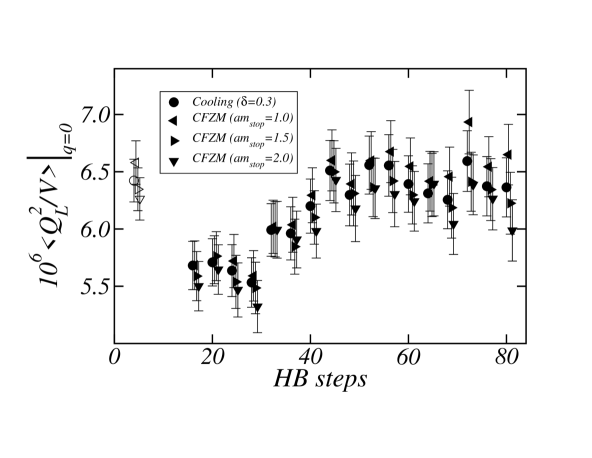
Figure 1: $\langle Q_{L}^{2}/V\rangle|_{q=0}$ as a function of the HB step for the four calibration tests described in the text. The results for $M^{(1)}$ have been placed on the left side and are represented by white symbols. Data corresponding to different calibration methods have been shifted with respect to each other in order to render the Figure clearer.

III.1 Systematic errors on $M^{(1)}$

The results for $M^{(1)}$ are shown in Fig. 1. We have calculated 1380 trajectories of 80 HB steps and measured the operator $Q_{L}^{2}/V$ every 4 steps after checking that the background charge was zero. For each measurement, in the Figure we show the average over all the results. Actually we show the data after the 16$th$ step because measurements after too few HB steps are irrelevant as the configuration is surely not yet thermalized. A plateau seems to set in after approximately 40 steps which indicates that thermalization has been achieved. Then the value of $M^{(1)}$ can be extracted by averaging over the data after the 40$th$ step.

The error bar was calculated in the following manner: each trajectory was treated as a single data by averaging all accepted (i.e.: all thermalized and correctly calibrated) points in it. Since separate trajectories are prepared by independent Monte Carlo runs, this procedure guarantees the absence of autocorrelations. Then the average and the error are easily obtained from this set of 1380 data. Furthermore, due to the fact that different trajectories can contain a variable number of accepted points, each trajectory must be weighted by a factor proportional to the number of accepted points in it.

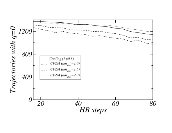
Figure 2: Counting of trajectories that still lie in the $q=0$ topological sector as the number of HB steps increases for the four calibration methods.

If the number of accepted points in the trajectory $t$ is $n_{t}$ and if $T_{t}$ is the average over all accepted measurements $m$ in this trajectory,

$$T_{t}=\frac{1}{n_{t}}\sum_{m\in t}\left(\frac{Q^{2}_{L}}{V}\right)_{m}\Bigg{|}_{\buildrel q=0\over{\rm thermalized}}\;,$$ (5)

then

$$M^{(1)}=\frac{\sum_{t}T_{t}n_{t}}{\sum_{t}n_{t}}\;.$$ (6)

Fig. 1 displays the results for all four methods of calibration, cooling with $\delta=0.3$ and CFZM with three different values for the stopping mass. The four white symbols on the left side of the Figure are the corresponding results for $M^{(1)}$. They become smaller as the value of $am_{\rm stop}$ is incremented. This effect is possibly an indication of a systematic error which however has little effect in the calculation since all results look compatible with each other within errors. It must be stressed that the statistical errors, represented by the error bars in the Figure, amount to about 3% which is rather small.

In Fig. 2 we show, for each measurement, the number of trajectories for which the calibration test gave an acceptable result, $q=0$. The plot is shown for all measurements, thermalized or not, from the 20$th$ HB step onward. The maximum possible number is obviously 1380 and it falls off as the amount of HB steps is increased. The decrease is steeper for the CFZM with larger stopping mass. In the latest step and for the CFZM with $am_{\rm stop}=2$ about 30% of all trajectories have varied the topological sector, while for the cooling method the analogous percentage is about 17%. Such a difference still allows to obtain results for $M^{(1)}$ that are compatible within (small) errors, as shown by the white symbols in Fig. 1.

The values of $M^{(1)}$ obtained by using cooling with varying $\delta$ are indistinguishable from each other (white circle in Fig. 1) for $\delta$ ranging from 0.1 to 0.5. In Fig. 3 three tolerance parameters for cooling are compared indicating that the three tests are almost completely equivalent. Again the maximum possible number of trajectories with the right background topological charge is 1380 and it diminishes as the amount of HB steps is increased. This number became 1136 for $\delta=0.1$ at the latest step.

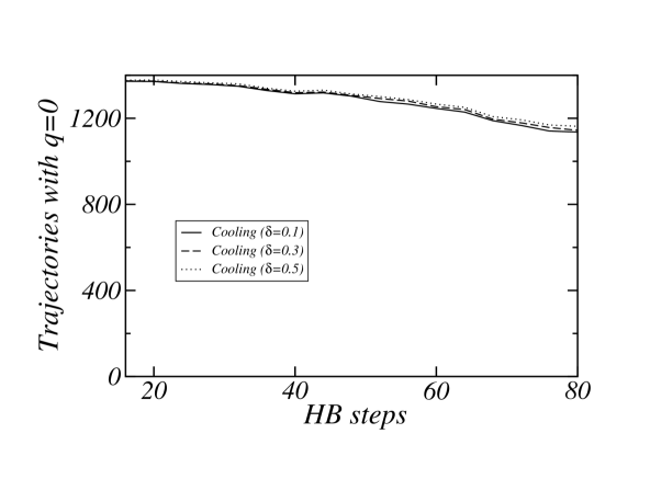
Figure 3: Counting of trajectories that still lie in the $q=0$ topological sector as the number of HB steps increases for the cooling method with three different values of $\delta$.

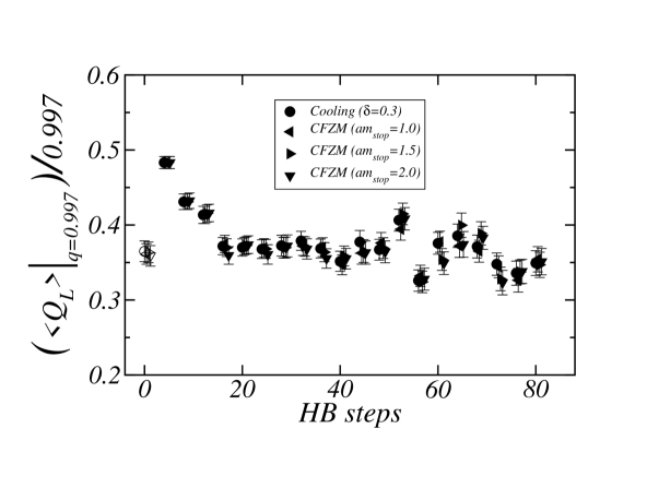
Figure 4: Averages of $\left(\langle Q_{L}\rangle|_{q}\right)/q$ as a function of the HB step for the four calibration methods. An instanton with charge $q=0.997$ was used. The values of $Z^{(1)}$ correspond to the height of the plateau and they are indicated on the left hand side of the plot with white symbols. Data corresponding to different calibration methods have been slightly shifted for clarity.

III.2 Systematic errors on $Z^{(1)}$

Fig. 4 displays the analogous study of Fig. 1 for the calculation of $Z^{(1)}$. An instanton with topological charge (as measured with $Q_{L}$ after cooling) $q=0.997$ was employed. The procedure for the calculation of $Z^{(1)}$ resembles very much that of the $M^{(1)}$. We prepared 840 independent trajectories and again the calibration was performed by four different tests, as indicated in Fig. 4. The average per trajectory is $T_{t}$,

$$T_{t}=\frac{1}{n_{t}}\sum_{m\in t}\left(Q_{L}\right)_{m}\Bigg{|}_{\buildrel q=0.997\over{\rm thermalized}}\;,$$ (7)

and the result for $Z^{(1)}$ is

$$Z^{(1)}=\frac{1}{0.997}\,\frac{\sum_{t}T_{t}n_{t}}{\sum_{t}n_{t}}\;.$$ (8)

A plateau sets in at about the 20$th$ HB step. Figures similar to Fig. 2 and 3 are obtained with analogous conclusions. Again the coincident results (white symbols in Fig. 4) indicate that all calibration methods are equivalent in such a way that any systematic error implicit in our method has negligible consequences within our precision (statistical errors in Fig. 4 are about 4%).

Table 1: $Z^{(1)}$ for the 1–smeared operator as a function of $\beta$ for several values of the background topological charge $q$. Instantons with charge $q\approx-1$, $\approx+1$ and $\approx+2$ are used on a lattice volume $16^{4}$.

$\;\beta\;$	$\;q=+0.990\;$	$\;q=-0.988\;$	$\;q=+0.955\;$	$\;q=-0.902\;$	$\;q=+1.941\;$
6.00	0.373(20)	0.383(15)	0.370(20)	0.365(20)	0.390(12)
6.20	0.432(6)	–	–	–	0.441(5)
6.50	0.503(11)	–	–	–	0.506(5)

Table 2: $Z^{(2)}$ for the 2–smeared operator as a function of $\beta$ for several values of the background topological charge $q$. Instantons with charge $q\approx-1$, $\approx+1$ and $\approx+2$ are used on a lattice volume $16^{4}$.

$\;\beta\;$	$\;q=+0.990\;$	$\;q=-0.988\;$	$\;q=+0.955\;$	$\;q=-0.902\;$	$\;q=+1.941\;$
6.00	0.500(12)	0.503(13)	0.495(15)	0.487(20)	0.499(16)
6.20	0.560(6)	–	–	–	0.569(4)
6.50	0.620(10)	–	–	–	0.631(3)

It is well–known that the total topological charge of isolated classical instantons in general is not equal to integer numbers when it is calculated with the operator of Eq.(4). The difference between the value of the charge and the closest corresponding integer ($|1-q|$ in our case) becomes negligible when the inequalities $a\ll\rho\ll La$ hold ($\rho$ being the instanton size and $L$ the lattice size). A simple calculation shows that the value of $q$ for a discretized instanton in a volume $L^{4}$ is given by

$$q\approx 1-3\left(\frac{\rho}{La}\right)^{4}\;,$$ (9)

while the discretization error is totally negligible if $a\lesssim\rho/3$. The ratio $a/\rho$ can be estimated by looking at the action density distribution. We expect that the infrared effect described in Eq.(9) cancels out if we divide the charge after heating by the initial value $q$ as indicated in Eq.(2). This fact was carefully checked in becca for the 2D $O(3)$ nonlinear sigma model. It was also used in Eq.(8) although in that case and within our errors, the $q=0.997$ in the denominator is indistinguishable from 1. In the present study we have verified it for our gauge theory: in Table 1 and 2 the multiplicative constant is calculated at several values of the gauge bare coupling $\beta$ on a $16^{4}$ volume starting from various initial instantons for the 1– and 2–smeared operators (they are constructed as in Eq.(4) after substituting all links with 1– and 2–smeared links respectively cristo ). A number of trajectories ranging from 200 to 500 were used. Notice that within errors the values for $Z^{(1)}$ and $Z^{(2)}$ display a dependence on $\beta$ but not on $q$ as long as data are divided by the initial value $q$, as described above following Eq.(2). If instead data were divided by the integer closest to $q$ then the results for $Z^{(i)}$, $(i=1,2)$ would display a fake dependence also on $q$. This fact is seen in Fig. 5 where the values of $Z^{(2)}$ are displayed as a function of $q$ after dividing by $q$ (squares) or by the closest integer to $q$ (triangles): only the squares show constancy with respect to $q$. Within our statistical errors the systematic error is negligible down to $q\approx 0.9$. Possibly if the statistics were increased this limit could grow. In any case to calculate $Z$ it is better to make use of instantons with $q$ as close as possible to an integer.

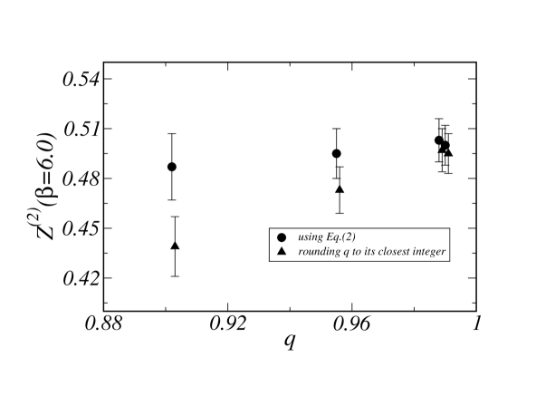
Figure 5: $Z^{(2)}(\beta=6.0)$ as obtained by using four several initial classical instantons (with $|q|=$0.902, 0.955, 0.988 and 0.0990). Squares stand for the results obtained by applying Eq.(2) and triangles by applying the same equation after rounding the value of $q$ to its closest integer.

IV Conclusions

We have studied two possible sources of systematic errors in the nonperturbative determination of the renormalization constants for the evaluation of the topological susceptibility on the lattice, $Z$ and $M$ (see Eq.(1)):

• i) The cooling test of the background topological charge along the heating process could yield a wrong information since the cooling procedure could delete the unwanted instanton or anti–instanton created by the heating steps. An independent check of the cooling test has been performed by applying calibration methods based on the counting of fermionic zero modes. No sizeable systematic effects have been observed within our (rather small) statistical errors (3% for $M$ and 4% for $Z$).

• ii) In the calculation of $Z$ for the operator $Q_{L}$ of Eq.(4) the simulation must be started from a configuration with a topological charge $q$ different from zero. In the infinite volume limit $q$ takes on integer values, however on the lattice, the determination of $q$ by using the operator in Eq.(4), leads to results which in general are close to but not strictly equal to integers. We have argued that this is a potential source of error that can affect the calculation of $Z$. However it can be kept under control if one uses Eq.(2) to extract $Z$ with $q$ not rounded to its closest integer.

In conclusion one can safely use the field–theoretical method to study topology on the lattice since any possible systematic error of the method is well under control. Moreover the method is much less demanding in computer time than the Ginsparg–Wilson based method.

The APEmille facility in Pisa was used for part of the runs.

References

- (1) E. Witten, Nucl. Phys. B156 (1979) 269.
- (2) G. Veneziano, Nucl. Phys. B159 (1979) 213.
- (3) B. Allés, M. D’Elia, A. Di Giacomo, Phys. Rev. D71 (2005) 034503.
- (4) B. Lucini, M. Teper, U. Wenger, Nucl. Phys. B715 (2005) 461.
- (5) L. Del Debbio, L. Giusti, C. Pica, Phys. Rev. Lett. 94 (2005) 032003.
- (6) R. J. Crewther, Riv. Nuovo Cimento 2 (1979) 8.
- (7) M. Campostrini, A. Di Giacomo, H. Panagopoulos, E. Vicari, Nucl. Phys. B329 (1990) 683.
- (8) M. Campostrini, A. Di Giacomo, H. Panagopoulos, Phys. Lett. B212 (1988) 206.
- (9) B. Allés, E. Vicari, Phys. Lett. B268 (1991) 241.
- (10) D. Espriu, R. Tarrach, Z. Phys. C16 (1982) 77.
- (11) B. Allés, A. Di Giacomo, H. Panagopoulos, E. Vicari, Phys. Lett. B350 (1995) 70.
- (12) K. Osterwalder in “Constructive Field Theory”, Lecture Notes in Physics, no 25, 1973, edited by G. Velo, A. S. Wightman.
- (13) E. Seiler, I. O. Stamatescu, preprint MPI-PAE/PTh 10/87 (1987) unpublished.
- (14) P. Menotti, A. Pelissetto, Nucl. Phys. B (Proc. Suppl.) 4 (1988) 644.
- (15) B. Allés, M. D’Elia, A. Di Giacomo, R. Kirchner, Phys. Rev. D58 (1998) 114506.
- (16) I. Horváth et al., Phys. Lett. B617 (2005) 49.
- (17) E.–M. Ilgenfritz, K. Koller, Y. Koma, G. Schierholz, T. Streuer, V. Weinberg, hep–lat/0512005.
- (18) A. Di Giacomo, E. Vicari, Phys. Lett. B275 (1992) 429.
- (19) B. Allés, M. Campostrini, A. Di Giacomo, Y. Gündüç, E. Vicari, Phys. Rev. D48 (1993) 2284.
- (20) B. Allés, G. Boyd, M. D’Elia, A. Di Giacomo, E. Vicari, Phys. Lett. B389 (1996) 107.
- (21) B. Allés et al., Phys. Rev. D58 (1998) 071503.
- (22) L. Del Debbio, H. Panagopoulos, P. Rossi, E. Vicari, Phys. Rev. D65 (2002) 021501.
- (23) M. D’Elia, Nucl. Phys. B661 (2003) 139.
- (24) A. A. Belavin, A. M. Polyakov, A. S. Schwartz, Yu. S. Tyupkin, Phys. Lett. B59 (1975) 85.
- (25) I. A. Fox, M. L. Laursen, G. Schierholz, J. P. Gilchrist, M. Göckeler, Phys. Lett. B158 (1985) 332.
- (26) M. Teper, Phys. Lett. B171 (1986) 81; Phys. Lett. B171 (1986) 86.
- (27) B. Allés, L. Cosmai, M. D’Elia, A. Papa, Phys. Rev. D62 (2000) 094507.
- (28) F. Farchioni, A. Papa, Nucl. Phys. B431 (1994) 686.
- (29) P. H. Ginsparg, K. G. Wilson, Phys. Rev. D25 (1982) 2649.
- (30) P. Di Vecchia, K. Fabricius, G. C. Rossi, G. Veneziano, Nucl. Phys. B192 (1981) 392; Phys. Lett. B108 (1982) 323.
- (31) C. Christou, A. Di Giacomo, H. Panagopoulos, E. Vicari, Phys. Rev. D53 (1996) 2619.
- (32) K. G. Wilson, Phys. Rev. D10 (1974) 2445.
- (33) N. Cabibbo, E. Marinari, Phys. Lett. B119 (1982) 387.
- (34) A. D. Kennedy, B. J. Pendleton, Phys. Lett. B156 (1985) 393.
- (35) R. Narayanan, H. Neuberger, Nucl. Phys. B443 (1995) 305.
- (36) H. Neuberger, Phys. Rev. D61 (2000) 085015.
- (37) R. G. Edwards, U. M. Heller, R. Narayanan, Nucl. Phys. B535 (1998) 403.
- (38) L. Del Debbio, C. Pica, JHEP 02 (2004) 003.
- (39) B. Bunk, K. Jansen, M. Lüscher, H. Simma, “Conjugate gradient algorithm to compute the low–lying eigenvalues of the Dirac operator in lattice QCD”, unpublished report (1994); T. Kalkreuter, H. Simma, Comput. Phys. Comm. 93 (1996) 33.
- (40) B. Allés, M. Beccaria, F. Farchioni, Phys. Rev. D54 (1996) 1044.