Non-perturbative mass spectrum of an extra-dimensional orbifold

Abstract

We analyse non-perturbatively a five-dimensional $SU(2)$ gauge theory compactified on the $S^{1}/\mathbb{Z}_{2}$ orbifold. In particular, we present simulation results for the mass spectrum of the theory, which contains a Higgs and a photon. The Higgs mass is found to be free of divergences without fine-tuning. The photon mass is non-zero, thus providing us with the first lattice evidence for a Higgs mechanism derived from an extra dimension. Data from the static potential are consistent with dimensional reduction at low energies.

I Introduction

An attempt to embed the Standard Model in a more general theory reveals subtleties associated with its Higgs sector such as the fine-tuning problem and, if for example the larger theory includes also gravity, the hierarchy problem. The former is essentially a reflection of the quadratic sensitivity of the Higgs mass to the ultra-violet cut-off and the latter refers to the mystery associated with the smallness of the ratio of the electroweak and Planck scales $M_{\rm EW}/M_{\rm Pl}$. Supersymmetry provides a possible solution to the fine-tuning problem but at the cost of introducing many new couplings and degrees of freedom into the Standard Model. This is of course not necessarily a disaster, especially if low-energy supersymmetry is confirmed at the LHC. Since however the latter is not guaranteed, it is perhaps wise to think of alternative scenarios.

In this Letter, we present results from the investigation of a simple model, which gives a possible explanation of the origin of the Higgs field and at the same time does not suffer from a fine-tuning problem. Since we carry out our analysis in the context of gauge theories, we will not have anything to say about the hierarchy problem. Also, in order to illustrate in the simplest possible way the underlying physics, we would like to postpone technical details to a later work.

The model we will consider is a five-dimensional pure $SU(2)$ gauge theory with its fifth dimension compactified on the $S^{1}/\mathbb{Z}_{2}$ orbifold , and with the $\mathbb{Z}_{2}$ acting as a reflection of the extra-dimensional coordinate. It is possible to embed the $\mathbb{Z}_{2}$ action into the gauge group so that it breaks on the orbifold boundaries to a $U(1)$ subgroup, which results in the appearance of a complex scalar field with the four-dimensional quantum numbers of a Higgs field Antoniadis et al. (2001). At the classical level the scalar is massless. However at 1 loop, a dynamically generated potential is formed and the scalar can in principle further break the gauge group spontaneously by taking a vacuum expectation value. Perturbative studies have revealed that the presence of bulk fermions or scalars is necessary for this mechanism to work Hosotani (1983, 1989); Kubo et al. (2002) but a non-zero Higgs mass is generated anyway, just as one would expect by trivially extending results obtained in finite-temperature field theory Zinn-Justin (2002) or as one can verify by a computation in the Kaluza–Klein framework von Gersdorff et al. (2002a); Cheng et al. (2002). In fact, the Kaluza–Klein expansion, being a gauge in which the states in the Hilbert space are diagonalized with respect to their four-dimensional quantum numbers is the one that best fits the perturbative approach to compactified extra-dimensional field theories. In a non-perturbative approach it seems necessary, though, to keep the entire gauge invariance intact, and thus the Kaluza–Klein construction is less useful.

II Orbifold on the lattice

As an alternative approach to perturbation theory, we use the non-perturbative definition of five-dimensional $SU(N)$ gauge theories compactified on the $S^{1}/\mathbb{Z}_{2}$ orbifold Irges and Knechtli (2005) and analyse the system via lattice simulations . The first signal of interesting non-perturbative physics can be anticipated by looking at the lattice coupling

$$\beta=\frac{2N}{g_{5}^{2}}a,$$ (1)

where $a$ is the lattice spacing (which provides the inverse cut-off $1/\Lambda$) and $g_{5}$ is the five-dimensional gauge coupling, which has mass dimension $-1/2$. The latter can be thought of as an effective coupling at the cut-off scale. Naive dimensional analysis tells us that as $\beta$ decreases with $g_{5}$ fixed, the lattice spacing also decreases and the dimensionless bare coupling $g_{0}=g_{5}\sqrt{1/a}$ blows up. One would therefore expect to find the perturbative regime in the large-$\beta$ region where the lattice spacing is large and the bare coupling small. The compactification scale is $1/R$, with $R$ the radius of $S^{1}$ and a separation from the cut-off scale requires $a/R\ll 1$. Increasing $\beta$ would require an increase also of $R$, which drives the fifth dimension to its decompactification limit; as a result the system degenerates to a theory of massless photons. A general lesson from the above discussion then is that moving towards the perturbative regime is expected to enhance the cut-off effects (appearing as $E/\Lambda$ at low energies $E$ in the sense of an effective action) and decompactify the theory, whereas moving in the opposite direction, i.e. towards small $\beta$, is expected to suppress the cut-off effects and drive the system into a compactified but non-perturbative regime. Eventually a phase transition is reached at a critical value of $\beta$ Creutz (1979); Beard et al. (1998); Knechtli et al. (2005), where the cut-off reaches its maximal value. The viability of perturbative extra-dimensional extensions of the Standard Model then essentially relies on the existence of an overlap between these two regimes and clearly a computational method that can probe both of them, such as the lattice, could provide us with a unique insight.

Gauge theories on the orbifold can be discretized on the lattice Irges and Knechtli (2005); Knechtli et al. (2005). One starts with a gauge theory formulated on a five-dimensional torus with lattice spacing $a$ and periodic boundary conditions in all directions $M=0,1,2,3,5$. The spatial directions ($M=1,2,3$) have length $L$, the time-like direction ($M=0$) has length $T$, and the extra dimension ($M=5$) has length $2\pi R$. The coordinates of the points are labelled by integers $n\equiv\{n_{M}\}$ and the gauge field is the set of link variables $\{U(n,M)\in SU(N)\}$. The latter are related to a gauge potential $A_{M}$ in the Lie algebra of $SU(N)$ by $U(n,M)=\exp\{aA_{M}(n)\}$. Embedding the orbifold action in the gauge field on the lattice amounts to imposing on the links the $\mathbb{Z}_{2}$ projection

$$(1-\Gamma)U(n,M)=0\,,$$ (2)

where $\Gamma={\cal R}{\cal T}_{g}$. Here, ${\cal R}$ is the reflection operator that acts as ${\cal R}\,n=(n_{\mu},-n_{5})\equiv\bar{n}\;(\mu=0,1,2,3)$ on the lattice and as ${\cal R}\,U(n,\mu)=U(\bar{n},\mu)$ and ${\cal R}\,U(n,5)=U^{\dagger}(\bar{n}-{\hat{5}},5)$ on the links. The group conjugation ${\cal T}_{g}$ acts only on the links, as ${\cal T}_{g}U(n,M)=gU(n,M)g^{-1}$, where $g$ is a constant $SU(N)$ matrix with the property that $g^{2}$ is an element of the centre of $SU(N)$. For $SU(2)$ we will take $g=-i\sigma^{3}$. Only gauge transformations $\{\Omega(n)\}$ satisfying $(1-\Gamma)\Omega=0$ are consistent with Eq. (2). This means that at the orbifold fixed points, for which $n_{5}=0$ or $n_{5}=\pi R/a=N_{5}$, the gauge group is broken to the subgroup that commutes with $g$. For $SU(2)$ this is the $U(1)$ subgroup parametrized by $\exp(i\phi\sigma^{3})$, where $\phi$ are compact phases.

After the projection in Eq. (2), the fundamental domain is the strip $I_{0}=\{n_{\mu},0\leq n_{5}\leq N_{5}\}$. The gauge-field action on $I_{0}$ is taken to be the Wilson action

$$S_{W}^{\rm orb}[U]=\frac{\beta}{2N}\sum_{p}w(p)\;{{\rm tr}}\,\{1-U(p)\},$$ (3)

where the sum runs over all oriented plaquettes $U(p)$ in $I_{0}$. The weight $w(p)$ is 1/2 if $p$ is a plaquette in the $(\mu\nu)$ planes at $n_{5}=0$ and $n_{5}=N_{5}$, and 1 in all other cases. At the orbifold boundary planes Dirichlet boundary conditions are imposed on the gauge links

$$U(n,\mu) = g\,U(n,\mu)\,g^{-1}\,.$$ (4)

The gauge variables at the boundaries are not fixed but are restricted to the subgroup of $SU(N)$, invariant under ${\cal T}_{g}$. The Wilson action together with these boundary conditions reproduce the correct naive continuum gauge action and boundary conditions on the components of the five-dimensional gauge potential Irges and Knechtli (2005). For example, for $SU(2)$, $A_{\mu}^{3}$ (“photon”) and $A_{5}^{1,2}$ (“Higgs”) satisfy Neumann boundary conditions and $A_{\mu}^{1,2}$ and $A_{5}^{3}$ Dirichlet ones.

III Lattice operators

If the fifth dimension were infinite, the gauge links $U(n,5)$ would be gauge-equivalent to the identity, which corresponds to the continuum axial gauge $A_{5}\equiv 0$. On the circle $S^{1}$ one can gauge-transform $U(n,5)$ to an $n_{5}$-independent matrix $V(n_{\mu})$ that satisfies $L=V^{2N_{5}}$, where $L(n_{\mu})$ is the Polyakov line winding around the extra dimension. Therefore an extra-dimensional potential $(A_{5})_{\rm lat}$ can be defined on the lattice, through $V=\exp\{a(A_{5})_{\rm lat}\}$, as

$$a(A_{5})_{\rm lat}=\frac{1}{4N_{5}}(L-L^{\dagger})+{\rm O}(a^{3})\,.$$ (5)

At finite lattice spacing the O($a^{3}$) corrections in Eq. (5) are neglected. By imposing the orbifold projection Eq. (2) on the links building $L$, it is straightforward to obtain a definition of $(A_{5})_{\rm lat}$ on the $S^{1}/\mathbb{Z}_{2}$ orbifold. For the adjoint index of $(A_{5})_{\rm lat}$ to be separated into even and odd components under the conjugation ${\cal T}_{g}$, the Polyakov line must start and end at one of the boundaries. The odd components under ${\cal T}_{g}$ represent the Higgs field

$$\Phi=[(A_{5})_{\rm lat},g]\,,$$ (6)

which has the same gauge transformation as a field strength tensor. A gauge-invariant operator for the Higgs field, which can be used to extract its mass, is ${\rm tr}\{\Phi\Phi^{\dagger}\}$.

Five-dimensional gauge invariance strictly forbids a boundary mass counterterm in the action von Gersdorff et al. (2003); von Gersdorff et al. (2002b); Irges and Knechtli (2005). Notice that if a boundary mass term was allowed then an additional mass parameter $\mu$ would have to appear in the lattice action through an explicit boundary $\mu^{2}/a^{2}$ term. Changing $\mu$ would have to be done in a fine-tuned way in order to keep the physical Higgs mass $m_{h}$ constant. This is the lattice version of the Higgs fine-tuning problem. The contribution to the mass of the Higgs particle(s) is therefore expected to come from bulk and bulk–boundary effects, which is reflected by the non-locality of the operator $\Phi$ in Eq. (6).

The 1-loop Higgs effective potential in the pure gauge theory does not lead to the spontaneous symmetry breaking of the remnant gauge group Kubo et al. (2002). In this case the Higgs mass is given by (for general $N$) von Gersdorff et al. (2002a)

$$m_{h}R=\frac{c}{\sqrt{N_{5}\beta}},$$ (7)

where $c=3/(4\pi^{2})\sqrt{N\zeta(3)C_{2}(N)}$ and $C_{2}(N)=(N^{2}-1)/(2N)$. In the same spirit, the first excited (Kaluza–Klein) state in this sector is expected to appear split from the ground state by $(\Delta m)\,a=\pi/N_{5}$, the second with a mass splitting twice that, and so forth. Since the five-dimensional theory is non-renormalizable it is non-trivial if Eq. (7) remains cut-off-insensitive at higher orders in perturbation theory . Also it is not clear whether the absence of spontaneous symmetry breaking at 1 loop pertains at higher orders or in fact non-perturbatively.

A quantity that could settle this last question is the mass of the photon. The lattice photon field can be constructed from the Higgs field in analogy to the standard four-dimensional Higgs model Montvay (1985). We define the $SU(2)$-valued quantity $\alpha=\Phi/\sqrt{\det(\Phi)}$ and from it the gauge-invariant field

$$W_{k}={\rm tr}\{gV_{k}\}\,,\quad k=1,2,3\,,$$ (8)

where $V_{k}(n)=U^{\dagger}(n,k)\alpha^{\dagger}(n+{\hat{k}})U(n,k)\alpha(n)$ is evaluated at one of the boundaries. $W_{k}$ is even under ${\cal T}_{g}$ and it is clear that it has the correct quantum numbers to be identified as the lattice operator that corresponds to the continuum $\mathbb{Z}_{2}$ even $U(1)$ gauge-field component $A_{k}^{3}$.

We build variational bases of Higgs and photon operators with the help of smeared gauge links and alternative definitions of (smeared) Higgs fields. In each basis the masses are extracted from connected time-correlation matrices, using the technique of Lüscher and Wolff (1990).

The static potential can be extracted from four-dimensional Wilson loops in the slices orthogonal to the extra dimension. These are operators sensitive to the confinement/deconfinement properties of the system, its dimensionality and spontaneous symmetry breaking. For example if the system is in a deconfined, dimensionally reduced and spontaneously broken phase one would expect to see a four-dimensional Yukawa static potential.

IV The mass spectrum

In this section we present results from simulations of the $SU(2)$ theory and, specifically, we compute the masses of the Higgs and photon. The free parameters of the model are essentially $\beta$ and $N_{5}$. We choose the lattice sizes to be $T/a=64$, $L/a=16$, and $N_{5}=6$. The algorithm uses heatbath and overrelaxation updates for $SU(2)$ bulk and $U(1)$ boundary links. Simulations are performed in the deconfined phase (large $\beta$) approaching the phase transition, which is located at $\beta_{c}=1.607$ (marked by a vertical dotted line in Fig. 1 and Fig. 2). In the confined phase the signal for the effective masses of the particles is lost. The statistics is between 6000 and 10000 measurements separated by 1 heatbath and 8 overrelaxation sweeps.

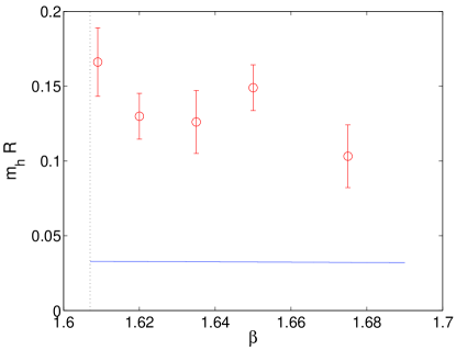
Figure 1: The Higgs mass.

Figure 1 shows the Higgs mass $m_{h}$ in units of $1/R$ as a function of $\beta$. The solid horizontal line corresponds to the 1-loop formula Eq. (7). The first observation we would like to make is that the Higgs mass can be measured without any fine-tuning of the lattice parameters. The second is that it does not diverge as the cut-off is increased by approaching the phase transition. The third observation is that the Higgs mass in units of $1/R$ decreases slowly as we move away from the phase transition.

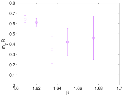
Figure 2: The photon mass.

Figure 2 shows the photon mass $m_{\gamma}$ in units of $1/R$ as a function of $\beta$. Contrary to the 1-loop prediction, it is non-zero, indicating spontaneous symmetry breaking in the pure gauge theory. This is the first non-perturbative evidence for the Higgs mechanism originating from an extra dimension. The photon mass in units of $1/R$ is constant close to the phase transition and decreases at larger $\beta$, where it becomes more difficult to extract. In this simple model the photon mass is larger than the Higgs mass. It would be interesting to see if this is a generic property since in phenomenological applications one would like the Higgs to be heavier than the vector bosons.

V The static potential

In this section we discuss the results for the static potential in the four-dimensional slices. Simulations were performed on lattices of sizes $T/a=32$, $L/a=16$, and $N_{5}=6$. The statistics is 4000 measurements.

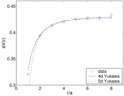
Figure 3: U(1) static potential at the boundary.

Figure 3 shows the static potential on the boundary slice $n_{5}=0$ for $\beta=1.609$. Since the photon mass is non-zero, fits to four- ($-c_{1}\exp(-m_{\gamma}r)/r+c_{0}$, solid line) and five- ($-d_{1}K_{1}(m_{\gamma}r)/r+d_{0}$, where $K_{1}$ is a modified Bessel function, dashed line) dimensional Yukawa potentials are performed, using $m_{\gamma}R=0.646$ from Fig. 2. The point at $r/a=1$ is neglected. The data are consistent with spontaneous symmetry breaking and the minimum $\chi^{2}/{\rm dof}=0.35$ is obtained for the four-dimensional Yukawa potential. For the five-dimensional Yukawa potential we get $\chi^{2}/n_{\rm df}=2.6$. Thus the data favour dimensional reduction. Ignoring spontaneous symmetry breaking, acceptable fits to the data are also obtained with a five-dimensional ($-e_{1}/r^{2}+e_{0}$) or a four-dimensional ($-f_{1}/r+f_{0}$) Coulomb form.

The potential in the four-dimensional slices in the bulk has larger errors and can be fitted equally well to any of the potential forms mentioned above.