CERN-PH-TH-2006-007

hep-lat/0602005

QCD at Zero Baryon Density
and the Polyakov Loop Paradox

Slavo Kratochvila^a, and Philippe de Forcrand^ab,

^aInstitute for Theoretical Physics, ETH Zürich, CH-8093 Zürich, Switzerland
^bCERN, Physics Department, TH Unit, CH-1211 Geneva 23, Switzerland

Abstract
We compare the grand canonical partition function at fixed chemical potential $\mu$ with the canonical partition function at fixed baryon number $B$, formally and by numerical simulations at $\mu=0$ and $B=0$ with four flavours of staggered quarks. We verify that the free energy densities are equal in the thermodynamic limit, and show that they can be well described by the hadron resonance gas at $T<T_{c}$ and by the free fermion gas at $T>T_{c}$.
Small differences between the two ensembles, for thermodynamic observables characterising the deconfinement phase transition, vanish with increasing lattice size. These differences are solely caused by contributions of non-zero baryon density sectors, which are exponentially suppressed with increasing volume. The Polyakov loop shows a different behaviour: for all temperatures and volumes, its expectation value is exactly zero in the canonical formulation, whereas it is always non-zero in the commonly used grand-canonical formulation. We clarify this paradoxical difference, and show that the non-vanishing Polyakov loop expectation value is due to contributions of non-zero triality states, which are not physical, because they give zero contribution to the partition function.

1 Introduction

To simulate QCD thermodynamics on the lattice [1], one commonly uses the grand canonical partition function with respect to the quark number as a function of a chemical potential $\mu$. It is given, after integration over the fermion fields, by

$$Z_{GC}(T,\mu)=\int[DU]\;e^{-S_{g}[\beta,U]}\det M(U;\mu)\;.$$ (1)

Recently, another approach using a canonical formalism has been used [2, 3]. The canonical partition function, which will be derived in detail in the next section, is

$$Z_{C}(T,Q)=\int_{-\infty}^{\infty}d\left(\frac{\mu_{I}}{T}\right)\;e^{-iQ\frac{\mu_{I}}{T}}Z_{GC}(T,\mu=i\mu_{I})\;.$$ (2)

The physics described by both ensembles, grand-canonical and canonical, must be the same in the thermodynamic limit, ie. the free energy density should be the same. This has been shown in Ref. [4, 5], and will be confirmed in this study. It is thus puzzling that the Polyakov loop expectation value in the canonical ensemble is exactly zero, while it is non-zero in the grand-canonical ensemble, for all temperatures and volumes. We will show that this discrepancy is due to contributions from the canonical sectors with a quark number that is not a multiple of three: the so-called non-zero triality sectors. Discussions on the role of these non-zero triality sectors have a long history [6] and include speculations that their influence persists even in the thermodynamic limit, so that they must be explicitly projected out. It is our purpose to clarify these issues.

In the following, we discuss properties of the grand canonical partition function as a function of an imaginary chemical potential and construct the canonical partition function (Section II). We then show that the Polyakov loop vanishes in the canonical ensemble (Section III), and resolve the paradox above (Section IV). After presenting our numerical method to simulate the zero baryon density sector, which is the first step towards finite density QCD simulations (Section V), we elaborate on the results for the free energy density as a function of the imaginary chemical potential, which we compare with predictions of the hadron resonance gas model [7] and of a free fermion gas (Section VI). We further study the expectation values and finite size effects of thermodynamic observables, like the plaquette and the chiral condensate in both formulations (Section VII). Conclusions follow. Preliminary results of this study have been presented in Ref. [5].

2 Canonical Ensemble

Let us first discuss symmetries of the grand canonical partition function $Z_{GC}(T,\mu)$ as a function of an imaginary chemical potential $\mu=i\mu_{I}$, following Ref. [8]:

• Evenness: $Z_{GC}(-i\mu_{I})=Z_{GC}(+i\mu_{I})$.
  The transformation $\mu\to-\mu$ can be compensated by time-reversal, ie. by interchanging particles and anti-particles. Time reversal is equivalent to CP symmetry (since CPT is always a good symmetry), and thus does not change the thermodynamics in the absence of CP violating terms.

• $\frac{2\pi T}{3}$-periodicity in $\mu_{I}$: ${Z_{GC}(i(\mu_{I}+\frac{2\pi T}{3}))}=Z_{GC}(i\mu_{I})$.
  A shift in the imaginary chemical potential $\mu_{I}\to\mu_{I}+\frac{2\pi k}{3}T$ can be exactly compensated by a $Z_{3}$-transformation, ie. by a rotation of the Polyakov loop $Pol({\vec{x}})\to e^{-i\frac{2\pi k}{3}}Pol({\vec{x}})$, configuration by configuration. Since the path integral sums over all possible gauge fields, the partition function stays the same.

These properties lead to an expectation for the phase structure in the $T-\mu_{I}$ plane, see Ref. [8] and Fig. 1. In the low-temperature phase where the $Z_{3}$-symmetry is realised (“disordered”), the periodicity in $\mu_{I}$ is smoothly realised. However, at high temperature, this $Z_{3}$-symmetry is spontaneously broken in favor of one of the $Z_{3}$-sectors (“ordered”). Which sector is preferred depends on $\mu_{I}$. Thus, the existence of $Z_{3}$-sectors forces the appearance of phase transitions at high temperature. By symmetry, these discontinuities must appear at $\mu_{I}=\frac{2\pi kT}{3}+\frac{\pi T}{3}$. The transitions are first-order since the derivative of the free energy with respect to $\mu_{I}$ is discontinuous.

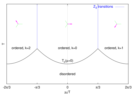
Figure 1: Phase diagram of $Z_{GC}(i\mu_{I})$ in the $(\mu_{I},T)$ plane. The arrows indicate the orientation of the Polyakov loop. The vertical lines mark the “order-order” $Z_{3}$ transitions, which are first-order. Properties of the “order-disorder” $Z_{3}$ transitions (curved lines) depend on the parameters (number of flavours, quark masses) of the theory.

To obtain the canonical partition function $Z_{C}(T,Q)$, we fix to $Q$ the conserved charge $\hat{N}=\int d^{3}\vec{x}\;\bar{\psi}(\vec{x})\;\gamma_{0}\;\psi(\vec{x})$, which represents the net quark number. This is accomplished by inserting a $\delta$-function in the grand canonical partition function:

$$Z_{C}(T,Q)=\int[DU][D\bar{\Psi}][D\Psi]\;e^{-S_{g}[U;T]-S_{F}[U,\bar{\Psi},\Psi;T]}\delta\left(\hat{N}-Q\right)\;.$$ (3)

The $\delta$-function admits a Fourier representation with the new variable $\bar{\mu}_{I}$:

$$Z_{C}(T,Q) =\mathcal{N}\int_{-\infty}^{\infty}d\bar{\mu}_{I}e^{-iQ\bar{\mu}_{I}}\times\int[DU][D\bar{\Psi}][D\Psi]\;e^{-S_{g}[U;\beta]-S_{F}[U,\bar{\psi},\psi]+i\bar{\mu}_{I}\hat{N}}$$

$$=\mathcal{N}\int_{-\infty}^{\infty}d\bar{\mu}_{I}e^{-iQ\bar{\mu}_{I}}\times\int[DU][D\bar{\Psi}][D\Psi]\;\times$$

$$\qquad\qquad\times e^{-S_{g}[U;\beta]-S_{F}[U,\bar{\psi},\psi]+i\bar{\mu}_{I}\int d^{3}\vec{x}\;\bar{\psi}(\vec{x})\;\gamma_{0}\;\psi(\vec{x})}$$

$$=\mathcal{N}\int_{-\infty}^{\infty}d\bar{\mu}_{I}e^{-iQ\bar{\mu}_{I}}\times\int[DU][D\bar{\Psi}][D\Psi]\;\times$$

$$\qquad\qquad\times e^{-S_{g}[U;\beta]-S_{F}[U,\bar{\psi},\psi]+i\bar{\mu}_{I}T\int_{0}^{\frac{1}{T}}d\tau\int d^{3}\vec{x}\;\bar{\psi}(\vec{x})\;\gamma_{0}\;\psi(\vec{x})}\;.$$ (4)

where $\mathcal{N}$ is a normalisation factor. In the last line, we have used the fact that $Q$ is conserved.

One recognises $i\mu_{I}=i\bar{\mu}_{I}T$ as an imaginary chemical potential, so that

$$Z_{C}(T,Q)=\mathcal{N}\int_{-\infty}^{\infty}d\bar{\mu}_{I}e^{-iQ\bar{\mu}_{I}}Z_{GC}(T,i\bar{\mu}_{I}T)=\frac{3}{2\pi}\int_{-\frac{\pi}{3}}^{\frac{\pi}{3}}d\bar{\mu}_{I}e^{-iQ\bar{\mu}_{I}}Z_{GC}(T,i\bar{\mu}_{I}T)\;,$$ (5)

where we have exploited the $\frac{2\pi T}{3}$-periodicity in $\mu_{I}$ of $Z_{GC}(i\mu_{I})$ in the last step. From this periodicity, it follows that $Z_{C}(T,Q)=0$ except for $\frac{Q}{3}\equiv B\in{\mathbb{Z}}$, where $B$ is the baryon number. The canonical partition function vanishes for non-integer baryon number, i.e. for non-zero triality sectors. Note that our argument does not rely on particular spatial boundary conditions. The same conclusion holds for periodic or, for example, $C$-periodic spatial b.c., even though the latter break the $Z(3)$ symmetry. For convenience, we write

$$Z_{C}(T,B)=\frac{1}{2\pi}\int_{-\pi}^{\pi}d\left(\frac{\mu_{I}}{T}\right)e^{-i3B\frac{\mu_{I}}{T}}Z_{GC}(T,i\mu_{I})\;.$$ (6)

Now, the fugacity expansion allows us to go back from the canonical partition functions to the grand canonical one:

$$Z_{GC}(T,\mu)=\sum_{Q=-\infty}^{+\infty}e^{Q\frac{\mu}{T}}Z_{C}(T,Q)\;.$$ (7)

This expression is identical to Eq.(1), as can be seen by substituting (5) for $Z_{C}(T,Q)$ above and summing over $Q$ first. However, we can remove from the sum the non-zero triality (fractional $B$) sectors, since each of them gives a zero contribution, thus obtaining:

$$Z_{GC}(T,\mu)=\sum_{B=-\infty}^{\infty}e^{3B\frac{\mu}{T}}Z_{C}(T,B)\;.$$ (8)

Let us stress again that this grand canonical partition function is identical with the one given in Eq.(1). The two expressions differ by the inclusion of non-zero triality sectors, which we just showed are zero. However, these zero contributions are explicitly projected out in (8) [6]. In the following, we will come back to this and consider the effect of this projecting out on the $Z_{3}$-sensitive Polyakov loop.

3 Polyakov Loop in the Canonical Ensemble

The expectation value of the Polyakov loop in the canonical ensemble is zero for all temperatures and volumes. We show this explicitly as follows. The chemical potential is introduced on the lattice as an external imaginary gauge field

$$U_{4}(x)\to e^{+\mu a}U_{4}(x)$$ (9)

$$U^{\dagger}_{4}(x)\to e^{-\mu a}U^{\dagger}_{4}(x)\;,$$ (10)

or equivalently as

$$U_{4}({\vec{x}},x_{4}=x_{4_{0}})\to e^{+N_{t}\mu a}U_{4}({\vec{x}},x_{4}=x_{4_{0}})$$ (11)

$$U^{\dagger}_{4}({\vec{x}},x_{4}=x_{4_{0}})\to e^{-N_{t}\mu a}U^{\dagger}_{4}({\vec{x}},x_{4}=x_{4_{0}})\;,$$ (12)

on a given temporal hyperplane $x_{4_{0}}$. An imaginary chemical potential $i\mu_{I}=i\frac{2\pi Tk}{3}$ can then be absorbed in a $Z_{3}$ centre transformation

$$U_{4}({\vec{x}},x_{4}=x_{4_{0}})\to e^{iN_{t}a\frac{2\pi Tk}{3}}U_{4}(x)=z(k)U_{4}({\vec{x}},x_{4}=x_{4_{0}})\;.$$ (13)

with $z(k)\equiv e^{i\frac{2\pi k}{3}}\;\mathbbm{1}_{3}$. As a consequence, the two configurations $\{U,\mu_{I}\}$ and $\{z(k)U,\mu_{I}-\frac{2\pi Tk}{3}\}$ have the same value for the Dirac determinant $\det M(U;\mu_{I})=\det M(z(k)U;\mu_{I}-\frac{2\pi Tk}{3})$, but the Polyakov loop is centre-rotated. We can then group the configurations of a canonical ensemble in triplets having $Z_{3}$-rotated Polyakov loop:

$$Z_{C}(T,B)=\frac{1}{2\pi}\int_{-\pi}^{\pi}d\left(\frac{\mu_{I}}{T}\right)\;e^{-i3B\frac{\mu_{I}}{T}}\int[DU]\;e^{-S_{g}[U;\beta]}\;\frac{1}{3}\sum_{k=0}^{2}\det M(z(k)U_{4}(x_{4}=x_{4_{0}}),\mu_{I})\;,$$ (14)

The three members of a triplet give identical contributions to $Z_{C}(T,B)$, since $\det M(z(k)U;\mu_{I})=\det M(U;\mu_{I}+\frac{2\pi Tk}{3})$ and $e^{-i3B\frac{1}{T}\frac{2\pi Tk}{3}}=1$ for $B\in\mathbb{Z}$. In Fig. 2, we show the distribution of the Polyakov loop, where the $Z_{3}$ symmetry (and hence the triplets) is clearly visible in the canonical ensemble (bottom). In each triplet, the average of the Polyakov loops is $Pol_{i}\times\left(1+e^{-i\frac{2\pi}{3}}+e^{i\frac{2\pi}{3}}\right)=0$, and therefore the ensemble average also vanishes:

$$\langle Pol\rangle_{Z_{C}(T,B)}=0$$ (15)

for any integer baryon number and temperature. Note again that the argument does not depend on a particular choice of spatial boundary conditions.

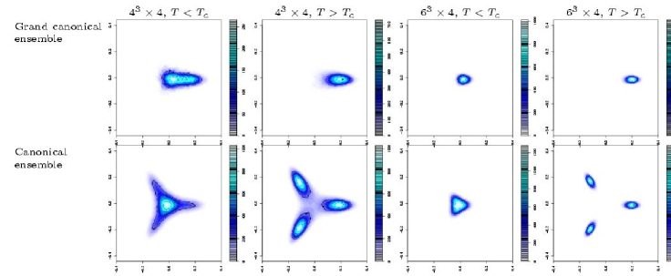
Figure 2: Distribution of the complex Polyakov loop trace in the grand canonical (top) and canonical (bottom) ensembles. left: $4^{3}\times 4$, right: $6^{3}\times 4$. In the thermodynamic limit, the distributions agree for both ensembles, up to two additional $Z_{3}$-rotations in the canonical ensemble.

4 Polyakov Loop in the Grand Canonical Ensemble

In the ensemble generated by the grand canonical partition function Eq.(1)

$$Z_{GC}(T,\mu)=\int[DU]e^{-S_{g}[U;\beta]}\det M(U;\mu)\;,$$ (16)

the fermion determinant explicitly breaks the $Z_{3}$ symmetry, so that the expectation value of the Polyakov loop

$$\langle Pol\rangle_{Z_{GC}(T,\mu)}\neq 0$$ (17)

is non-zero for any chemical potential, temperature and volume. In the following, we show that this non-vanishing value is caused by canonical sectors with quark numbers which are not a multiple of three.

We express the grand canonical partition function via the fugacity expansion in the quark number $Q$ (we take $\mu=0$ for notational simplicity only; the argument holds for any $\mu$):

$$Z_{GC}(T,\mu=0) =\sum_{Q}Z_{C}(T,Q)\text{\;\;with\;\;}Z_{C}(T,Q)=0\text{\;\;if\;\;}Q\neq 0\;\text{mod}\;3$$

$$=...+Z_{C}(0)+Z\!\!\!\!\boldmath{\times}\!\!\!\,\,_{C}(1)+Z\!\!\!\!\boldmath{\times}\!\!\!\,\,_{C}(2)+Z_{C}(3)+Z\!\!\!\!\boldmath{\times}\!\!\!\,\,_{C}(4)+...\;,$$ (18)

where $Z\!\!\!\!\boldmath{\times}\!\!\!\,\,_{C}(\cdot)$ indicates $Z_{C}(\cdot)=0$. The canonical partition functions can be written as $Z_{C}(T,Q)=\sum_{i}W_{i}(Q)$, where $i$ labels each configuration, and $W_{i}(Q)$ is the corresponding Boltzmann weight. The expectation value of the Polyakov loop is then generically given by

$$\langle Pol\rangle_{GC} =\frac{\sum_{Q}\text{\;Num}(Q)}{Z_{GC}(T,\mu=0)}$$ (19)

$$=\frac{...+\text{\;Num}\!\!\!\!\!\!\boldmath{\times}\!\,\,(0)+\text{\;Num}(1)+\text{\;Num}(2)+\text{\;Num}\!\!\!\!\!\!\boldmath{\times}\!\,\,(3)+\text{\;Num}(4)+..}{...+Z_{C}(0)+Z\!\!\!\!\boldmath{\times}\!\!\!\,\,_{C}(1)+Z\!\!\!\!\boldmath{\times}\!\!\!\,\,_{C}(2)+Z_{C}(3)+Z\!\!\!\!\boldmath{\times}\!\!\!\,\,_{C}(4)+...}\neq 0\;,$$

where $\textnormal{Num}(Q)=\sum_{i}Pol_{i}W_{i}(Q)$, which vanishes if $Q$ is a multiple of 3 due to Eq.(15). It follows that the contributions of canonical sectors with fractional baryon number to the Polyakov loop are unphysical, since the corresponding canonical expectation value is infinite:

$$\langle Pol\rangle_{Z_{C}(T,Q\neq 0\;\text{mod}\;3)}=\frac{\text{\;Num}(Q\neq 0\;\text{mod}\;3)}{Z\!\!\!\!\boldmath{\times}\!\!\!\,\,_{C}(Q\neq 0\;\text{mod}\;3)}=\frac{\text{non-zero}}{0}=\infty\;.$$ (20)

This argument makes it clear that the expectation value of the Polyakov loop is non-zero for all temperatures and volumes, if we use the grand canonical partition function with respect to the quark number, see Eq.(1) and Fig. 2, top row. However, if we use the grand canonical partition function with respect to the baryon number, see Eq.(8), the expectation value of the Polyakov loop will be exactly zero even in this equivalent grand canonical formulation.

Thus, the physical meaning of the $Z_{3}$-sensitive Polyakov loop expectation value is rather limited. It is the $Z_{3}$-invariant correlator $\langle Pol(0)Pol(x)^{\dagger}\rangle$ which is physical, and indicates confinement or deconfinement by its $|x|\to\infty$ limit. In the canonical ensemble, this limit is not equal to $|\langle Pol\rangle|^{2}$, which is identically zero: the clustering property is not satisfied. This is evidence of spontaneous breaking of the center symmetry in the presence of fermions. The symmetry is broken spontaneously at all temperatures and densities, rather than explicitly as in the usual grand canonical ensemble.

5 Numerical Approach to Zero Baryon Density

In order to design an algorithm that is able to measure an observable as a function of the quark, or rather baryon number, we need to understand how the expectation value of an observable $\hat{O}$ can be evaluated in the canonical ensemble. It is given by

$$\langle\hat{O}\rangle_{B}\equiv\frac{\frac{1}{2\pi}\int_{-\pi}^{\pi}\;d\bar{\mu}_{I}\;e^{-i3B\bar{\mu}_{I}}\int[DU]\;e^{-S_{g}[U;\beta]}\det M(U;i\mu_{I}=i\bar{\mu}_{I}T)\;\hat{O}(U)}{Z_{C}(T,B)}\;.$$ (21)

We recognise the following numerical description. We treat $\bar{\mu}_{I}$ as a dynamical degree of freedom, and supplement the ordinary Monte Carlo (Hybrid MC, R-algorithm, PHMC, RHMC, $\ldots$) at fixed $\bar{\mu}_{I}$ with a noisy Metropolis update of $\bar{\mu}_{I}\rightarrow\bar{\mu}_{I}^{\prime}$ keeping the configuration $\{U\}$ fixed. Thus, we alternate two kinds of Metropolis steps.

1. Update of the links by standard Hybrid Monte Carlo [9]:
   Keeping the imaginary chemical potential $\mu_{I}$ fixed, we propose a new configuration $\{U^{\prime}\}$, obtained by leapfrog integration of Hamilton’s equations, as a Metropolis candidate. It is then accepted with the ordinary Metropolis probability

   $$Prob(U\to U^{\prime})=\min\left(1,e^{-\Delta S}\right)\;,$$ (22)

   where $\Delta S$ is the difference between the action of $\{U^{\prime}\}$ and that of $\{U\}$.

2. Metropolis update of the imaginary chemical potential by a noisy estimator:
   Keeping the gauge field configuration $\{U\}$ fixed, we propose a new imaginary chemical potential $\mu_{I}^{\prime}$, obtained from $\mu_{I}$ by a random step drawn from an even distribution. The update is based on the acceptance

   $$\textnormal{Prob}(\mu_{I}\rightarrow\mu_{I}^{\prime})=\min\left(1,\frac{e^{-i3B\bar{\mu}_{I}^{\prime}}\det^{N_{f}}(\mbox{$D$\kern-6.49994pt\hbox{/}\hskip 2.5pt}(\mu_{I}^{\prime})+m)}{e^{-i3B\bar{\mu}_{I}}\det^{N_{f}}(\mbox{$D$\kern-6.49994pt\hbox{/}\hskip 2.5pt}(\mu_{I})+m)}\right)\;.$$ (23)

   The ratio of determinants is evaluated with a stochastic estimator (see Appendix Appendix: Stochastic Estimator), namely

   $$\frac{\det^{N_{f}}(\mbox{$D$\kern-6.49994pt\hbox{/}\hskip 2.5pt}(\mu_{I}^{\prime})+m)}{\det^{N_{f}}(\mbox{$D$\kern-6.49994pt\hbox{/}\hskip 2.5pt}(\mu_{I})+m)}=\langle e^{-|(\not\kern-0.20999ptD(\mu_{I}^{\prime})+m)^{-N_{f}/2}(\not\kern-0.20999ptD(\mu_{I})+m)^{N_{f}/2}\eta|^{2}+|\eta|^{2}}\rangle_{\eta}$$ (24)

   where $\eta$ is a Gaussian complex vector. Since one Gaussian vector is sufficient, the computational overhead is negligible.

The algorithm above allows the sampling of any positive measure in $\mu_{I}$. However, the oscillatory part $e^{-i3B\bar{\mu}_{I}}$ in the sampling weight causes a sign problem for non-zero baryon number $B$. One can use $|\cos(3B\bar{\mu}_{I})|$ as a sampling measure and fold the remaining sign in the observable. But such an approach breaks down for rather small $B$ already [10]. Nevertheless, at $B=0$, $e^{-i3B\bar{\mu}_{I}}|_{B=0}=1$ and thus, the Boltzmann weight is real and positive. Thus, this simple algorithm suits our purpose here. To help ergodicity, we can also perform a “$Z_{3}$-move” at any time:

$${\mu_{I}\to\mu_{I}\pm\frac{2\pi T}{3}} {U_{4}(\vec{x},x_{4}=x_{4_{0}})\to U_{4}(\vec{x},x_{4}=x_{4_{0}})e^{\mp i\frac{2\pi}{3}},\;\forall\vec{x}}\;,$$ (25)

where $U_{4}(\vec{x},x_{4}=x_{4_{0}})$ are the temporal links at a given time-slice $x_{4_{0}}$. Such a “$Z_{3}$-move” is always accepted, since the configuration $\{U,\mu_{I}\}$ and the one with a centre-rotated Polyakov loop, but shifted imaginary chemical potential, $\{U\times e^{-i\frac{2\pi}{3}},\mu_{I}+\frac{2\pi T}{3}\}$ have the same Dirac determinant, and thus the same sampling weight, as discussed at length in section 3.

A computational detail: For $T>T_{c}$, the $\mu_{I}$-distribution is sharply peaked around $0,\pm\frac{2\pi T}{3}$. To sample this distribution accurately in the whole interval, we apply a multicanonical algorithm in the $T>T_{c}$ regime for the larger lattices ($6^{3}\times 4$ and $8^{3}\times 4$) [11]. For this, we bias the sampling of the imaginary chemical potential by modifying the acceptance probability

$$\textnormal{Prob}^{\textnormal{multi}}(\mu_{I}\rightarrow\mu_{I}^{\prime})=\min\left(1,\frac{\det^{N_{f}}(\mbox{$D$\kern-6.49994pt\hbox{/}\hskip 2.5pt}(\mu_{I}^{\prime})+m)}{\det^{N_{f}}(\mbox{$D$\kern-6.49994pt\hbox{/}\hskip 2.5pt}(\mu_{I})+m)}\;e^{(bias(\mu_{I}^{\prime})-bias(\mu_{I}))}\right)\;,$$ (26)

with $bias(\mu_{I})$ chosen such that the sampled histogram becomes flat for all $\mu_{I}$. The expectation value of an observable $\hat{O}$ is then given by

$$\langle\hat{O}\rangle=\frac{1}{\sum_{\{U;\mu_{I}\}}e^{-bias(U;\mu_{I})}}\sum_{\{U;\mu_{I}\}}\hat{O}(U;\mu_{I})e^{-bias(U;\mu_{I})}\;,$$ (27)

where $\{U;\mu_{I}\}$ labels the configurations $\{U\}$ sampled at imaginary chemical potential $\mu_{I}$.

We focus on four flavours of Kogut-Susskind fermions with degenerate mass $am=0.05$ and lattices with $N_{t}=4$ time-slices, i.e. $\frac{m}{T}=0.2$. With these parameters, the zero-temperature pion mass is about 350 MeV [12]. Simulations are performed on lattices with spatial extents $4^{3}$, $6^{3}$ and $8^{3}$ at seven temperatures, ranging from $\frac{T}{T_{c}}=0.85$ to $1.1$, with good overlap between the “neighbouring” ensembles. We analyse the results using Ferrenberg-Swendsen reweighting [13].

6 Free Energy Density

In the grand canonical ensemble, the change of the free energy density with chemical potential $\mu$ (as a dimensionless quantity) is given in terms of the partition function

$$\frac{\Delta F(T,\mu)}{VT^{4}}\equiv-\frac{1}{VT^{3}}\log\frac{Z_{GC}(T,\mu)}{Z_{GC}(T,0)}\;.$$ (28)

A standard approach [14, 16] is to perform a Taylor expansion in $\mu$ about $\mu=0$, where the derivatives entering the series may be expressed as complicated expectation values evaluated at $\mu=0$. Remember that this expansion is in even powers of $\mu$, since $Z_{GC}(\mu)=Z_{GC}(-\mu)$. In our approach, the free energy density comes for free from the $\mu_{I}$-histogram in the canonical simulation, and moreover, to all orders. At low temperature, however, the histograms are quite noisy. Therefore we will, when needed, use results from the more sophisticated method [3], where we can calculate the grand canonical partition function for an arbitrary imaginary chemical potential as a consequence of the reweighting method that we apply.

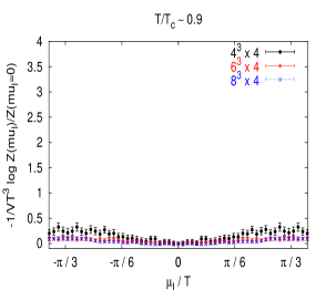
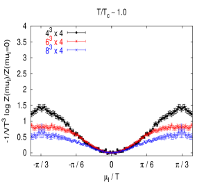
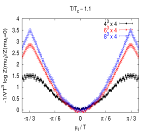
Figure 3: $\frac{\Delta F(T,\mu_{I})}{VT^{4}}$ as a function of $\frac{\mu_{I}}{T}$, at temperatures $\frac{T}{T_{c}}\sim 0.9,\;1.0,\;1.1$ from left to right. The free energy density varies much more upon entering the high-temperature phase, and the $Z_{3}$ first-order transitions become visible (right).

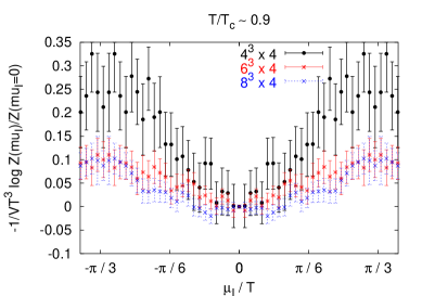
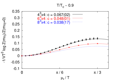
Figure 4: $\frac{\Delta F(T,\mu_{I})}{VT^{4}}$ as a function of $\frac{\mu_{I}}{T}$ for $\frac{T}{T_{c}}\sim 0.9$. The histogram method is very noisy. We show (left) a rescaled version of the leftmost plot in Fig. 3. We also present (right) results based on a reweighting method with variance reduction [3]. The results are in agreement with the histogram method, but allow for a more reliable description by a Fourier expansion. One Fourier coefficient suffices to describe the data points. The reweighting method [3] calculation is computationally demanding and has not been performed yet for the $8^{3}\times 4$ lattice. We thus only draw the fit, which is based on histogram data.

In Fig. 3 we show the free energy divided by $VT^{4}$ versus $\frac{\mu_{I}}{T}$ for $\frac{T}{T_{c}}<1$, $\frac{T}{T_{c}}\simeq 1$ and $\frac{T}{T_{c}}>1$. In all cases, we observe a minimum at $\frac{\mu_{I}}{T}=0$. Therefore, in the thermodynamic limit, only $\frac{\mu_{I}}{T}=0\mod\frac{2\pi}{3}$ will survive. This establishes numerically the expected equivalence of $Z_{C}(T,B=0)$ with $Z_{GC}(T,\mu=0)$.

For $\frac{T}{T_{c}}\sim 0.9$, no singularities develop at $\frac{\mu_{I}}{T}=\pm\frac{\pi}{3}$ in the thermodynamic limit, thus indicating a crossover, as expected from the phase diagram $T$-$\mu_{I}$, Fig. 1. In Fig. 4, (left), we show the free energy density, determined by the histogram method, which is very flat and noisy unfortunately. The periodicity of the free energy density is $\frac{2\pi T}{3}$, and we exploit it by a Fourier expansion in $3k\frac{\mu_{I}}{T}$ using the Ansatz

$$\frac{\Delta F(T,\mu_{I})}{VT^{4}}=c\left(1-\cos(3\frac{\mu_{I}}{T})\right)+d\cos(6\frac{\mu_{I}}{T})+\ldots\;.$$ (29)

In order to improve the determination of the coefficients $c$,$d$,$\ldots$, we use results based on the reweighting method described in Ref. [3]. Within errors, the free energy density is in agreement with the histogram method, but with much smaller statistical uncertainty. The fit is excellent already with one Fourier coefficient, with no indication for higher Fourier components, at least on the small lattices we consider.

In the hadron resonance gas model (see Ref. [17] for a detailed discussion), the partition function can be split into mesonic and baryonic contributions. Since we are interested in the dependency on a baryon chemical potential $\mu_{B}=3\mu$, it is sufficient to study the baryonic part only. In the limit $m_{B}\gg T,\mu_{B}$, where $m_{B}$ corresponds to the baryonic resonance mass, the Ansatz for the free energy density as a function of an imaginary chemical potential is

$$\frac{F(T,\mu_{I})}{VT^{4}}-\frac{F(T,0)}{VT^{4}}\equiv\frac{\Delta F(T,\mu_{I})}{VT^{4}}=f(T)(1-\cos(\frac{3\mu_{I}}{T}))\;,$$ (30)

where $f(T)\equiv\frac{1}{\pi^{2}}\sum_{i\in\mathrm{Baryons}}\left(\frac{m_{i}}{T}\right)^{2}K_{2}\left(\frac{m_{i}}{T}\right)$. We thus have a mean to measure the sum of resonances $f(T)$. For example in the case of a $6^{3}\times 4$ lattice, we find $f(T\sim 0.9T_{c})=0.048(1)$. Our data can be well described by this Ansatz. This confirms our expectation that the relevant degrees of freedom in the low-temperature phase are hadrons. The masses of these hadrons are much larger than the scale given by the temperature, since the free energy density changes only slightly when varying the imaginary chemical potential, thus $m_{H}\gg\mu_{I}\sim T_{c}\approx 160$ MeV.

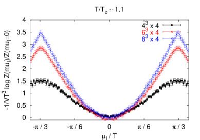
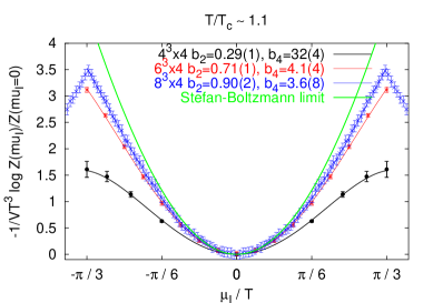
Figure 5: $\frac{\Delta F(T,\mu_{I})}{VT^{4}}$ as a function of $\frac{\mu_{I}}{T}$ for $\frac{T}{T_{c}}\sim 1.1$. (left) The histogram method; (right) the reweighting method [3], supplemented by the histogram results for $8^{3}\times 4$. A simple modification of the free gas expression describes all the data. As the volume increases, the data come close to the Stefan-Boltzmann limit ($T\to\infty$) even though $\frac{T}{T_{c}}\sim 1.1$ only.

For $\frac{T}{T_{c}}\sim 1.1$ we expect a cusp at $\mu_{I}=\pm\frac{\pi T}{3}$ ($Z_{3}$-transitions) to develop in the thermodynamic limit, due to the first order phase transition. Indeed, it appears clearly as the volume increases, see Fig. 5 for a comparison of the histogram results (left) versus the reweighting approach (right).

We can try to describe these results by a generic Taylor series in $\frac{\mu_{I}}{T}$ as an Ansatz, which can be compared with a simple model at high temperature, the free gas of massless quarks. If we perform an analytic continuation from real to imaginary chemical potential, then the free energy density of this model is given by

$$\frac{\Delta F(T,\mu_{I})}{VT^{4}}=\frac{N_{f}}{2}\left(\frac{\mu_{I}}{T}\right)^{2}-\frac{N_{f}}{4\pi^{2}}\left(\frac{\mu_{I}}{T}\right)^{4}\;.$$ (31)

These simple expressions are valid in the continuum theory at very high temperature, where the coupling $g(T)\approx 0$. On the lattice we expect finite size corrections ($N_{s}<\infty$) as well as cut-off corrections ($T=\frac{1}{aN_{t}}$). Ref. [16] has calculated the free energy of free fermions on a lattice having infinite spatial size ($N_{s}=\infty$) but finite temporal extent ($N_{t}=4$). Here, we also determine the corrections for finite spatial size $N_{s}=4,6,8,10$ for the free massless fermion gas on the lattice. We set the gauge fields $A_{\mu}(x)=0$, ie. the gauge links to the identity, and solve for the free energy via

$$\frac{\Delta F^{free}_{latt}(T,\mu_{I})}{VT^{4}} =-\frac{\log Z^{free}(T,\mu_{I})}{VT^{3}}=-\frac{\log\det M^{free}(T,\mu_{I})}{VT^{3}}$$

$$\approx C_{2}\frac{N_{f}}{2}\left(\frac{\mu_{I}}{T}\right)^{2}-C_{4}\frac{N_{f}}{4\pi^{2}}\left(\frac{\mu_{I}}{T}\right)^{4}\;.$$ (32)

where $C_{2}$ and $C_{4}$ are fit coefficients. Table 1 summarises the results.

Lattice	$C_{2}$	$C_{4}$	$[C_{6}]$
$4^{3}\times 4$	4.387(1)	0.28(3)	[-]
$6^{3}\times 4$	2.628(1)	1.70(5)	[0.0081(1)]
$8^{3}\times 4$	2.315(1)	2.25(5)	[0.0046(1)]
$10^{3}\times 4$	2.250(1)	2.49(5)	[0.0030(1)]
$\infty^{3}\times 4$	2.25	2.6	-

Table 1: The prediction for the free energy density based on the free massless gas model in the continuum at high temperature suffers from finite size and cut-off effects. The correction terms $C_{2}$ and $C_{4}$ help to quantify the systematics. The functional form in Eq.(32) is sufficient, since the contribution of the additional term $\left(\frac{\mu}{T}\right)^{6}$ is very small.

The coefficients $C_{2}$ and $C_{4}$ approach their infinite volume expectation rather quickly. For the particular quark mass $\frac{m}{T}=0.2$ which we consider, the difference from the massless limit is smaller than the (fitting) errors, and thus, results are not presented explicitly. Note that we have an additional column $[C_{6}]$: we have added the term $C_{6}\left(\frac{\mu}{T}\right)^{6}$ to the Ansatz Eq.(32). The coefficient $C_{6}$ is very small and leaves $C_{2}$ and $C_{4}$ unchanged within the errors.

In the end, we consider the volume-dependent lattice corrections $C_{2}$ and $C_{4}$ and measure the deviation from this free gas model by two parameters $b_{2}(T)$ and $b_{4}(T)$. The Ansatz to describe our results in Fig. 5 is thus

$$\frac{\Delta F(T,\mu_{I})}{VT^{4}}=b_{2}(T)C_{2}\frac{N_{f}}{2}\left(\frac{\mu_{I}}{T}\right)^{2}-b_{4}(T)C_{4}\frac{N_{f}}{4\pi^{2}}\left(\frac{\mu_{I}}{T}\right)^{4}\;.$$ (33)

$T\sim 1.1T_{c}$	$b_{2}(T)$	$b_{4}(T)$	$b_{4}(T)$ (periodic)
$4^{3}\times 4$	0.29(1)	32(4)	7(1)
$6^{3}\times 4$	0.71(1)	4.1(4)	0.2(7)
$8^{3}\times 4$	0.90(2)	3.6(8)	1.4(4)
SB limit ($T\to\infty$)	1	1	1

Table 2: The coefficients of the free energy density expansion for $\frac{T}{T_{c}}\sim 1.1$ come close to their Stefan Boltzmann ($T\to\infty$) value. There are two values for $b_{4}(T)$: the first one is the result of the chi-square fit of Eq.(33); the second one (“periodic”) makes use of a periodicised Ansatz, see Eq.(34). The comparison of the two values gives some measure of the systematic error.

We observe that the leading term approaches the Stefan Boltzmann limit rather fast upon increasing the volume, see Fig. 5 and Table 2. This is somewhat surprising since this coincidence with the Stefan Boltzmann law will occur only at $T\to\infty$. Deviations at $T\sim 1.1\;T_{c}$ should persist even in the thermodynamic limit, reflecting the interactions of the quarks. The reduction of $b_{2}(T)$ from 1 is consistent with leading perturbative corrections [17]. The value we obtain is consistent with that measured in Ref. [19]. The simple prediction of the free massless quark gas model works better than expected. Thus, the relevant degrees of freedom at high temperature are very light quarks, which is also visible in the strong dependency of the free energy density on the imaginary chemical potential, hence $m_{q}\ll\mu_{I}\sim T_{c}\approx 160$ MeV.

The coefficient $b_{4}(T)$ in Table 2 suffers from systematic fitting errors. One source is the fitting range: our Ansatz Eq.(33) does not reflect the $\frac{2\pi}{3}$-periodicity of $\frac{\mu_{I}}{T}$, therefore we are allowed to fit small $\frac{\mu_{I}}{T}$ only. In this regime, the quartic term is subleading and hard to quantify. An estimate of the systematic fitting error can be obtained by varying the fitting range (not explicitly tabulated). Another source is the fitting Ansatz: we could add the next-order term $\left(\frac{\mu_{I}}{T}\right)^{6}$, which changes $C_{4}$ by a few percent, or periodicise the Ansatz by hand via

$$\frac{\Delta F_{per}(T,\mu_{I})}{VT^{4}}=-\frac{1}{VT^{3}}\log\frac{Z_{per}(T,\mu_{I})}{Z_{per}(T,0)}$$ (34)

with

$$Z_{per}(T,\mu_{I})=\sum_{k=-\infty}^{\infty}e^{-VT^{3}\left(b_{2}(T)C_{2}\frac{N_{f}}{2}\left(\frac{\mu_{I}}{T}+\frac{2\pi k}{3}\right)^{2}-b_{4}(T)C_{4}\frac{N_{f}}{4\pi^{2}}\left(\frac{\mu_{I}}{T}+\frac{2\pi k}{3}\right)^{4}\right)}\;.$$ (35)

However, we must truncate (in practice, at $k=\pm 1$) the sum over all sectors to preserve convergence, because of the sign of the $C_{4}$ contribution. In conclusion, we cannot determine $b_{4}(T)$ accurately. Nevertheless, it is remarkable how well the free quark gas model describes our results. On an $8^{3}\times 4$ lattice, the deviation is only about 10%. By using a canonical approach to simulate finite density QCD [3], we can obtain more accurate results, to be presented in a follow-up publication. In particular, we can show that $b_{4}(T=1.1\;T_{c})=2.97(3)$.

7 Deconfinement Transition and Finite Size Effects

The phase transition is signaled by the peak in the susceptibility of the chiral condensate $\langle\bar{\psi}\psi\rangle$ or in the specific heat. In Fig. 6, we show the former.

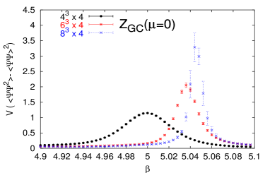
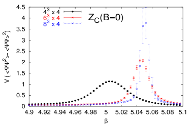
Figure 6: Susceptibility of $\bar{\psi}\psi$ versus $\beta$ for all volumes in the grand canonical and canonical ensembles. left: $Z_{GC}(T,\mu=0)$, right: $Z_{C}(T,B=0)$. Even for the smallest, $4^{4}$, lattice, differences are barely visible.

On the $4^{3}\times 4$ lattice, a slight shift in the pseudo-critical $\beta_{c}$ can be observed between the grand-canonical and the canonical results. It disappears for larger volumes. We observe the same behaviour for the specific heat. The small deviation is caused by contributions from $B\neq 0$ sectors, which are present in the $\mu=0$ ensemble. However they are suppressed by a factor $\sim e^{-B\frac{m_{B}}{T}}\ll 1$, where $m_{B}$ is the mass of a baryon. In terms of the baryon density $\rho$, we recognise the exponential suppression in the volume since $e^{-B\frac{m_{B}}{T}}=e^{-V\rho\frac{m_{B}}{T}}$. Thus, we verify once more that the zero chemical potential ensemble is equivalent to the zero baryon density ensemble in the thermodynamic limit.

Note that the non-zero triality sectors have zero partition function and do not contribute. They do not affect observables studied in this section, which are insensitive to the centre symmetry.

\psfrag{Binder cumulant minimum}{\small min $C_{B}(\hat{O})$}\includegraphics[height=199.16928pt,width=128.0374pt,angle={-90}]{pictures/plaquette_binder_colour.eps}

\psfrag{Binder cumulant minimum}{\small min $C_{B}(\hat{O})$}\includegraphics[height=199.16928pt,width=128.0374pt,angle={-90}]{pictures/chiral_binder_colour.eps}

Figure 7: Binder cumulant minimum versus inverse volume for both ensembles (slightly shifted in the $x$-axis to enhance visibility). left: $\hat{O}=$plaquette, right: $\hat{O}=$chiral condensate. The thermodynamic extrapolation does not reach $\frac{2}{3}$ (the upper left corner of the figure), indicating a first order transition. Finite-size effects, reflected in the $1/V$ slope, are equivalent for both ensembles.

In quenched simulations, a $Z_{3}$-symmetrisation of the Polyakov loop is sometimes enforced by hand, which is accompanied by reduced finite size effects [20]. Therefore, we might expect to observe a similar reduction in the canonical formalism as well compared to the grand canonical one. To compare the finite size effects in the two ensembles, we analyse the minimum of the Binder cumulant [21]

$$C_{B}(\hat{O})=1-\frac{1}{3}\frac{\langle\hat{O}^{4}\rangle}{\langle\hat{O}^{2}\rangle^{2}}$$ (36)

versus the inverse volume $1/V$ (see Fig. 7). For both the plaquette and the chiral condensate, the thermodynamic (linear) extrapolation does not tend to $\frac{2}{3}$ - indicative of a first order phase transition, confirming the finding in the literature [22] for our quark masses. However, for each volume, the measured cumulant values agree between the two ensembles within statistical errors, indicating equivalent finite size effects.

8 Conclusions

For all densities, volumes, and (finite) temperatures, the Polyakov loop expectation value is non-zero in the grand canonical ensemble Eq.(1), and zero in the equivalent canonical ensemble Eq.(2). This Polyakov loop paradox has to be considered an artifact of keeping, in the grand canonical ensemble, sectors with quark numbers not multiple of three. These canonical sectors, the so-called non-zero triality sectors, have zero partition function. Thus, the non-vanishing expectation value $\langle Pol\rangle_{Z_{GC}(T,\mu)}$ in the common grand canonical formulation of QCD at finite temperature and density, Eq.(1), is irrelevant for thermodynamic properties. The physically meaningful Polyakov loop correlator $\langle Pol(0)Pol(x)^{\dagger}\rangle$ behaves in the same way in both ensembles.

Because of quantum and thermal fluctuations, $\langle Pol(0)Pol(x)^{\dagger}\rangle$ tends to a non-zero value when $|x|\to\infty$. On the other hand, $\langle Pol\rangle=0$ in the canonical ensemble. Thus, the clustering property is violated, which shows that the center symmetry is spontaneously broken in the canonical ensemble, rather than explicitly broken by the fermion determinant as in the usual grand-canonical ensemble.

Furthermore, an explicitly centre-symmetric grand canonical partition function $Z_{GC}(T,\mu)$, Eq.(8), can be constructed from the canonical partition functions, where the contributions of non-zero triality states are projected out. This partition function will give identical expectation values to the usual $Z_{GC}(T,\mu)$, apart from a vanishing expectation value for the Polyakov loop. Therefore, the non-zero triality states can be included or excluded: the thermodynamic properties of the theory are unchanged.

We have shown this explicitly by comparing the grand canonical ensemble at $\mu=0$ with the canonical ensemble $B=0$. Numerically, we have established the equivalence of $Z_{GC}(\mu=0)$ and $Z_{C}(B=0)$ in the thermodynamic limit by measuring the free energy density as a function of $\mu_{I}$, using the histogram of the imaginary chemical potential distribution. For all temperatures, we observe a minimum at $\frac{\mu_{I}}{T}=0$. At low temperature, the free energy density of the confined phase can be rather well described by the hadron resonance gas, see Eq.(30). We thus have a simple way to determine the sum of resonances $f(T)$. At high temperature, a slightly modified free gas Ansatz, see Eq.(33), allows to account for all data points in the quark-gluon plasma phase. We determine the finite-size and cut-off correction terms $C_{2}$ and $C_{4}$ by calculating the free energy of the free fermion gas on the lattice and find agreement with the literature for $V\to\infty$. By construction, the interaction coefficients $b_{2}(T)$ and $b_{4}(T)$ tend to 1 for high enough temperatures, reproducing the Stefan Boltzmann law. Just above $T_{c}$, the deviation from 1 in the leading coefficient is about 30% on a $6^{3}\times 4$ lattice; on an $8^{3}\times 4$ lattice, this deviation is about 10% only. This near-agreement with a non-interacting gas is unexpected at such comparatively low temperatures.

The approach to the thermodynamic limit is very similar in the canonical ($B=0$) and grand canonical ($\mu=0$) ensembles. The susceptibility of the chiral condensate, or the specific heat, indicate the same pseudo-critical temperature already on small volumes. A small shift, caused by contributions from non-zero baryon sectors, is visible only on the $4^{3}\times 4$ lattice.

The zero-density canonical formulation requires a centre-symmetric simulation of QCD, which can be achieved very simply with negligible computer overhead, by adding to the standard algorithm a single degree of freedom $\mu_{I}$ updated by Metropolis.

We hope to have fully clarified the (un)importance of non-zero triality states, and thus, to have put to rest long-standing speculations. Further connections between the grand-canonical and the canonical formalisms in the context of non-zero chemical potential/density will be the subject of a forthcoming paper.

9 Acknowledgements

We are grateful to O. Jahn, K. Kajantie, F. Karsch, M. P. Lombardo, O. Philipsen, K. Rummukainen, B. Svetitsky, T. Takaishi, D. Toublan and L.G. Yaffe for fruitful discussions and advice.

Appendix: Stochastic Estimator

A ratio of determinants can be estimated using a single Gaussian complex vector:

$$\frac{\det^{N_{f}}(\mbox{$D$\kern-6.49994pt\hbox{/}\hskip 2.5pt}(\mu_{I}^{\prime})+m)}{\det^{N_{f}}(\mbox{$D$\kern-6.49994pt\hbox{/}\hskip 2.5pt}(\mu_{I})+m)} =\frac{\det^{N_{f}}M(\mu_{I}^{\prime})}{\det^{N_{f}}M(\mu_{I})}=\frac{\int d\phi^{\dagger}d\phi e^{-\phi^{\dagger}\frac{1}{M^{N_{f}}(\mu_{I}^{\prime})}\phi}}{\int d\phi^{\dagger}d\phi e^{-\phi^{\dagger}\frac{1}{M^{N_{f}}(\mu_{I})}\phi}}$$ (37)

$$=\frac{\int d\eta^{\dagger}d\eta\;|J(\phi,\eta,\mu_{I})|\;e^{-\eta^{\dagger}M^{N_{f}/2}(\mu_{I})M^{-N_{f}/2}(\mu_{I}^{\prime})M^{-N_{f}/2}(\mu_{I}^{\prime})M^{N_{f}/2}(\mu_{I})\eta}}{\int d\eta^{\dagger}d\eta\;|J(\phi,\eta,\mu_{I})|\;e^{-\eta^{\dagger}\eta}}$$ (38)

where we have substituted $\phi=M^{N_{f}/2}(\mu_{I})\eta$. Note, that in the above notation, the Jacobian $|J(\phi,\eta,\mu_{I})|$ is $\det M^{N_{f}}(\mu_{I})$, which is independent of $\eta$ and cancels out in the ratio:

$$\frac{\det^{N_{f}}(\mbox{$D$\kern-6.49994pt\hbox{/}\hskip 2.5pt}(\mu_{I}^{\prime})+m)}{\det^{N_{f}}(\mbox{$D$\kern-6.49994pt\hbox{/}\hskip 2.5pt}(\mu_{I})+m)} =\frac{\int d\eta^{\dagger}d\eta\;e^{-|M^{-N_{f}/2}(\mu_{I}^{\prime})M^{N_{f}/2}(\mu_{I})\eta|^{2}}e^{-|\eta|^{2}+|\eta|^{2}}}{\int d\eta^{\dagger}d\eta\;e^{-|\eta|^{2}}}$$ (39)

$$=\langle e^{-|M^{-N_{f}/2}(\mu_{I}^{\prime})M^{N_{f}/2}(\mu_{I})\eta|^{2}+|\eta|^{2}}\rangle_{\eta}\;.$$ (40)

$\langle\cdot\rangle_{\eta}$ tells us that $\eta$ has to be sampled with the distribution $\int d\eta^{\dagger}d\eta\ e^{-|\eta|^{2}}$.

References

- [1] Z. Fodor and S. D. Katz, Phys. Lett. B 534, 87 (2002); C. R. Allton et al., Phys. Rev. D 66 (2002) 074507; P. de Forcrand and O. Philipsen, Nucl. Phys. B 642 (2002) 290; M. D’Elia and M. P. Lombardo, Phys. Rev. D 67 (2003) 014505.
- [2] S. Kratochvila and P. de Forcrand, Nucl. Phys. Proc. Suppl. 140 (2005) 514; A. Alexandru, M. Faber, I. Horvath and K. F. Liu, Nucl. Phys. Proc. Suppl. 140 (2005) 517; A. Alexandru, M. Faber, I. Horvath and K. F. Liu, arXiv:hep-lat/0507020.
- [3] S. Kratochvila and P. de Forcrand, PoS LAT2005 (2005) 167.
- [4] V. Azcoiti and A. Galante, Phys. Lett. B 444 (1998) 421.
- [5] S. Kratochvila and P. de Forcrand, Prog. Theor. Phys. Suppl. 153 (2004) 330 [arXiv:hep-lat/0309146].
- [6] M. Oleszczuk and J. Polonyi, Annals Phys. 227 (1993) 76; M. Oleszczuk, Nucl. Phys. B Proc. Suppl. 39 (1995) 471; O. Borisenko, M. Faber and G. Zinovev, Nucl. Phys. B 444 (1995) 563; K. Fukushima, Annals Phys. 304 (2003) 72.
- [7] R. Hagedorn and J. Rafelski, CERN-TH-2947 Invited lecture given at Int. Symp. on Statistical Mechanics of Quarks and Hadrons, Bielefeld, Germany, Aug 24-31, 1980; J. Rafelski and R. Hagedorn, CERN-TH-2969 Invited talk given at Int. Symp. on Statistical Mechanics of Quarks and Hadrons, Bielefeld, West Germany Aug 24-31, 1980.
- [8] A. Roberge and N. Weiss, Nucl. Phys. B 275 (1986) 734.
- [9] S. Duane, A. D. Kennedy, B. J. Pendleton and D. Roweth, Phys. Lett. B 195 (1987) 216.
- [10] M. G. Alford, A. Kapustin and F. Wilczek, Phys. Rev. D 59 (1999) 054502 .
- [11] B. A. Berg and T. Neuhaus, Phys. Rev. Lett. 68 (1992) 9 [arXiv:hep-lat/9202004].
- [12] M. P. Lombardo, private communication.
- [13] A. M. Ferrenberg and R. H. Swendsen, Phys. Rev. Lett. 61 (1988) 2635; A. M. Ferrenberg and R. H. Swendsen, Phys. Rev. Lett. 63 (1989) 1195.
- [14] C. R. Allton et al., Phys. Rev. D 66 (2002) 074507.
- [15] D. Toublan, private communication
- [16] C. R. Allton et al., Phys. Rev. D 68 (2003) 014507.
- [17] C. R. Allton et al., Phys. Rev. D 71 (2005) 054508 [arXiv:hep-lat/0501030].
- [18] G. Boyd, J. Engels, F. Karsch, E. Laermann, C. Legeland, M. Lutgemeier and B. Petersson, Nucl. Phys. B 469 (1996) 419 .
- [19] M. D’Elia and M. P. Lombardo, Phys. Rev. D 70 (2004) 074509; M. D’Elia, F. Di Renzo and M. P. Lombardo, arXiv:hep-lat/0511029.
- [20] G. Martinelli, G. Parisi, R. Petronzio and F. Rapuano, Phys. Lett. B 122, 283 (1983).
- [21] K. Binder, Z. Phys. B 43 (1981) 119.
- [22] M. Fukugita and A. Ukawa, Phys. Rev. Lett. 57 (1986) 503.