Simulations of ${\cal N}=2$ super Yang-Mills theory in two dimensions

Abstract:

We present results from lattice simulations of ${\cal N}=2$ super Yang-Mills theory in two dimensions. The lattice formulation we use was developed in [1] and retains both gauge invariance and an exact (twisted) supersymmetry for any lattice spacing. Results for both $U(2)$ and $SU(2)$ gauge groups are given. We focus on supersymmetric Ward identities, the phase of the Pfaffian resulting from integration over the Grassmann fields and the nature of the quantum moduli space.

1 Introduction

Supersymmetric field theories play a central role in modern theories of particle physics. They offer a possible solution to the gauge hierarchy problem and are often more tractable analytically than their non-supersymmetric counterparts while still exhibiting features like confinement and chiral symmetry breaking [2]. Super Yang-Mills theories are especially interesting because of their possible connection to string and M-theory [3]. One example of this is the conjectured equivalence between $(p+1)$-dimensional super Yang-Mills theory and supergravity containing $Dp$-brane sources [4].

One attractive scenario for embedding the Standard Model in such a theory is to imagine that supersymmetry breaks spontaneously as some gauge coupling becomes large at low energy. Unfortunately various non-renormalization theorems forbid such a spontaneous breaking at any finite order of perturbation theory so one must turn to non-perturbative mechanisms to drive such symmetry breaking.

Of course the lattice furnishes perhaps the only generally applicable way to study non-perturbative dynamics in field theory. However, the difficulties of discretizing supersymmetric theories are well known. Generic naive discretizations of continuum supersymmetric theories do not preserve supersymmetry. Typically quantum corrections then generate a large number of relevant supersymmetry violating interactions whose couplings must be tuned to zero as the lattice spacing is reduced. This is both unnatural and in many cases (especially for models with extended supersymmetry) prohibitively difficult. Various attempts have been made over the last twenty five years to overcome these problems see [5] and [6] and the recent reviews [7, 8, 9].

Quite recently a series of new approaches have been developed which share the common feature of preserving a sub-algebra of the full supersymmetry algebra exactly at finite lattice spacing In the approach pioneered by Kaplan and collaborators [11] the lattice theory is derived by applying a carefully chosen orbifold condition to a supersymmetric matrix model (see also [12, 13, 14, 15]). A second approach proceeds from a reformulation of the theory using ideas drawn from topological field theory [16].. It is this approach that is the focus of this paper. The hope is that the residual exact supersymmetry will protect the theory from dangerous radiative corrections and obviate the need for fine tuning [11, 22, 18, 17].

This technique was initially used for theories without gauge symmetry [19, 20, 21] corresponding to supersymmetric quantum mechanics, the 2D complex Wess-Zumino model and supersymmetric sigma models. An implementation for gauge theories was initially given by Sugino [22]. Important progress was made when Kawamoto and collaborators [23] pointed out the connection between these topological formulations and Kähler-Dirac fermions. This has led to additional lattice formulations which emphasize the geometrical nature of the underlying theory [10] and [1, 24] (Hamiltonian formulations of lattice supersymmetric theories employing Kähler-Dirac fermions were first proposed in [25] and later in [26])

The key starting point in this approach is to construct a new rotation group from a combination of the original rotation group and part of the R-symmetry associated with the extended SUSY. The supersymmetric field theory is then reformulated in terms of fields which transform as integer spin representations of this new rotation group [27, 28, 23]. This process is given the name twisting and in flat space one can think of it as merely an exotic change of variables in the theory. In this process a scalar anticommuting field is always produced associated with a nilpotent supercharge $Q$. Furthermore, as argued in [28, 1] the twisted superalgebra implies that the action rewritten in terms of these twisted fields is generically $Q$-exact. In this case it is straightforward to construct a lattice action which is $Q$-invariant provided only that we preserve the nilpotency of $Q$ under discretization.

In [1] we gave a concrete application of these ideas by constructing a gauge invariant lattice regularization of ${\cal N}=2$ super Yang-Mills theory in two dimensions which was invariant under the twisted scalar supersymmetry and an additional $SO(1,1)$ scaling symmetry. In this paper we present results from the first numerical simulations of this model.

In this initial work we have examined a variety of Ward identities following from the twisted supersymmetry. In the case of $U(2)$ we find generally good agreement with theory for sufficiently large coupling $\beta$. Specifically we do not need to fine tune any additional couplings to see a restoration of the twisted supersymmetry for small lattice spacing. In the case of $SU(2)$ the agreement is even better – we see no statistically significant breaking of the Ward identities even for small $\beta$. Our results for the string tension indicate that the lattice theory possesses a single confining phase. In addition our initial examination of the low lying spectrum appears to indicate the presence of light scalar bound states.

We have also examined the issue of the phase of the Pfaffian induced by integrating over the fermions. Our Monte Carlo simulations have been conducted in the phase quenched ensemble in which this phase is neglected. We present evidence that the distribution of the phase measured in the phase quenched ensemble peaks around zero at large coupling. This corresponds to our expectation that the relevant Pfaffian is indeed real and positive definite in the continuum limit. Remarkably re-weighting with the phase in the usual way does not appear to generate large corrections to the phase quenched results at least in the case of the supersymmetric Ward identities. We have also examined the distribution of the eigenvalues of the scalar fields in the theory. The latter quantity yields information of the nature of the quantum moduli space. We provide strong evidence that the vacuum degeneracy of the classical theory is lifted at the quantum level.

The paper is organized as follows; we first summarize the reformulation of the continuum theory is terms of twisted fields. This twisted theory has a natural mapping to the lattice and we give the lattice action and the action of the twisted supersymmetry on the lattice fields. The details of our numerical algorithm are then described and lead to a presentation of our results both for $U(2)$ and $SU(2)$ gauge groups. A final section summarizes our conclusions and discusses future work.

2 Continuum Twisted Formulation

Consider a theory with ${\cal N}=2$ supersymmetry in two dimensional Euclidean space. Such a theory contains two Majorana supercharges $q^{I}_{\alpha}$ transforming under the global symmetry group $SO(2)\times SO(2)_{R}$ where the subscript corresponds to two dimensional rotations and the superscript describes the behavior under the R-symmetry corresponding to rotating the two Majorana fields into one another.

The basic idea of twisting, which goes back to Witten [27, 23, 28], is to introduce a new rotation group

$$SO(2)^{\prime}={\rm diagonal\;subgroup}(SO(2)\times SO(2)_{R})$$

and to decompose all fields now as representations of this new rotation group. In simple terms what this means is that whenever I do a rotation in the base space by some angle I must do an equal rotation in the R-symmetry space. It is equivalent to treating the two indices $I$ and $\alpha$ as equivalent. Thus the supercharges are to be interpreted as matrices in this twisted picture.

$$q^{I}_{\alpha}\to q_{\alpha\beta}$$ (1)

Such a matrix may then be expanded on a basis of products of 2D gamma matrices

$$q=QI+Q_{\mu}\gamma_{\mu}+Q_{12}\gamma_{1}\gamma_{2}$$ (2)

The fields $(Q,Q_{\mu},Q_{12})$ are called the twisted supercharges. The original SUSY algebra then implies a corresponding twisted algebra which takes the form

$$\{q,q\}_{\alpha\beta}=4\gamma^{\mu}_{\alpha\beta}p^{\mu}\\$$ (3)

In components this reads

$$\{Q,Q\} = \{Q_{12},Q_{12}\}=\{Q,Q_{12}\}=\{Q_{\mu},Q_{\nu}\}=0$$

$$\{Q,Q_{\mu}\} = P_{\mu}$$

$$\{Q_{12},Q_{\mu}\} = -\epsilon_{\mu\nu}P_{\nu}$$ (4)

Notice that the momentum is $Q$-exact and this fact suggests that generically both the entire energy-momentum tensor and hence the action will also be $Q$-exact. Furthermore, it should be clear the fermions admit a similar decomposition

$$\Psi=\frac{\eta}{2}I+\psi_{\mu}\gamma_{\mu}+\chi_{12}\gamma_{1}\gamma_{2}$$ (5)

and the twisted theory will not contain spinors but antisymmetric tensor fields. It is possible to abstract these p-form fields and consider them as components of a single geometrical object – a Kähler-Dirac field.

$$\Psi=(\frac{\eta}{2},\psi_{\mu},\chi_{12})$$ (6)

A general complex Kähler-Dirac field $\Psi$ describes two Dirac spinors in two dimensions. These spinors can be read off as the columns of the original fermion matrix in a particular $\gamma$ matrix basis. However if we think of the twisted component fields as real then $\Psi^{\dagger}=\Psi^{T}$ and the Kähler-Dirac field will describe two Majorana fields as required by the ${\cal N}=2$ supersymmetry. Furthermore, any theory invariant under the scalar $Q$-symmetry must contain commuting superpartners for these fermionic fields.

$$\Phi=(\overline{\phi},A_{\mu},B_{12})$$ (7)

The action for the Yang-Mills model may be written as $S=\beta Q\Lambda$ where

$$\Lambda={\rm Tr}\int d^{2}x\left(\frac{1}{4}\eta[\phi,\overline{\phi}]+2\chi_{12}F_{12}+\chi_{12}B_{12}+\psi_{\mu}D_{\mu}\overline{\phi}\right)$$ (8)

where each field is in the adjoint of some gauge group $X=\sum_{a=0}^{N_{g}-1}X^{a}T^{a}$ and we employ antihermitian generators $T^{a}$. In practice we will consider both $U(N)$ and $SU(N)$ gauge groups with the convention that in the former case the traceless generators correspond to $a=0\ldots N_{g}-2$ and the final generator is proportional to the unit matrix $T^{N_{g}-1}\sim iI$. The action of $Q$ on the fields is given by

$$QA_{\mu} = \psi_{\mu}$$

$$Q\psi_{\mu} = -D_{\mu}\phi$$

$$Q\phi = 0$$

$$Q\chi_{12} = B_{12}$$

$$QB_{12} = [\phi,\chi_{12}]$$

$$Q\overline{\phi} = \eta$$

$$Q\eta = [\phi,\overline{\phi}]$$ (9)

Notice that $Q^{2}$ generates an (infinitessimal) gauge transformation parametrized by the field $\phi$. Carrying out the $Q$-variation and subsequently integrating out the multiplier field $B_{12}$ we find the on-shell action

$$S = \beta{\rm Tr}\int d^{2}x\left(\frac{1}{4}[\phi,\overline{\phi}]^{2}-\frac{1}{4}\eta[\phi,\eta]-F_{12}^{2}\right.$$ (10)

$$- D_{\mu}\phi D_{\mu}\overline{\phi}-\chi_{12}[\phi,\chi_{12}]$$

$$- 2\chi_{12}\left(D_{1}\psi_{2}-D_{2}\psi_{1}\right)-2\psi_{\mu}D_{\mu}\eta/2$$

$$+ \left.\psi_{\mu}[\overline{\phi},\psi_{\mu}]\right)$$

The terms involving the twisted fermion fields correspond to the component form of the Kähler-Dirac action

$$\int\Psi.(d_{A}-d^{\dagger}_{A})\Psi$$ (11)

where $d_{A}$ is the gauged exterior derivative and $\Psi$ is the real Kähler-Dirac field introduced earlier (we will only consider flat space in this paper).

3 Lattice Theory

This continuum twisted action can be discretized according to the prescription detailed in [1]. The on-shell lattice action is

$$S_{L} = \frac{\beta}{2}{\rm Tr}\sum_{x}\left(\frac{1}{4}[\phi,\overline{\phi}]^{2}+F^{\dagger}_{12}F_{12}\right.$$ (12)

$$- \left.\frac{1}{4}\eta^{\dagger}[\phi,\eta]-\chi^{\dagger}_{12}[\phi,\chi_{12}]^{(12)}+\psi^{\dagger}_{\mu}[\overline{\phi},\psi_{\mu}]^{(\mu)}\right.$$

$$+ \left.(D^{+}_{\mu}\phi)^{\dagger}D^{+}_{\mu}\overline{\phi}-2\chi^{\dagger}_{12}\left(D^{+}_{1}\psi_{2}-D^{+}_{2}\psi_{1}\right)\right.$$

$$- \left.2\psi^{\dagger}_{\mu}D^{+}_{\mu}\frac{\eta}{2}+{\rm h.c}\right)$$

where scalars such as $\phi(x)$ are associated with lattice sites, vectors such as $U_{\mu}(x)$ with links and rank 2 tensors with plaquettes. For example, $\chi_{12}(x)$ is a lattice field associated with the $12$-plaquette at site $x$. They are assigned corresponding gauge transformation properties [26]:

$$\phi(x) \to G(x)\phi(x)G^{-1}(x)$$

$$U_{\mu}(x) \to G(x)U_{\mu}(x)G^{-1}(x+\mu)$$

$$\chi_{12}(x) \to G(x)\chi_{12}(x)G^{-1}(x+1+2)$$ (13)

where $G=e^{\phi}$ is a lattice gauge transformation. Notice that for fields of non-zero spin the infinitessimal form of this lattice gauge transformation naturally leads not to the usual naive commutator characteristic of adjoint fields but to a shifted commutator. For link fields this looks like

$$[\phi(x)f_{\mu}(x)-f_{\mu}(x)\phi(x+\mu)]$$ (14)

In order to allow us to construct gauge invariant quantities using the above gauge transformation rules it is essential that each continuum field with non-zero spin gives rise to two lattice fields. This doubling of degrees of freedom can be associated to the two possible orientations of the underlying $p$-cube (for $p>0$) on which the field lives. The doubling can be conveniently encompassed by promoting each field from real to complex and assigning the conjugate fields to transform in the following way

$$U^{\dagger}_{\mu}(x) \to G(x+\mu)U^{\dagger}_{\mu}(x)G^{-1}(x)$$

$$\chi^{\dagger}_{12}(x) \to G(x+1+2)\chi^{\dagger}_{12}(x)G^{-1}(x)$$ (15)

This complexification has immediate consequences – the gauge group of the lattice theory is promoted from $U(N)$ to $GL(N,C)$ (or $SU(N)$ to $SL(N,C)$) and the usual gauge links are no longer unitary matrices. In addition to the fields we need to define the lattice derivatives appearing in the lattice action eqn. 12. The action of the gauge covariant forward difference operator acting on scalars and vectors is defined by [26]

$$D^{+}_{\mu}f(x) = U_{\mu}(x)f(x+\mu)-f(x)U_{\mu}(x)$$

$$D^{+}_{\mu}f_{\nu}(x) = U_{\mu}(x)f_{\nu}(x+\mu)-f_{\nu}(x)U_{\mu}(x+\nu)$$ (16)

It clearly reduces to the usual gauge covariant derivative acting on adjoint fields in the naive continuum limit. Note that this derivative acting on a scalar or site field yields a field which gauge transforms as a link field and the corresponding derivative of a link field yields a field which transforms like a tensor or plaquette field. These properties allow us to construct a lattice analog of the continuum gauged exterior derivative by appropriately anti-symmetrizing in the spacetime indices. It is then possible to make a straightforward transcription of the continuum twisted action to the lattice. Furthermore, it is possible to write a covariant backward difference which is adjoint to the above operator for gauge invariant quantities. Its action on link and plaquette fields is given by

$$D^{-}_{\mu}f_{\mu}(x) = f_{\mu}(x)U^{\dagger}_{\mu}(x)-U^{\dagger}_{\mu}(x-\mu)f_{\mu}(x-\mu)$$

$$D^{-}_{\mu}f_{\mu\nu}(x) = f_{\mu\nu}(x)U^{\dagger}_{\mu}(x+\nu)-U^{\dagger}_{\mu}(x-\mu)f_{\mu\nu}(x-\mu)$$ (17)

The action in eqn. 12 is invariant under the following lattice supersymmetry transformation which is a simple generalization of the continuum one given earlier

$$QU_{\mu} = \psi_{\mu}$$

$$Q\psi_{\mu} = -D^{+}_{\mu}\phi$$

$$Q\phi = 0$$

$$Q\chi_{12} = B_{12}$$

$$QB_{12} = [\phi,\chi_{12}]^{(12)}$$

$$Q\overline{\phi} = \eta$$

$$Q\eta = [\phi,\overline{\phi}]$$ (18)

where the continuum $D_{\mu}\phi$ is replaced by the lattice forward difference $D^{+}_{\mu}\phi$ as required by gauge invariance and the prime on the commutators reflects its shifted nature as discussed earlier. The transformations of the conjugate fields are gotten by taking the adjoint of these variations with the constraint that $f^{\dagger}=-f$ for any scalar or site field. Notice that it is only for the group $GL(N,C)$ that the adjoint of a link field can be taken as transforming independently from the link field itself. Finally the Yang-Mills field strength appearing above is defined by

$$F_{\mu\nu}(x)=D^{+}_{\mu}U_{\nu}(x)\to F^{\rm cont}_{\mu\nu}\;{\rm as}\;a\to 0$$ (19)

Writing this term out we find

$$\beta{\rm Tr}\sum_{x}F^{\dagger}_{12}(x)F_{12}(x)$$ (20)

$$\beta{\rm Tr}\sum_{x}\left(2I-U_{P}-U^{\dagger}_{P}\right)+\beta{\rm Tr}\sum_{x}\left(M_{12}+M_{21}-2I\right)$$ (21)

where

$$U_{P}=U_{1}(x)U_{2}(x+1)U^{\dagger}_{1}(x+2)U^{\dagger}_{2}(x)$$ (22)

resembles the usual Wilson plaquette term and

$$M_{12}=U_{1}(x)U^{\dagger}_{1}(x)U_{2}^{\dagger}(x+1)U_{2}(x+1)$$ (23)

is a new zero area Wilson loop term which would vanish if the link variables were restricted to unitary matrices. Notice the appearance of the Wilson term depends crucially on the appearance of both $F_{\mu\nu}$ and $F^{\dagger}_{\mu\nu}$ which lends some support to the use of complex variables in the formulation of the theory.

The lattice action we have written down possesses one additional $SO(1,1)$ symmetry corresponding to the transformations

$$\psi_{\mu}\to\lambda\psi_{\mu},\qquad\eta,\chi_{12}\to\frac{1}{\lambda}\eta,\chi_{12}$$ (24)

$$\overline{\phi}\to\frac{1}{\lambda^{2}}\overline{\phi},\qquad\phi\to\lambda^{2}\phi$$ (25)

The transformation of the conjugate fields under this global symmetry is identical. This symmetry is useful as it guarantees the absence of additive mass renormalizations in the lattice theory.

Finally we should point out that the spectrum of this lattice theory contains no lattice doubles either fermionic or bosonic. This result follows from the work of Rabin, Becher and Joos [29, 30, 31] who show that actions written in terms of exterior derivatives and tensor fields may be discretized without generating doubled modes. The discretization prescription is given explicitly by replacing the usual partial derivatives in the continuum theory by appropriate difference operators:

$D_{\mu}\to D^{+}$ if acts like $d$

$D_{\mu}\to D^{-}$ if acts like $d^{\dagger}$

This double free property can be seen explicitly in our case by examining the form of the fermion action. Using the following decomposition of the Kähler-Dirac field

$$\Psi=\left(\begin{array}[]{c}\eta/2\\ \chi_{12}\\ \psi_{1}\\ \psi_{2}\end{array}\right)$$ (26)

Our twisted fermion action can be recast in the form $\Psi^{\dagger}M(U,\phi)\Psi$ where the fermion operator $M$ is given in block form by

$$M=\left(\begin{array}[]{cc}-[\phi,]^{(p)}&K\\ -K^{\dagger}&[\overline{\phi},]^{(p)}\end{array}\right)$$ (27)

with the Yukawas lying along the diagonal and $K$ the lattice Kähler-Dirac operator taking the form

$$K=\left(\begin{array}[]{cc}D^{+}_{2}&-D^{+}_{1}\\ -D^{-}_{1}&-D^{-}_{2}\end{array}\right)$$ (28)

In the continuum theory the Kähler-Dirac field satisfies a reality condition $\Psi^{\dagger}=\Psi^{T}$ and integration over these anticommuting fields yields the Pfaffian of the fermion operator ${\rm Pf}(M)$. In the free limit we find that this prescription, when applied to the above lattice operator, yields the determinant of an explicitly double free lattice laplacian ${\rm Pf}(M)={\rm det}(K)={\rm det}(D^{+}_{\mu}D^{-}_{\mu})$

As an aside we note that there is well known equivalence between Kähler-Dirac fermions and staggered fermions – the 4 component fields of a single Kähler-Dirac field in two dimensions can be mapped to site fields on a lattice of half the lattice spacing and the free Kähler-Dirac action goes over into the usual staggered action. This is another way of understanding why discretizations of the Kähler-Dirac theory avoid spectrum doubling. The usual flavor replication of staggered fermions here becomes a bonus – it yields an automatic description of the two degenerate fermions required by ${\cal N}=2$ supersymmetry. Of course it must be remembered that the gauging of our lattice Kähler-Dirac action is not at all the usual gauging of staggered fermions so the exact equivalence does not persist in the interacting theory.

To conclude this description of the lattice theory we should return to the issue of complexification. The lattice formulation we have given requires a doubling of degrees of freedom – we have argued that this is quite natural in any lattice theory and can be associated with the two possible orientations of the underlying p-cube. We have parametrized this doubling in terms of complex fields. However, the target continuum theory that we are hoping to reproduce in the limit of vanishing lattice spacing corresponds to putting the imaginary parts of the fields to zero or more accurately to setting

$${\rm Im}X_{\mu}^{a} = 0\;\;\mbox{all fields $X$ bar scalars}$$

$$\overline{\phi} = -\phi^{\dagger}$$ (29)

Let us examine what this means for the complexified lattice theory. First, consider the effective action that results from integrating out the grassmann variables. While the complexified theory would lead to a determinant, integration in the truncated theory should result in a Pfaffian. If we ignore possible phase problems and replace the latter by a square root of the determinant we can see that the fermion effective action will still be gauge invariant after truncation to the real line. The bosonic action also remains gauge invariant after the projection and clearly both contributions target the correct continuum theory in the classical continuum limit. The remaining important issue is whether the Ward identities corresponding to the twisted supersymmetry still hold in the truncated theory (or more conservatively, hold in the limit of vanishing lattice spacing with no additional fine tuning). We conjecture that this may be so and have followed this approach so far in our numerical work.

It is possible to make some progress in understanding why this might indeed be true. First parametrize the general $GL(N,C)$ link field $U_{\mu}(x)$ in terms of a unitary component $u_{\mu}(x)$ and a positive definite hermitian piece $R_{\mu}(x)$ in the following way

$$U_{\mu}(x)=R_{\mu}(x)u_{\mu}(x)$$ (30)

Now consider the second term in the gauge action

$$\beta{\rm Tr}\sum_{x}\left(M_{12}+M_{21}-2I\right)$$ (31)

and insert the general decomposition of the gauge link given above. The result for $M_{12}$ is

$$M_{12}=R^{2}_{1}(x)R^{2}_{2}(x+1)$$ (32)

with a similar result for $M_{21}$. Notice it is independent of the unitary piece $u_{\mu}(x)$. Consider the theory in the continuum limit $\beta\to\infty$. It should be clear that in such a limit each $R_{\mu}(x)$ is driven to the identity and the complex bosonic action smoothly approaches the usual one involving real fields. Furthermore, for large $\beta$ the fermion operator is both independent of $R_{\mu}(x)$ and antisymmetric. Thus in this limit the real and imaginary components of the fermions decouple and the fermion determinant factors into the square of a Pfaffian. This decoupling ensures that expectation values of operators depending only on the real part of the fermion field (the Majorana condition) and computed for large $\beta$ will approach their values computed in the truncated theory. Thus, the Ward identities of the truncated theory should hold at least for large $\beta$ since they can be viewed as coming from the complexified theory (possessing explicit exact $Q$-symmetry) in the limit of infinite $\beta$. Of course large $\beta$ also corresponds to the limit of vanishing lattice spacing and we see that this line of reasoning constitutes an argument that the Ward identities in the truncated lattice theory should be realized without fine tuning in the continuum limit. As we shall show in the next section our numerical results are consistent with this. Indeed, in the case of $SU(2)$ the Ward identities appear to hold with small errors even for small $\beta$.

4 Simulations

For our simulations we have taken the gauge links to be unitary matrices taking values in either $U(2)$ or $SU(2)$. As in the continuum theory the scalars $\phi$ and $\overline{\phi}$ are taken to be complex conjugates of each other. In the case of $U(2)$ the bosonic action possesses an exact zero mode $\phi_{0}=(0,0,0,\phi^{3})$ which we hence regulate with the addition of a mass term $m^{2}\sum_{x}\overline{\phi}(x)\phi(x)$. At the end of the calculation we should like to send $m\to 0$ to recover the correct target theory. The bosonic action is real positive semi-definite, gauge invariant and clearly has the correct naive continuum limit.

To this gauge and scalar action we should add the effective action gotten by integrating over the grassmann valued fields. We will represent this as

$${\rm det}^{\frac{1}{4}}(M(U,\phi)^{\dagger}M(U,\phi)+m^{2})$$ (33)

where $M$ is the lattice Kähler-Dirac operator introduced earlier. The power of $\frac{1}{4}$ reflects the Majorana nature of the continuum Kähler-Dirac field. Notice that we have added a gluino mass term for the fermions which regulates the corresponding fermion zero mode $\Psi_{0}=(0,0,0,\eta^{3})$ arising in the $U(2)$ theory as a consequence of supersymmetry. The $SO(1,1)$ symmetry in the massless case prohibits additive renormalization of this mass as a result of quantum effects. In the case of $SU(2)$ this mass parameter can be set to zero. Clearly, the form of the fermion effective action we employ does not take into account any nontrivial phase associated with the fermion determinant or Pfaffian - our simulations generate the phase quenched ensemble. We later examine the phase explicitly.

To simulate this model we have used the RHMC algorithm developed by Clark and Kennedy [32]. The first step of this algorithm replaces the effective action by an integration over auxiliary commuting pseudofermion fields $F$, $F^{\dagger}$ in the following way

$${\rm det}^{\frac{1}{4}}(M^{\dagger}M+m^{2})=\int DFDF^{\dagger}e^{-F^{\dagger}\left(M^{\dagger}M+m^{2}\right)^{-\frac{1}{4}}F}$$ (34)

The key idea of RHMC is to use an optimal (in the minimax sense) rational approximation to this inverse fractional power.

$$\frac{1}{x^{\frac{1}{4}}}\sim\frac{P(x)}{Q(x)}$$ (35)

where

$$P(x)=\sum_{i=0}^{N-1}p_{i}x^{i}\qquad Q(x)=\sum_{i=0}^{N-1}q_{i}x^{i}$$ (36)

Notice that we restrict ourselves to equal order polynomials in numerator and denominator. In practice it is important to use a partial fraction representation of this rational approximation

$$\frac{1}{x^{\frac{1}{4}}}\sim\alpha_{0}+\sum_{i=1}^{N}\frac{\alpha_{i}}{x+\beta_{i}}$$ (37)

The coefficients $\alpha_{i}$, $\beta_{i}$ for $i=1\ldots N$ can be computed offline using the remez algorithm. Furthermore, the coefficients can be shown to be real positive. Thus the linear systems are well behaved and unlike the case of polynomial approximation the rational fraction approximations are robust, stable and converge rapidly with $N$. The resulting pseudofermion action becomes

$$S_{\rm PF}=\alpha_{0}F^{\dagger}F+\sum_{i=1}^{N}F^{\dagger}\frac{\alpha_{i}}{M^{\dagger}M+m^{2}+\beta_{i}}F$$ (38)

It is thus just a sum of standard 2 flavor pseudofermion actions with varying amplitudes and mass parameters. In principle this pseudofermion action can now be used in a conventional HMC algorithm to yield an exact simulation of the original effective action [33]. This algorithm requires that we compute the pseudofermion forces. For example, the additional force on the gauge links due to the pseudofermions takes the form

$$f_{U}=\frac{\partial S_{\rm PF}}{\partial U}=-\sum_{i=1}^{N}\alpha_{i}\chi^{\dagger i}\frac{\partial}{\partial U}\left(M^{\dagger}M\right)\chi^{i}$$ (39)

where the vector $\chi^{i}$ is the solution of the linear problem

$$(M^{\dagger}M+m^{2}+\beta_{i})\chi^{i}=F$$ (40)

The final trick needed to render this approach feasible is to utilize a multi-mass solver to solve all $N$ sparse linear systems simultaneously and with a computational cost determined primarily by the smallest shift $\beta_{i}$. We use a multi-mass version of the usual conjugate gradient CG algorithm [34]. In practice for the simulations shown here we have used $N=15$ and an approximation that gives an absolute bound on the relative error of $10^{-6}$ for eigenvalues of $M^{\dagger}M$ ranging from $10^{-8}$ to $10$ which conservatively covers the range need for both our $U(2)$ and $SU(2)$ runs. We monitor the spectrum continuously to make sure our approximation remains good. Typically we have amassed between $10^{3}$ and $10^{4}$ HMC trajectories for each set of parameter values which leads to statistical errors of between $0.1$ and $2.0$ percent depending on observable.

Finally we make some remarks on the representation of this fermion operator. For the purposes of computation this abstract lattice fermion operator $M$ is replaced with a sparse matrix whose non-zero elements are gotten by choosing an explicit basis for the group generators and evaluating all traces over internal indices. For example the term $\sum_{x}{\rm Tr}\psi_{\mu}^{\dagger}(x)D^{+}_{\mu}\eta(x)$ yields

$$\overline{\psi}_{\mu}^{a}(x)V_{\mu}^{ab}(x)\eta^{b}(x+\mu)-\overline{\psi}_{\mu}^{a}(x)V_{\mu}^{ba}(x)\eta^{b}(x)$$ (41)

where $V_{\mu}^{ab}(x)={\rm Tr}(T^{a}U_{\mu}(x)T^{b})$. Similarly Yukawa terms reduce to matrix elements of the form

$$\overline{\eta}^{a}(x)(\Phi^{ab}(x)-\Phi^{ba}(x))\eta^{b}(x)$$ (42)

where $\Phi^{ab}(x)={\rm Tr}(T^{a}\left(\sum_{c}\phi(x)^{c}T^{c}\right)T^{b})$. In practice we use the basis

$$T^{0}=i\sigma_{1}\qquad T^{1}=i\sigma_{2}\qquad T^{2}=i\sigma_{3}$$ (43)

where $\sigma_{i}$ are the usual Pauli matrices and in the case of $U(2)$ the generator $T^{3}=iI$

As usual the running time of the simulations is dominated by the need to solve the linear system eqn. 40 for each step down a Monte Carlo trajectory. We use the usual sparse matrix techniques to optimize the CG-solver to accomplish this.

5 Phase quenched U(2) model

The numerical results we present here come from simulations where the lattice length takes the values $L=2,4,8$ for mass parameter $m=0.1$ and $L=3,6$ for $m=0.01$. The coupling varies over the range $\beta=0.5\to 4.0$. Clearly Ward identities corresponding to the twisted supersymmetry $Q$ are of prime interest. They are simply expectation values of the form $<QO>$ and should be zero by supersymmetry. Perhaps the simplest of these corresponds to the action itself $<S=Q\Lambda>=<S_{\rm B}>+<S_{F}>=0$. This fact, together with the quadratic nature of the fermion action allows us to compute the bosonic (gauge plus scalar) action exactly using a simple scaling argument and for all values of the coupling constant $\beta$ we find

$$\beta<S_{B}>=\frac{3}{2}N_{g}L^{2}$$ (44)

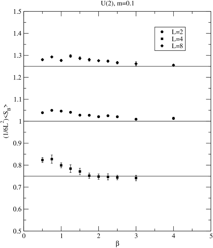
Figure 1: $\frac{\beta}{6L^{2}}<S_{B}>$ for $U(2)$ at $m=0.1$

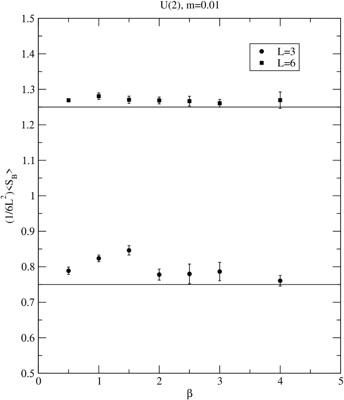
Figure 2: $\frac{\beta}{6L^{2}}<S_{B}>$ for $U(2)$ at $m=0.01$

where $N_{g}=4$ is the number of generators of $U(2)$. Figure 1. shows a plot of $\frac{\beta}{6L^{2}}<S_{B}>$ for a range of couplings $\beta$ and three different lattice sizes using a mass $m=0.1$. The bold lines shows the analytic prediction based on supersymmetry (for clarity we have added multiples of $-0.25$ to the curves and lines to split up the data from different lattice sizes) While there are clearly deviations of order 4-5% at small coupling these appear to disappear at large $\beta$ in line with our expectations. Figure 2. shows equivalent data for $L=3,6$ at the smaller gluino mass $m=0.01$. Again the horizontal lines show the analytic result expected from supersymmetry. In this case the deviations for the small lattice appear larger at small coupling but nevertheless appear to converge toward the theoretical expectation on the basis of supersymmetry as $\beta$ is increased. The larger lattice $L=6$ data are even better. We have also examined other Ward identities corresponding to the local operator choices

$$O = O_{1}(x)=\overline{\eta}(x)[\phi(x),\overline{\phi}(x)]$$

$$O = O_{2}(x)=\overline{\chi}_{\mu\nu}F_{\mu\nu}$$

$$O = O_{3}(x)=\overline{\psi}_{\mu}(x)D^{+}_{\mu}\overline{\phi}(x)$$ (45)

After $Q$-variation we find

$$QO_{1} = [\phi,\overline{\phi}]^{2}-\overline{\eta}[\phi,\eta]$$

$$QO_{2} = F^{\dagger}_{\mu\nu}(x)F_{\mu\nu}(x)-\overline{\chi}_{\mu\nu}D^{+}_{\left[\mu\right.}\psi_{\left.\nu\right]}$$

$$QO_{3} = -D^{+}_{\mu}\phi D^{+}_{\mu}\overline{\phi}-\overline{\psi}_{\mu}D^{+}_{\mu}\eta-\overline{\psi}_{\mu}[\overline{\psi}_{\mu},\phi]$$ (46)

The results for expectation values of these $Q$-variations for $\beta=4.0$ and $m=0.01$ are displayed in tables 1. and 2. corresponding to lattice sizes $L=3$ and $L=6$ respectively (we denote the bosonic contribution to the Ward identity by $B$ and the fermionic one by $F$).

$O$	$B$	$Re(F)$	$Im(F)$
$O_{1}$	$0.88(7)$	$-0.86(6)$	$-0.0003(5)$
$O_{2}$	$0.285(16)$	$-0.297(16)$	$-0.0009(28)$
$O_{3}$	$0.90(45)$	$-0.986(4)$	$0.0035(39)$

Table 1: Ward identities for $U(2)$ and $\beta=4.0$,$L=3$

$O$	$B$	$Re(F)$	$Im(F)$
$O_{1}$	$0.38(8)$	$-0.43(10)$	$-0.0008(15)$
$O_{2}$	$0.409(22)$	$-0.386(25)$	$-0.0006(7)$
$O_{3}$	$1.22(49)$	$-0.995(1)$	$-0.0003(20)$

Table 2: Ward identities for $U(2)$ and $\beta=4.0$,$L=6$

Notice that the imaginary part of the fermionic correlator is always small and statistically consistent with zero. Within the statistical errors the bosonic and fermionic contributions do add to zero confirming the presence of the $Q$-symmetry in the quantum lattice theory for this coupling.

The apparent breaking of supersymmetry at small $\beta$ appears to be correlated to the symmetry properties of the lattice fermion operator $M(U,\phi)$. In the continuum this operator is complex antisymmetric and hence its determinant can be written as the square of a Pfaffian. This is true for both $SU(2)$ and $U(2)$ theories (the $U(1)$ or trace mode of the scalars and gauge field disappear from the fermion operator for all couplings rendering both continuum theories equivalent in this respect).

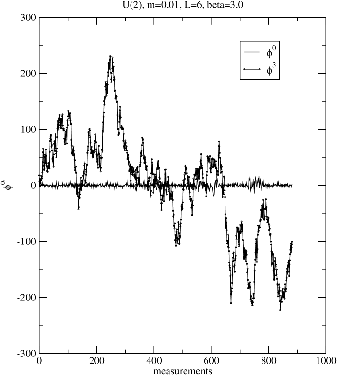
Figure 3: Monte Carlo evolution of trace and traceless components of scalars

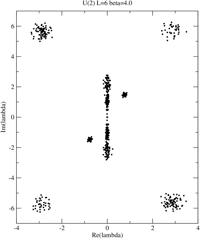
Figure 4: Eigenvalue spectrum for $U(2)$ theory at $\beta=4.0$

The antisymmetric condition is very important also in the lattice theory because in this case we have argued that the real and imaginary components of the fermion decouple - a necessary condition for existence of a Pfaffian and the truncation of the theory to the real line. If the matrix is not antisymmetric this factorization cannot be achieved and supersymmetry must necessarily be broken. In the case of $SU(2)$ it is not hard to see that the matrix is indeed antisymmetric and we exploit this fact later when we examine the phase of the Pfaffian for the $SU(2)$ system. This property is not shared by the $U(2)$ model in general though since the trace degrees of freedom of the gauge link do not decouple for finite $\beta$. Approximate decoupling will now occur in the region of large coupling $\beta$ where the approximation $U_{\mu}(x)=1+A_{\mu}(x)+\cdots$ becomes accurate. By examining the fourth root of the plaquette we learn that $|A_{\mu}|\sim 0.05$ for $\beta=3.0$. Hence corrections to this approximation will be less than one percent if $\beta>3$ consistent with the restoration of supersymmetry we see in the large $\beta$ regime. This decoupling can be seen explicitly in figure 3. which shows the Monte Carlo evolution of the scalar field for $\beta=3.0$, $L=6$ and $m=0.01$ in the $U(2)$ theory. Two modes are shown corresponding to $\phi^{3}$ (the trace mode) and $\phi^{0}$ a traceless mode. The trace mode $\phi^{3}$ behaves as a quasi massless degree of freedom undergoing large fluctuations regulated only by the imposed IR cut-off of $m=0.01$ while the traceless degrees of freedom fluctuate independently over a scale two orders of magnitude smaller. The spectrum of a typical equilibrated configuration for $\beta=4.0$ on a lattice of size $L=6$ is shown in figure 4. Much of the spectrum is concentrated close to the imaginary axis and is indicative of light continuum-like states. Notice the approximate pairing of eigenvalues $(\lambda,-\lambda)$ related to the approximate antisymmetry of the fermion operator at this large coupling. There are in addition “islands” of additional states at large eigenvalue which we conjecture are related to the large fluctuations of the nonzero trace modes of the scalars. These don’t appear to have any continuum interpretation.

6 Phase quenched SU(2) model

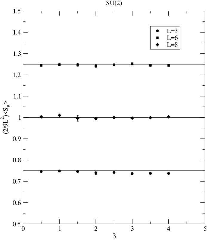
Figure 5: $\frac{2\beta}{9L^{2}}<S_{B}>$ for $SU(2)$

Since the $SU(2)$ theory contains no exact zero modes we have been able to simulate the model at exactly zero gluino mass. Figure 5. shows a plot of the mean bosonic action normalized to unity as a function of $\beta=0.5\to 4.0$ for $L=3,6,8$ for the $SU(2)$ theory. In contrast with the $U(2)$ lattice theory the scalar supersymmetry appears to be good here down to small coupling $\beta$. As we have remarked we conjecture that this is related to the presence of an exact antisymmetry of $M$ in the $SU(2)$ case. Clearly the Yukawas possess this property. What is non trivial is that this is also true of the gauged lattice Kähler-Dirac term. In general this term is antihermitian but in the case of $SU(2)$ it is also real. This follows from the special property of the Pauli matrices

$$e^{\mu_{i}\sigma_{i}}=\cos{\left|\mu\right|}I+\frac{\sin{\left|\mu\right|}}{\left|\mu\right|}\mu_{i}\sigma_{i}$$ (47)

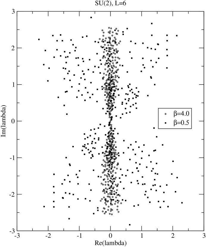
Figure 6: Eigenvalue spectrum for $SU(2)$ theory at $L=6$

Using this representation it is easy to show that $V_{\mu}^{ab}(x)$ is real. Figure 6. shows a plot of the eigenvalues of the $SU(2)$ theory for $L=6$ at both $\beta=0.5$ and $\beta=4.0$ in which the exact pairing of eigenvalues is manifest. Notice that as $\beta$ increases the real parts of these eigenvalues decrease. In the limit we expect the eigenvalues to lie along the imaginary axis yielding a real, positive definite determinant as for the continuum theory. We have additionally measured the same local Ward identities as for $U(2)$ with the results listed in tables 3. and 4. Here, the data is taken from runs with $L=6$ and two different values of the coupling $\beta=0.5$ and $\beta=4.0$.

$O$	$B$	$Re(F)$	$Im(F)$
$O_{1}$	$4.70(20)$	$-4.72(04)$	$-0.04(04)$
$O_{2}$	$1.95(07)$	$-2.02(02)$	$0.014(14)$
$O_{3}$	$5.76(15)$	$-5.74(05)$	$-0.043(35)$

Table 3: Ward identities for $SU(2)$ and $\beta=0.5$,$L=6$

$O$	$B$	$Re(F)$	$Im(F)$
$O_{1}$	$0.167(10)$	$-0.195(8)$	$-0.007(07)$
$O_{2}$	$0.344(10)$	$-0.346(1)$	$-0.0007(8)$
$O_{3}$	$0.759(21)$	$-0.739(4)$	$0.0012(17)$

Table 4: Ward identities for $SU(2)$ and $\beta=4.0$,$L=6$

Again for both small and large coupling these local Ward identities appear to be satisfied to within statistical error.

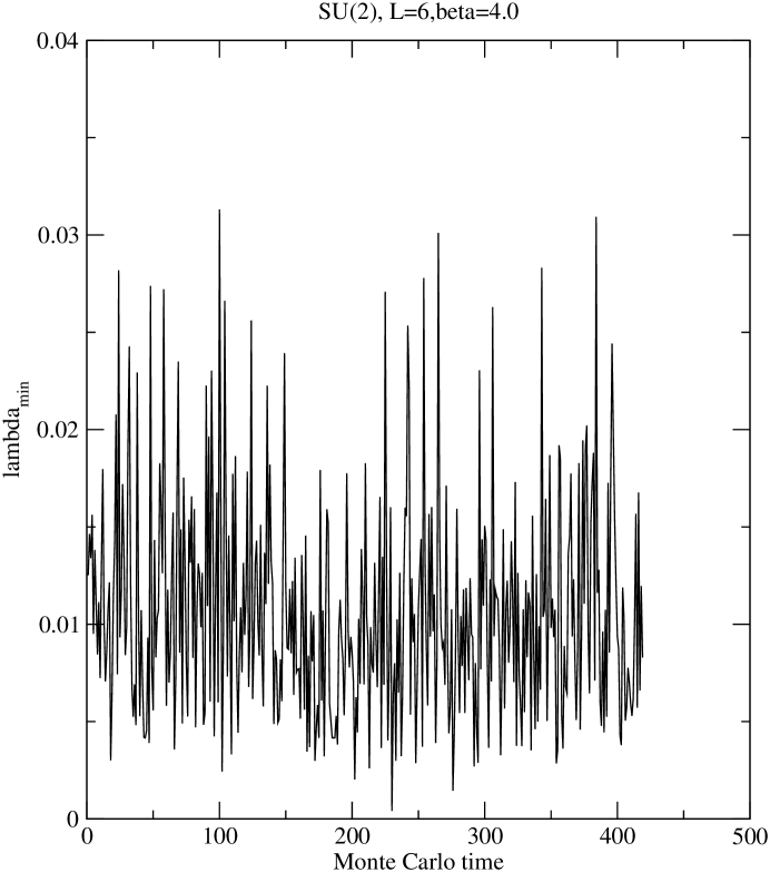
Figure 7: Minimum eigenvalue for $SU(2)$ theory at $L=6$

Since the simulations of the $SU(2)$ are carried out at zero mass we have a priori no lower bound on the eigenvalue spectrum and so we monitor the smallest eigenvalue continuously to ensure it lies within the limits required by our minimax approximation to the inverse fourth root of the fermion operator. A typical plot of the Monte Carlo evolution of $|\lambda_{\rm min}|$ is shown in figure 7. We observe that the magnitude of this smallest eigenvalue decreases with increasing $\beta$ and $L$ but we see no evidence for an exact zero mode as would be expected for a supersymmetric theory whose flat directions survive quantum corrections. We will return to this issue when we discuss the quantum moduli space.

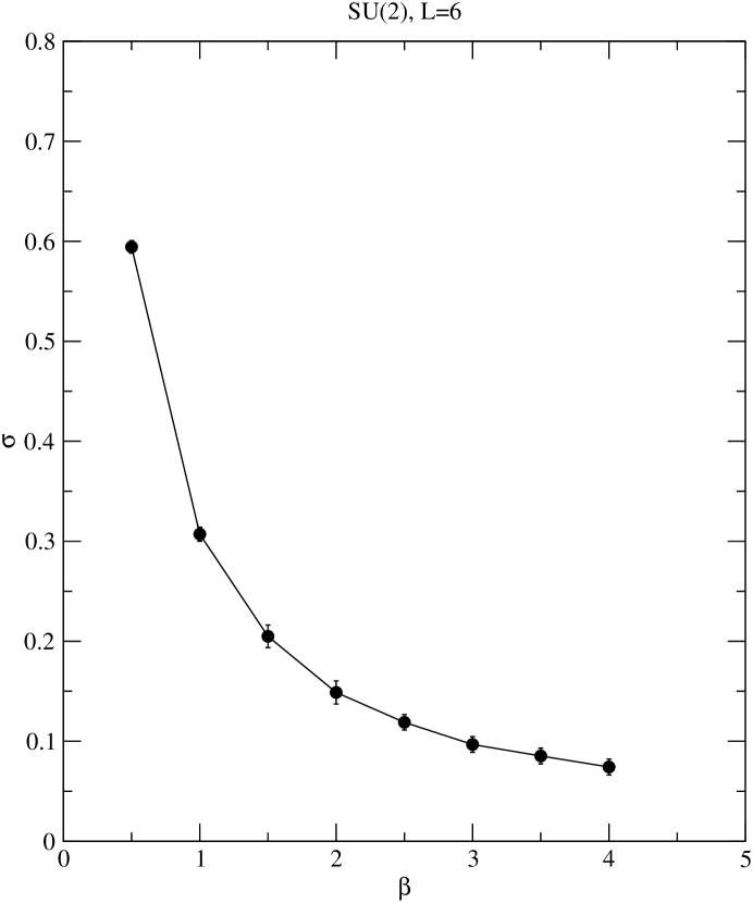
Figure 8: String tension for $SU(2)$ and $L=6$

Since we employ periodic boundary conditions the partition function we simulate yields the Witten index of the theory and is explicitly independent of coupling constant (recall that $\frac{\partial lnZ}{\partial\beta}=<S>=0$). This in turn implies that there can be no thermodynamic singularity for finite $\beta$ and we expect the theory exists in a single phase. Figure 8. confirms this expectation by plotting the string tension as estimated from the $2\times 2$ Creutz ratio as a function of $\beta$ for a lattice of size $L=6$. The string tension appears to be non-zero and smoothly varying over this range of coupling.

We have also examined a couple of correlation functions which give us direct access to the low-lying mass states of the theory. The simplest $SO(1,1)$ and gauge invariant bosonic correlator takes the form

$$G_{B}(t)=\sum_{x,x^{\prime}}<\phi^{a}(x,t)\overline{\phi}^{a}(x,t)\phi^{b}(x^{\prime},0)\overline{\phi}^{b}(x^{\prime},0)>$$ (48)

and the sum over spatial sites $x,x^{\prime}$ projects to the zero momentum sector. We have also examined a fermionic correlator of the form

$$G_{F}(t)=\sum_{x,x^{\prime}}<\overline{\eta}^{a}(x,t)\phi^{a}(x,t)\eta^{b}(x^{\prime},0)C^{b}(x^{\prime},0)>$$ (49)

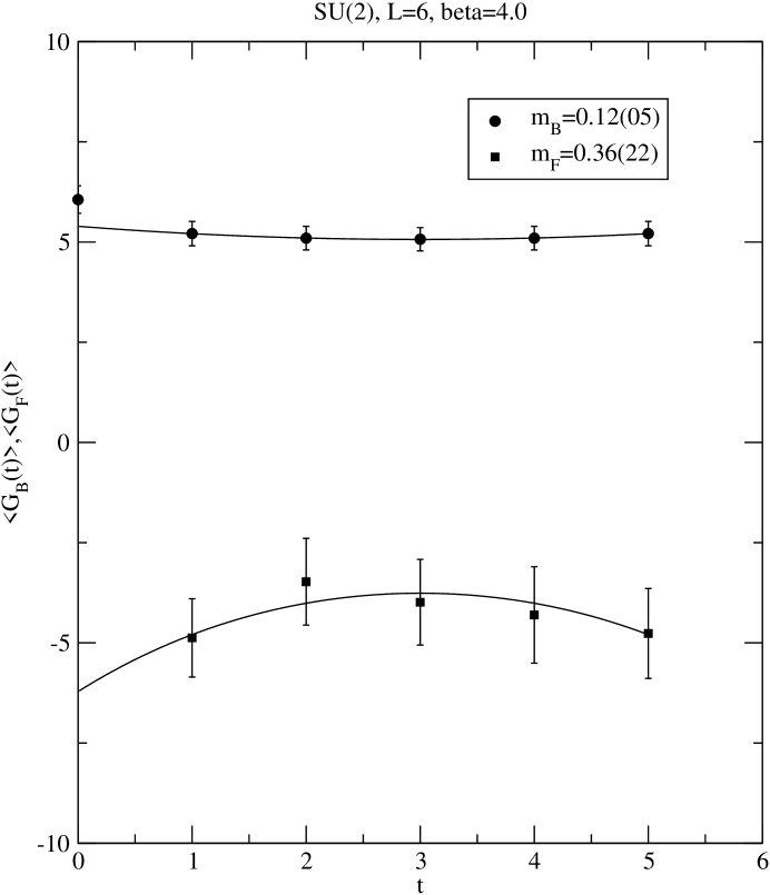
Figure 9: Bosonic and fermionic correlators in $SU(2)$ for $L=6$ and $\beta=3.0$

where $C=[\phi,\overline{\phi}]$. These functions are shown in figure 9. together with fits to hyperbolic cosines. As a consequence of supersymmetry we expect that the lowest lying bosonic and fermionic states should have the same mass. Within statistical errors this is true (and indeed this state is rather light). However the errors on the fermion are large and the current data is really inadequate to decide this question. Of course it is also not clear we have the correct interpolating operator for the lightest fermion state – further investigations of these issues are underway.

7 Reality of the fermionic effective action

Up to this point we have neglected a possible phase associated with the Pfaffian induced by integration over the fermion fields. As we have seen the truncation to the real line in general breaks the supersymmetry in the $U(2)$ model so we will concentrate on the $SU(2)$ case where the fermion operator is an antisymmetric matrix and a Pfaffian can be unambiguously defined. As usual we can always compensate for neglecting this phase in the Monte Carlo simulation by re-weighting all observables by the phase factor according to the simple rule

$$<O>=\frac{<Oe^{i\alpha(U,\phi)}>_{\rm\alpha=0}}{<e^{i\alpha(U,\phi)}>_{\rm\alpha=0}}$$ (50)

We thus have computed the Pfaffian as one of our observables allowing us to carry out this re-weighting procedure when computing expectation values. The Pfaffian computation is carried out by using a variant of Gaussian elimination with full pivoting to transform the $2n\times 2n$ dimensional antisymmetric matrix $M$ into the canonical form

$$\left(\begin{array}[]{ccccc}0&\lambda_{1}&0&0&\ldots\\ -\lambda_{1}&0&0&0&\ldots\\ 0&0&0&\lambda_{2}&\ldots\\ 0&0&-\lambda_{2}&0&\ldots\\ 0&0&0&0&\ldots\\ \end{array}\right)$$ (51)

Then

$${\rm Pf}(M)=\prod_{i=1}^{n}\lambda_{i}$$ (52)

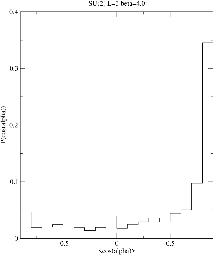
Figure 10: $P(\cos{\alpha})$ vs $\cos{\alpha}$ for $L=3$ $\beta=4.0$

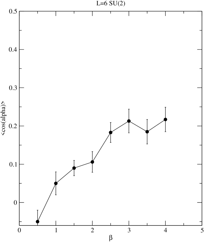
Figure 11: $<\cos{\alpha}>$ for $L=3$

Consider first the phase itself. Figure 10. shows a plot of the distribution of $\cos{\alpha}$ for $L=3$ and $\beta=4.0$. A strong peak close to $\alpha=0$ is manifest. This peak strengthens with increasing $\beta$ as the scalars (which are responsible for a non-zero phase) are driven closer to zero. Figure 11. shows a plot of $\cos{\alpha}$ vs $\beta$ for $L=6$ ($<\sin{\alpha}>$ is small and always statistically consistent with zero). We see that it increases from values close to zero to attain

$$<\cos{\alpha}>\sim 0.2\qquad\beta=4.0$$ (53)

Hence, in the range of coupling we have simulated, it clearly fluctuates strongly from the naive value of unity used in generating the phase quenched ensemble. In light of this we have re-examined the Ward identities now weighted with this phase factor. Table 5. shows the mean re-weighted bosonic action together with the phase quenched value for $L=3$ and all $\beta$ (note that these numbers are not normalized to unity as in the earlier plots). While re-weighting typically amplifies the estimated error it does not appear to change the mean value for this observable at least within the statistical errors.

$\beta$	$S_{B}$	${\rm Reweighted}\;S_{B}$
$0.5$	$40.35(19)$	$39.80(95)$
$1.0$	$40.45(18)$	$40.42(117)$
$2.0$	$40.11(32)$	$40.80(130)$
$2.5$	$40.16(32)$	$40.62(130)$
$3.0$	$39.74(25)$	$40.11(140)$
$3.5$	$39.99(30)$	$40.58(200)$
$4.0$	$39.73(30)$	$39.66(220)$

Table 5: Ward identities for $SU(2)$ and $\beta=4.0$,$L=6$

This conclusion is strengthened by examining other re-weighted Ward identities corresponding to the set of operators $O_{1}$, $O_{2}$ and $O_{3}$ given earlier. Tables 6. and 7. compare the naive (phase quenched) expectation values with their re-weighted values for lattice size $L=6$ and $\beta=0.5$ and $\beta=4.0$. Again, there is no evidence that the central values change within the (admittedly large) statistical errors.

$O$	$B$	$Re(F)$	Reweighted $B$	Reweighted $Re(F)$
$O_{1}$	$4.70(20)$	$-4.72(03)$	$6.46(210)$	$-5.04(100)$
$O_{2}$	$1.95(07)$	$-2.02(02)$	$2.14(100)$	$-2.01(50)$
$O_{3}$	$5.76(15)$	$-5.74(02)$	$5.74(200)$	$-5.25(200)$

Table 6: Naive vs reweighted Ward identities for $SU(2)$ and $\beta=0.5$,$L=6$

$O$	$B$	$Re(F)$	Reweighted $B$	Reweighted $Re(F)$
$O_{1}$	$0.167(10)$	$-0.195(7)$	$0.159(40)$	$-0.137(50)$
$O_{2}$	$0.344(10)$	$-0.346(1)$	$0.356(60)$	$-0.348(50)$
$O_{3}$	$0.759(21)$	$-0.739(4)$	$0.717(110)$	$-0.733(120)$

Table 7: Naive vs reweighted Ward identities for $SU(2)$ and $\beta=4.0$,$L=6$

Taken at face value this apparent weak dependence of the expectation values on reweighting seems to indicate that the phase fluctuates approximately independently of the other observables leading to an, at least approximate, factorization in the reweighted observable

$$<O>_{\rm full}=\frac{<Oe^{i\alpha}>_{\alpha=0}}{<e^{i\alpha}>_{\alpha=0}}\sim\frac{<O>_{\alpha=0}<e^{i\alpha}>_{\alpha=0}}{<e^{i\alpha}>_{\alpha=0}}=<O>_{\alpha=0}$$ (54)

As a practical matter this means that expectation values obtained within the phase quenched approximation may be quite reliable in spite of the large phase fluctuations.

8 Quantum moduli space

Finally we turn to an important issue concerning the two scalar fields that appear in this theory. The classical vacua allow for any set of scalars which are constant over the lattice and satisfy

$$[\phi,\overline{\phi}]=0$$ (55)

In the case of $SU(2)$ and using the parameterization $\phi=\phi_{1}+i\phi_{2}$ we find vacuum states of the form

$$\phi_{1}=(A,0,0)\qquad\phi_{2}=(B,0,0)$$ (56)

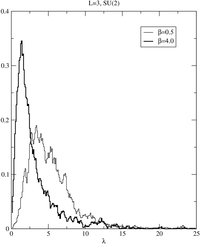
Figure 12: Distribution of eigenvalues of $\phi_{1}$ for $SU(2)$, $L=6$

together with global $SU(2)$ rotations of this configuration. Thus we have a classical vacuum state for any value of $A$ and $B$. This space of vacuum solutions is referred to as the moduli space of the theory. The presence of such a non-trivial moduli space corresponds to the existence of flat directions in the theory. This is problematic in the quantum theory as integration over such flat directions may induce IR divergences. However we find that this is not the case in practice – the quantum ground state appears to be unique and the flat directions are lifted (except for the trivial $U(1)$ factor associated with trace part of $U(2)$). This can be seen from the distribution of eigenvalues of the scalars averaged over the lattice. Figure 12. shows a plot of this distribution for the $SU(2)$ theory on a $L=3$ lattice both for $\beta=0.5$ and $\beta=4.0$. The distribution is symmetric about the origin so we show only the positive values here. Both for small and large coupling the distribution possesses a well defined peak with a tail extending out to large eigenvalue. Notice that the peak moves to smaller values as $\beta$ increases in line with the observed suppression of scalar field fluctuations with increasing coupling. The data indicates that the partition function at least exists and most likely at least some of the lower moments of the scalar field. This result is reminiscent of similar results obtained for zero dimensional supersymmetric Yang-Mills integrals [35].

9 Conclusions

In this paper we have presented initial results from a full simulation of the ${\cal N}=2$ super Yang-Mills theory in two dimensions. The lattice action we employ was derived in [1] and follows from a reformulation of the theory in terms of twisted fields. It is invariant under a global $SO(1,1)$ symmetry and $U(N)$ lattice gauge transformations and exhibits, at least in its complex form, an exact scalar supersymmetry. We show results for both $U(2)$ and $SU(2)$ theories for a range of lattice size $L$ and coupling $\beta$. To check for supersymmetry we have examined a number of Ward identities.

In the case of $U(2)$ the supersymmetry appears to be only exact at large $\beta$. At small $\beta$ the fermion operator is not antisymmetric, its Pfaffian is not even defined and the truncation of the complexified theory to the real line appears to break supersymmetry. However, the theory does not seem to need any fine tuning to regain supersymmetry for large coupling $\beta$ and hence in the continuum limit.

In the case of $SU(2)$ the lattice gauged Kähler-Dirac operator is real and antisymmetric and supersymmetry is manifest for all couplings - we see no statistically significant violation of any Ward identities at the 1% level for any coupling or lattice size. We conjecture that the key property which allows the supersymmetry to be realized is the antisymmetric property of the fermion operator. Since the latter is always antihermitian this in turn boils down to a reality property on the gauged Kähler-Dirac operator. At first glance it appears that $SU(2)$ is rather special in this regard. However, reality of the $SU(N)$ theories will be guaranteed for all $N$ if instead of using the $N\times N$ basis for the generators we employ the basis constructed from the structure constants themselves $T^{a}_{bc}=f_{abc}$. Such a choice yields the same naive continuum limit but guarantees that the gauged Kähler-Dirac action is real and antisymmetric. We conjecture that such models will resemble $SU(2)$ and exhibit an exact scalar supersymmetry at the quantum level.

In the case of $SU(2)$ we have also examined the validity of the phase quenched approximation used in our simulations. The phase appears to approach zero in the large $\beta$ continuum limit as naively expected. Remarkably, re-weighting observables with the phase does not appear to have a strong influence on expectation values even for small $\beta$ at least in the case of observables corresponding to Ward identities. We also show results on the distribution of the eigenvalues of the scalar fields. This distribution possess a well-defined peak which narrows and moves to smaller values as $\beta$ increases. This structure is similar to the case of zero dimensional SUSY Yang-Mills and indicate that the classical vacua are lifted via quantum effects.

To summarize, our initial numerical investigations of twisted formulations of lattice super Yang-Mills theories are quite positive – it appears that full dynamical simulations of these theories are possible with rather moderate computational resources (the work presented here was obtained with $O(300)$ single CPU days on a P3 cluster). These preliminary results provide evidence that supersymmetry is indeed realized at the quantum level and have already allowed us to check certain qualitative features of the theory – for example, our data support the lifting of the classical vacua and finiteness of the partition function. They also support a single phase picture for this theory. It would be nice to extend these calculations to larger lattices to be able to get more reliable results for the low-lying spectrum which could be compared to the SDLCQ results reported in [36] and to the dimensionally reduced quantum mechanics case [37]. It is important also to examine Ward identities corresponding to other elements of the twisted supersymmetry to see whether indeed the other supersymmetries are realized without fine tuning in the continuum limit. Results from these investigations will be published elsewhere [38].

It should be stressed that low dimensional super Yang-Mills theories are of great interest because of their conjectured connections to various types of (super)gravity theory. They are a place where lattice simulations could potentially play an important role since high precision exact dynamical simulations are possible on large lattices. In principle, the strongest connections to gravitational systems are exhibited for theories with sixteen supercharges rather than the four supercharge case considered here. However, dimensional reduction of the ${\cal N}=D=4$ lattice action constructed in [24] would yield $Q$-exact actions for these systems whose fermion content could be represented using Kähler-Dirac fields. Notice that although the Kähler-Dirac action is related to the usual staggered fermion action there is no “fourth root” problem with these theories since the fermion degeneracy associated with these lattice actions precisely accounts for the number of physical fermions required by the extended supersymmetry.