Calorons and monopoles from smeared $SU(2)$ lattice fields at non-zero temperature

Abstract

In equilibrium, at finite temperature below and above the deconfining phase transition, we have generated lattice $SU(2)$ gauge fields and have exposed them to smearing in order to investigate the emerging clusters of topological charge. Analysing in addition the monopole clusters according to the maximally Abelian gauge, we have been able to characterize part of the topological clusters to correspond either to non-static calorons or static dyons in the context of Kraan-van Baal caloron solutions with non-trivial holonomy. We show that the relative abundance of these calorons and dyons is changing with temperature and offer an interpretation as dissociation of calorons into dyons with increasing temperature. The profile of the Polyakov loop inside the topological clusters and the (model-dependent) accumulated topological cluster charges support this interpretation. Above the deconfining phase transition light dyons (according to Kraan-van Baal caloron solutions with almost trivial holonomy) become the most abundant topological objects. They are presumably responsible for the magnetic confinement in the deconfined phase.

I Introduction

In our previous work IMMPV05 we have started an investigation of topological objects that appear in the course of smearing smearing of equilibrium lattice fields. These were generated at finite temperature in the confining phase of SU(2) lattice gauge theory. The main idea was to analyze the monopole content of these objects, still far from being classical solutions, according to the maximally Abelian gauge (MAG) in order to classify them as related to non-static calorons or static dyons. Such a classification would be natural in the context of Kraan-van Baal (KvB) caloron solutions with non-trivial holonomy KvB-1 ; KvB-2 ; LeeLu . In the present paper, using some additional techniques, we take up this problem again, now for a couple of temperatures below and above $T_{\rm dec}$.

Before pointing out the new tools for this analysis, we should briefly recall the general view and the terminology used, that originate from the classical KvB solutions KvB-1 ; KvB-2 . We will do this for the simplest case, the $SU(2)$ gauge theory. In this case, at finite temperature, the classical carriers of one unit of topological charge are selfdual or antiselfdual objects (periodic caloron solutions) which consist of two monopole “constituents”. In the limit of small inter-monopole distances they form a single, non-static caloron, whereas at large distances they dissociate into a pair of separate static lumps of action and topological density (static Bogomolnyi-Prasad-Sommerfield (BPS) monopoles BPS or “dyons”). In the latter case the action $8\pi^{2}/g^{2}$ (or one unit of topological charge) is shared among the constituents according to the holonomy of the gauge field, in the ratio $~{}\overline{\omega}/\omega$,  where $~{}\overline{\omega}=1/2-\omega$. The asymptotic value of the Polyakov loop

$$L_{\infty} = \lim_{|\vec{x}|\to\infty}L(\vec{x})$$ (1)

$$= \lim_{|\vec{x}|\to\infty}\frac{1}{2}~{}\mathrm{tr}~{}{\bf P}~{}\exp\left(i\int_{0}^{b=1/T}A_{4}(\vec{x},t)~{}dt\right)$$

$$= \cos(2\pi\omega),~{}~{}0\leq\omega\leq 1/2\,,$$

determines the holonomy parameter $\omega$ and its complement $\overline{\omega}$.

Each physical phase can be thought as a medium creating a certain $L_{\infty}$ as boundary condition for the calorons. For example, maximally non-trivial asymptotic holonomy, $~{}L_{\infty}=0~{}$ or $~{}\overline{\omega}=\omega=1/4$, forces the constituents to carry equal topological charge $~{}\pm 1/2$. With the holonomy becoming more and more trivial with increasing temperature, $~{}L_{\infty}\to\pm 1~{}$, the constituents become imbalanced. On the other hand, the constituents are distinguished by the local behavior of the Polyakov loop $~{}L({\vec{x}})\approx\pm 1$ close to their positions. This is the characteristic signature, irrespectively whether the action forms two separated lumps or a single lump, the latter one with unit topological charge.

Viewed by Abelian monopoles appearing in the MAG, static dyons are represented by monopoles temporally wrapping around the lattice, whereas single non-static calorons are localized in time and have monopole loops of finite extent running close to the center. This feature of calorons in the MAG has been pointed out first by Brower et al. Brower . This was our guiding hypothesis already in Ref. IMMPV05 . In Fig. 1 we show a classical caloron solution in the two limiting cases together with the corresponding MAG monopole content.

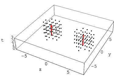
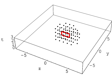
Figure 1: (color online) Left: two static dyons accompanied by two static monopoles; right: a single caloron accompanied by a monopole loop. The classical $SU(2)$ configurations have been generated on a $16^{3}\times 4$ lattice and then Abelian-projected. In the $(z,y,t)$ lattice at $x=0$ we show the sites with action density $s>s_{\rm max}/5$ (left, for dyons) and $s>s_{\rm max}/40$ (right, for calorons) together with the emerging monopole trajectories.

In Ref. recombination we have seen such static monopoles also in the Polyakov gauge, regularly accompanying static, i.e. dissociated caloron configurations while being rarely found in non-static calorons.

According to the scenario to be outlined in Sec. II we expect to observe below $T_{\rm dec}$ both dissociated and non-dissociated clusters of topological charge $\pm\frac{1}{2}$ and $\pm 1$, respectively, in some mixture. Above $T_{\rm dec}$ only clusters with charge $\pm 1$ should remain, with a density decreasing with increasing temperature. That means that we are expecting to see calorons with trivial holonomy actually dominating the topological charge above $T_{\rm dec}$.

The topological structure in the deconfined phase is partly also a question concerning the capability of the smearing method applied in this paper. Whereas the topological structure is known to be preserved under smearing in the confined phase, experience shows that under comparable smearing conditions the topology is rapidly wiped out in the deconfined phase. Therefore, in order to escape these bad prospects, we have to modify the smearing conditions in the deconfined phase.

We point out in Sec. II that there are fermionic methods to determine the topological density but, in order to detect a semiclassical structure, certain UV smearing techniques have to be applied as well. Our analogous method applied for the same purpose is a combination of gluonic measurements of the most naive topological charge density combined with the monopole localization in the maximally Abelian gauge. Both are applied to APE smeared configurations. In a very recent paper it has been demonstrated, by comparison of smeared and cooled configurations with the original equilibrium configurations, that the spectrum of a chirally improved Dirac operator remains practically unaltered GattringerIlgenfritzSolbrig meaning that the infrared structure “seen by the low-lying chiral fermion modes” in equilibrium, is conserved under controlled cooling or moderate smearing.

Since for our purpose the correlation with Abelian monopoles is of crucial importance, the technical improvements (compared to Ref. IMMPV05 ) in the present paper are concerning the methods detecting the monopole structure. This applies both to gauge fixing and to the analysis of separable monopole loops. We have now fixed the MAG by the more advanced technique of simulated annealing simulated_annealing . This method is known to lead, in comparison with the overrelaxation method, to higher maxima of the gauge functional and to a minimal monopole content. Analogously to the preceding paper, the detection of monopole trajectories is used here to identify clusters of the topological charge density resembling the two extreme appearances of KvB calorons. Unlike the previous paper, we are now actually exploring the full monopole content of individual topological objects, not only looking for intersections of time-like monopole currents with the topological charge clusters IMMPV05 . We are taking the precise type of monopole clusters into account.

Last but not least, we use now a larger lattice (with size $24^{3}\times 6$) and a certain set of different $\beta$-values. Three values, $\beta=2.2,~{}2.3,~{}2.4$, belong to the confined phase while the remaining two values of $\beta=2.5,~{}2.6$, represent the deconfined phase. This will allow us to get information about the temperature dependence of the caloron/dyon composition that was left open in the previous investiagtions.

In Sec. II we will outline the general physical picture behind the present investigation. In Sec. III we will briefly explain the set of our runs and in particular the conditions for the smearing procedure. In Sec. IV we shall describe the local influence of monopoles altering the distribution of the Polyakov loop. This part is interesting by its own and is not related to the following cluster analysis. In Sec. V we will describe the results of the analysis of topological clusters. The classification with the help of monopoles will be of use here. We draw our conclusions in Sec. VI.

II The physical picture

The one-loop calculation of the caloron amplitude Diakonov has shown that below some temperature calorons may become instable with respect to the separation into their constituents. It would be attractive to identify this temperature with the deconfinement temperature because, in a dilute gas calculation, it has been shown that at this temperature trivial holonomy $L_{\infty}\approx 1$ turns from a minimum of the free energy $P$ (as a function of $L_{\infty}$) into a maximum. The global view of the function $P(L_{\infty})$ is, however, beyond the capability of the dilute caloron gas approximation. In a schematic dyon gas model, Diakonov Diakonov_review has demonstrated how the stability of $L_{\infty}=0$ (being the minimum of $P$) could eventually be achieved.

All this taken together leads to a simplified picture that describes the essence of the transition to confinement as the dissociation of tightly bound calorons (with trivial asymptotic holonomy) into dissociated ones with nontrivial holonomy and discernible dyonic constituentis. This cannot be the full truth, however. As we know from Refs. Brower ; recombination , at low temperature calorons, even of nontrivial holonomy, are likely to appear as single lumps of action that nonetheless are different from the well-known instanton solutions because of the nontrivial holonomy boundary conditions they must satify in the confining medium.

Therefore we expect to observe in a study at different temperatures the constituents becoming manifest inside dissociated calorons more abundantly approaching the deconfining transition from below. Whereas the topological susceptibility is temperature independent throughout the confined phase, the relative abundance of static objects with an appreciable fractional topological charge (close to $\pm\frac{1}{2}$) should increase towards the phase transition temperature compared to the abundance of non-static calorons.

We have announced in the Introduction that we have used four-dimensional smearing for this investigation. There is an alternative way to locate calorons and their constituents, respectively. It is based on the localization behavior of the zero modes and the near-zero modes of the Dirac operator GPGAPvB ; CKvB . A jumping behavior of the zero mode in charge $Q=\pm 1$ configurations can be observed under the influence of changing boundary conditions, deliberately imposed on the fermion field. This is very reminiscent to what is familiar from the case of an exact caloron background field. Interpolating with an appropriate phase factor between periodic boundary conditions and antiperiodic ones, the zero mode may jump from one constituent to another.

For various classical solutions extracted on the lattice by the cooling method this has been established for $SU(2)$ WeWithStanislav as well as for $SU(3)$ WeWithPeschka . For equilibrium lattice gauge fields selected to possess unit topological charge, in the $SU(3)$ and $SU(2)$ cases a similar “jumping” of lowest-lying modes of a chirally improved lattice Dirac operator was reported by Gattringer and coauthors GattringerSchaefer ; GattringerPullirsch ; GattringerSolbrig . Of course, $Q=\pm 1$ equilibrium configurations generically contain more clusters and spatial fluctuations of topological charge than the single zero-mode is able to detect. Such configurations differ from a pure (anti-)caloron even in the deconfined phase. It has been verified Lattice03 , that the single zero mode is always attracted to positions that are maxima of the topological density inside extended topological clusters. This check has required a very well-tuned smearing and has used a topological charge operator defined in terms of the naive twisted plaquette. However, there were more clusters and cluster maxima going undetected by the single zero mode. In our previous IMMPV05 and in the present paper, the diagnostic role is shifted to the MAG monopoles. Note that these are not limited in number or to a particular chirality as the zero modes are.

With a chirally perfect or improved Dirac operator at hand (that satisfies the Ginsparg-Wilson equation), there is a definition overtopdefinition of the topological charge density which is equivalent, in the continuum limit, to the gluonic definition. It may supersede a gluonic definition at finite lattice spacing. This density also exposes a clustering pattern Koma ; Weinberg ; Nicosia strongly dependent on ultraviolet filtering, usually implemented by a cutoff (in eigenvalues) of the contributing eigenmodes. The non-filtered density, in contrast, contains fluctuations of all scales and cannot be related to a semiclassical model. An analysis of calorons and dyons using these tools along the ideas of the present paper is left for the future.

In Ref. InstantonQuarks it has been attempted to construct single-caloron and multi-caloron solutions at lower temperature starting from high temperature ones. It was characteristic that all classical constituents were delocalized to a scale set exclusively by the periodic 4-volume, in contrast to the (jumping) zero modes seen also in zero temperature equilibrium configuration background configurations which are highly localized due to quantum fluctuations of the gauge field. This limits our expectations to find, in the limit of vanishing temperature, a semiclassical structure that would reveal the elusive “instanton quarks” in separation.

Using the new procedures under wider physical conditions at finite temperatures, similar to Ref. IMMPV05 we will observe both non-static calorons and static dyons. In the confined phase the relative population of isolated dyons will be seen growing with increasing temperature. This will be interpreted as progressive dissociation (dipole splitting) of calorons into dyons in the confined phase. This is the main result of our paper directly related to the KvB caloron picture and confirming the simplified picture described above.

Unexpectedly from the point of view of the scenario outlined above, in the deconfined phase nondissociated calorons are rare objects, even though charge $Q=\pm 1$ configurations are still observed after a well-tuned amount of smearing. According to the different asymptotic holonomy (changing away from vanishing Polyakov loop toward $L_{\infty}\neq 0$) one would expect an extreme asymmetry among the constituent dyons if they appear at all. One type of dyons should be small in size and heavy in action with a peak of the Polyakov loop of opposite sign with respect to $L_{\infty}$, and another type of dyons large in size and light in action with a peak of the Polyakov loop of equal sign with the overall holonomy. The heavy dyons should be as rare as the nondissociated calorons are, but they are not found paired with the light dyons. The latter will be found about an order of magnitude more frequently and contribute less to the topological charge. Being static and always connected with a static Abelian monopole, they could be held responsible (together with other monopoles) for the magnetic confinement in the deconfined phase. This is the second main observation to be reported.

III Details of the simulations and of smearing

We have generated 200 independent Monte Carlo configurations for each $\beta=2.2,~{}2.3,~{}2.4,~{}2.5,~{}2.6$ on a $24^{3}\times 6$ lattice. We used the heatbath method according to the Wilson plaquette action. These samples characterize finite temperature both in the confined and deconfined phases. At $N_{\tau}=6$, the critical $\beta$ corresponding to the deconfining phase transition is about $\beta_{dec}=2.42$. For each $\beta$ the corresponding ratio $T/T_{\rm dec}$ is shown in Table I. The ensembles further have been subjected to smoothing by four-dimensional APE smearing smearing . The fixed smearing parameter was $\alpha=0.45$, whereas various numbers $N$ of iterations were applied at different $\beta$. From our previous observations on a $20^{3}\times 6$ lattice at $\beta=2.3$ we concluded that dyons become visible above the noisy background after $N=50$ smearing steps.

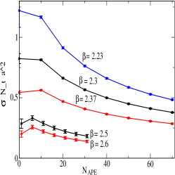
Figure 2: (color online) The effect of smearing on the “string tension” $\sigma$. In confinement ($\beta=2.23,~{}2.3,~{}2.37$) $\sigma$ was obtained from the correlator of Polyakov loops. In deconfinement ($\beta=2.5,~{}2.6$) $\sigma$ was obtained from the behavior of space-like Wilson loops. The lattice size was $20^{3}\times 6$.

For the present investigation at $\beta=2.3$ and the two other $\beta=2.2,~{}2.4$ in the confined phase we adopt this number of smearing steps, justified by the observation that the string tension  at the neighbouring values $\beta=2.23,~{}2.3,~{}2.37$ is reduced after $50$ smearing steps to approximately the same $60\%$ of the original value (see Fig. 2). In the deconfined phase, where the spatial string tension was used for this comparison, the same percentual reduction of this string tension has been observed at $N=25$ and $N=20$ smearing steps for $\beta=2.5,~{}2.6$, respectively.

IV Local Polyakov loop, monopoles and asymptotic holonomy

Our first observation, as in Ref. IMMPV05 , is the correlation between the values of the Polyakov loop and the presence of Abelian monopoles. For this purpose we have averaged the Polyakov loop over all eight corners of a three-dimensional cube (dual to a time-like link of the dual lattice) where an Abelian magnetic charge has been detected. This construction is implied whenever the original and the dual lattice are put into relation. The distribution of the values of this conditionally averaged Polyakov loop is shown in the different panels of Fig. 3 as histograms (with broad 12 bins, drawn in thick lines). For comparison, the distributions of the Polyakov loop over all lattice sites are shown (as fine-binned histograms, drawn in thin lines). One sees that, with $\beta$ approaching the phase transition from the confinement side, the distribution over all lattice sites becomes flatter, whereas the distribution over the position of monopoles becomes increasingly shifted toward $\pm 1$.

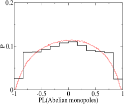
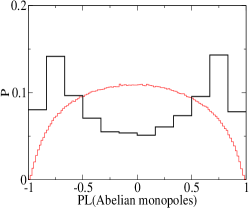
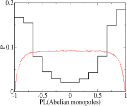
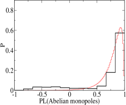
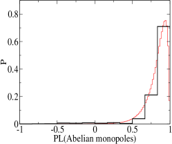
Figure 3: (color online) The distribution of the Polyakov loop over sites where time-like Abelian monopole currents are detected (thick line). Monopoles are obtained by Abelian projection in MAG. For comparison, the distribution of Polyakov loops over all sites is shown (thin line). The upper row of figures shows the results for $\beta=2.2,~{}2.3,~{}2.4$ (from left to right, confinement). The lower row of figures shows the results for $\beta=2.5,~{}2.6$ (from left to right, deconfinement).

Within our set of runs above but not so close to the deconfinement temperature global flips of the Polyakov loop did not happen. Due to this effective $Z(2)$ breaking the two plots for the deconfined phase show an unsymmetric distribution for the Polyakov loop over all lattice sites. At these temperatures the same asymmetry is seen in the distribution of the Polyakov loops for the monopole positions.

In order to facilitate a qualitative comparison of the topological clusters with KvB caloron solutions with nontrivial holonomy $L_{\infty}$, we have defined an empirical asymptotic holonomy $H$ for each lattice configuration. We have considered the sites on the lattice where the absolute value of topological charge density is less than the averaged absolute value of this density. We take the average of the Polyakov loop over this set of asymptotic sites and call the resulting observable the asymptotic holonomy $H$. The distribution of $H$ for the five $\beta$ values is shown in Fig. 4.

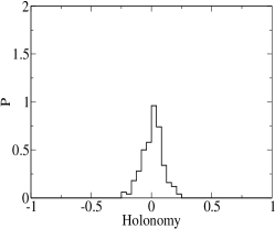
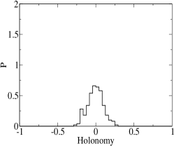
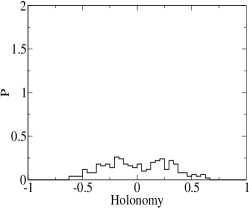
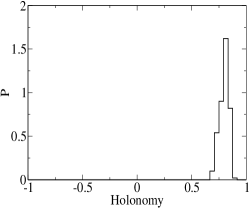
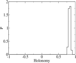
Figure 4: The distribution of the “asymptotic” holonomy $H$ as defined in the text. The upper row of figures shows the results for $\beta=2.2,~{}2.3,~{}2.4$ (from left to right, confinement). The lower row of figures shows the results for $\beta=2.5,~{}2.6$ (from left to right, deconfinement).

It can be seen from the different panels of this figure that the asymptotic holonomy $H$ is concentrated near zero deep in the confined phase ($\beta=2.2$ and 2.3) . The distribution is widened at $\beta=2.4$ , already close to the deconfining transition, and it becomes again concentrated around a maximum moving slowly between $+0.5$ and $+1$ for our temperature range in the deconfined phase.

Note the sharp contrast characteristic for the confinement phase of the $H$ distribution to the Polyakov loop distribution at the positions of time-like monopoles (as defined in MAG) in Fig. 3. In the deconfined phase the local Polyakov loop at the monopole positions is distributed around the asymptotic (global) holonomy $H$.

V Cluster analysis of smeared configurations

On one hand, for each of the four-dimensionally smeared configurations we have looked for clusters of topological charge. The topological density is assigned to the lattice sites according to the unimproved (naive) twisted plaquette definition. In order to form clusters for the subsequent analysis we have selected the sites where the absolute value of the topological charge density exceeds some threshold value $q_{c}$. The link-connected sites with $q(x)>q_{c}$ or $q(x)<-q_{c}$ form what we call positive (negative) clusters of topological charge. Obviously, number and size of the clusters depend on the threshold $q_{c}$. This value has been varied between the ensemble average of $|q(x)|$, taken as lowest threshold, and a value taken $10$ times larger taken as the highest threshold with the aim to get, for each smeared configuration, a maximal number of mutually disconnected clusters of topological charge. Therefore, this procedure finds an upper bound for the number of clusters per configuration (corresponding to the degree of smearing that we have chosen). This number can be inferred from Table I and amounts to 20 to 55 clusters per configuration, maximal at the lowest and highest temperature, minimal at $T\lesssim T_{c}$. Obviously, the number of clusters is not a well-defined quantity, and many of the shallow clusters should be ignored as mere extended background fluctuations.

Table 1: The numbers of topological clusters for $200$ smeared configurations at different $\beta$ identified as static dyons (D), non-static calorons (CAL) and without clear identification (OTHER).

$\beta$	$T/T_{\rm dec}~{}~{}~{}$	$D~{}~{}~{}$	$CAL~{}~{}~{}$	$OTHER~{}~{}~{}$
$2.2~{}~{}~{}$	$0.54~{}~{}~{}$	$39~{}~{}~{}$	$624~{}~{}~{}$	$10323~{}~{}~{}$
$2.3~{}~{}~{}$	$0.68~{}~{}~{}$	$128~{}~{}~{}$	$755~{}~{}~{}$	$6512~{}~{}~{}$
$2.4~{}~{}~{}$	$0.94~{}~{}~{}$	$626~{}~{}~{}$	$511~{}~{}~{}$	$2983~{}~{}~{}$
$2.5~{}~{}~{}$	$1.32~{}~{}~{}$	$243~{}~{}~{}$	$84~{}~{}~{}$	$6989~{}~{}~{}$
$2.6~{}~{}~{}$	$1.87~{}~{}~{}$	$118~{}~{}~{}$	$20~{}~{}~{}$	$10204~{}~{}~{}$

On the other hand, we have identified the complete monopole structure for each smeared configuration. This means that all monopole clusters have been found. A monopole cluster is a connected set of occupied links of the dual lattice, i.e. all links carrying non-vanishing magnetic charge current. The density of monopole currents (i.e. the percentage of occupied links of the dual lattice) in the smeared configurations was about two orders of magnitude smaller than in the corresponding equilibrium ones. Therefore, in the smeared ensemble monopole clusters were mainly non-selfintersecting loops, in the confinement phase yet percolating loops. From the set of all monopole clusters in a configuration, we have selected those isolated monopole loops that are either closed by periodicity in the time direction (then mainly formed by minimal length $L=6$ static time-like monopole currents) or closed within the four-dimensional volume (then mainly with the minimal loop sizes $L=4$, $6$, $8$). If there was a complete covering of exactly one monopole loop (of either kind) with some topological cluster, we have classified this cluster either as a static dyon or as a nondissociated caloron, which are the two opposite appearances of KvB calorons. Table I shows the corresponding numbers of topological clusters classified in one or the other way. Note that our classification, due to the very restrictive cut, has been passed only by a small fraction of topological clusters. The number of topological clusters in general is best defined closely below the phase transition ($\beta=2.4$) where it reaches a minimum of $\approx 15$ per configurations. Approximately one third of them becomes successfully classified as dyons or calorons, the rest has no obvious interpretation in terms of the monopole content. The minimal monopole clusters mentioned above could be intersecting with the large, percolating monopole loops, hence having escaped our attention.

With the 4-dimensional volume of $17.84\mathrm{~{}fm}^{4}$ (at $\beta=2.4$ the lattice spacing is obtained from $\sigma a^{2}=0.071(1)$ LuciniTeper ) the density of identified calorons could be estimated as $0.143\mathrm{~{}fm}^{-4}$, the density of dyons $0.175\mathrm{~{}fm}^{-4}$. The relative abundance extrapolated to the full number of clusters at this $\beta$ would for the calorons result in $0.374\mathrm{~{}fm}^{-4}$, still in the right ballpark given the constant topological susceptibility $\chi\approx 1\mathrm{~{}fm}^{-4}$ below $T_{\rm dec}$. Expressed in physical units, one can summarize the outcome as follows: the density of monopoles (dyons) continuously increases with the temperature. Near the phase transition the densities of calorons and monopole-like objects become comparable. We will discuss below to what extent the monopole-like objects are really dyons and may be described as caloron constituents. The density of objects classified as calorons drops down above the phase transition. This does not come not unexpected in view of the topological susceptibility decreasing with increasing temperature above $T_{\rm dec}$. It remains to be seen whether, in the deconfined phase, the configurations with topological charge $Q=\pm 1$ really contain such a caloron. This would have to be expected from the scenario that calorons are mainly undissociated in the deconfined phase.

Table 2: The densities (in fm^-4) of dyon and caloron clusters, as identified (in the second line extrapolated to the full number of topological charge clusters).

$\beta$	$T/T_{\rm dec}~{}~{}~{}$	$D~{}~{}~{}$	$CAL~{}~{}~{}$
$2.2~{}~{}~{}$	$0.54~{}~{}~{}$	$1.14\cdot 10^{-3}$	$0.0182$
$2.2~{}~{}~{}$	$0.54~{}~{}~{}$	$0.018$	$0.283$
$2.3~{}~{}~{}$	$0.68~{}~{}~{}$	$9.78\cdot 10^{-3}$	$0.0577$
$2.3~{}~{}~{}$	$0.68~{}~{}~{}$	$0.062$	$0.425$
$2.4~{}~{}~{}$	$0.94~{}~{}~{}$	$0.175$	$0.1429$
$2.4~{}~{}~{}$	$0.94~{}~{}~{}$	$0.458$	$0.374$
$2.5~{}~{}~{}$	$1.32~{}~{}~{}$	$0.260$	$0.0900$
$2.5~{}~{}~{}$	$1.32~{}~{}~{}$	$5.55$	$1.92$
$2.6~{}~{}~{}$	$1.87~{}~{}~{}$	$0.514$	$0.0872$
$2.6~{}~{}~{}$	$1.87~{}~{}~{}$	$38$	$6.45$

In order to corroborate (or relativize, for the deconfined phase) this interpretation we have tried to characterize the monopole-tagged clusters by some cluster variables. We have averaged the Polyakov loop inside the selected clusters again over all those sites where time-like Abelian monopole currents of either sign are observed as part of the closed monopole loop that served the identification. We call this quantity the Polyakov loop averaged over the “monopole skeleton” of the given cluster, $\langle PL(\mathrm{Abelian~{}monopoles})\rangle_{cluster}$. From KvB calorons we expect this average for “static monopole clusters” to be close to $~{}\pm 1~{}$, whereas for “monopole–antimonopole pair clusters” it should be close to $~{}0~{}$, the latter because of the internal dipole structure in terms of the Polyakov loop that reflects the positions of the constituents which otherwise would be hidden inside the single undissociated caloron cluster. We use this as the first cluster variable that should quantitatively characterize the type of cluster.

As a second cluster variable we want to consider the topological charge assigned to the cluster. This total charge is difficult to assess because the topological profile extends below the threshold $q_{c}$. Applying this cutoff was, however, indispensable to localize the cluster. We have designed a model-dependent estimator for the total topological charge of an identified topological cluster.

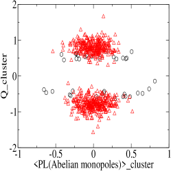
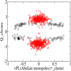
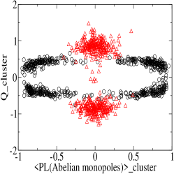
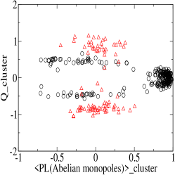
Figure 5: (color online) Scatter plots in the ($Q_{cluster}$,$~{}\langle PL(\mathrm{Abelian~{}monopoles})\rangle_{cluster}$) plane for $\beta=2.2,~{}2.3,~{}2.4$ (upper row from left to right, confinement) and for $\beta=2.5,~{}2.6$ (lower row from left to right, deconfinement). The circles represent dyon clusters, the triangles undissociated calorons.

This estimator works differently for the two types of clusters. For a static dyon we know from the analytic KvB caloron solution that its size depends on the holonomy parameter $\omega$ according to Eq. (1) as

$$\bar{r}=\frac{b}{4\pi\omega}~{}.$$ (2)

$b$ is the inverse temperature, i.e. the period in time direction. In the confinement phase assuming the holonomy parameter to be $\omega=0.25$ the size of the dyons changes inversely to temperature. Actually, the sizes of the dyon clusters are distributed within some width. According to the caloron solution in the limit of separated dyons, the modulus of the topological charge density $q_{max}$ in the center $x_{max}$ of the dyon cluster should be connected with the cluster size in the following way:

$$q_{max}=\frac{1}{24\pi^{2}\bar{r}^{4}}~{}.$$ (3)

Ascribing by this relation a size to each cluster classified as static dyon we could obtain a cluster size distribution from the observed maxima of the topological charge density inside the clusters. Then, considering such a cluster, we sum the actual topological charge over all sites $x$ that belong to the cluster including the tail below $q_{c}$. That means that we sum the topological charge density $q(x)$ within a tube with a 3-dimensional (spatial) radius $R$ (related to $~{}\bar{r}$). This distance $R$ should not be too large in order to avoid double counting of topological charge (by assigning sites to more than one cluster) and not too small (in order not to underestimate the topological charge in the tail of the cluster under consideration). We use $R=3~{}\bar{r}$ which, for the case of an isolated dyonic cluster (with an ideal, approximately exponential topological charge density profile), would estimate the total charge within $7\%$ accuracy. This estimator corrects for the tail and serves to assign a topological charge to all clusters once they have been classified as static dyon clusters.

An undissociated KvB caloron has a topological charge profile like that of an isolated ordinary instanton solution. In this case the maximum of the modulus of the topological charge density is related to the instanton size $~{}\rho~{}$ as follows

$$q_{max}=\frac{6}{\pi^{2}\rho^{4}}~{}.$$ (4)

Assuming that the clusters classified as undissociated calorons have such a charge profile we can obtain the instanton size $~{}\rho~{}$ from the measured $~{}q_{max}~{}$ of the cluster. Then we sum the actual topological charge density over all sites $x$ inside a 4-dimensional ball with a radius $1.5\rho$ centered at $x_{max}$. Finally, the result needs to be multiplied by a correction factor $~{}1.29~{}$ inferred from the exact instanton solution. In this way, we are in the position to define an estimated topological charge for any cluster once it has been identified as undissociated caloron.

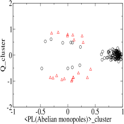
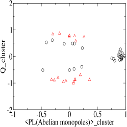
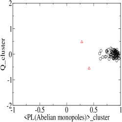
Figure 6: (color online) Scatter plots in the ($Q_{cluster}$,$~{}\langle PL(\mathrm{Abelian~{}monopoles})\rangle_{cluster}$) plane for $\beta=~{}2.6$. The left figure is the sum of the other two. The figure in the center shows configurations (45 from 200 configurations) with topological charge $|Q|=1$ ($0.5\leq|Q|\leq 1.5$), the right figure the complementary 155 configurations with zero topological charge $Q=0$ ($|Q|\leq 0.5$). The meaning of the symbols is the same as in Fig. 5.

We show in Fig. 5 scatter plots showing clusters of our topological clusters in the plane spanned by the estimated topological charge of each cluster, $~{}Q_{cluster}~{}$, and the Polyakov loop averaged over the monopole skeleton, denoted as $\langle PL(\mathrm{Abelian~{}monopoles})\rangle_{cluster}$. The points in these scatter plots represent cluster that have been identified in one or the other way. As it can be seen from this figure, in the confined phase with increasing $\beta$ (here at $\beta=2.3,~{}2.4$) the two sorts of topological clusters are forming clusters on the scatter plot either closer to the points $~{}\langle PL(\mathrm{Abelian~{}monopoles})\rangle_{cluster}=\pm c,~{}Q_{cluster}=\pm 1/2~{}$ (dissociated) or $~{}\langle PL(\mathrm{Abelian~{}monopoles})\rangle_{cluster}=0,~{}Q_{cluster}=\pm 1~{}$ (undissociated), with $c\to 1$ with increasing temperature. In the confined phase at lower temperature, $\beta=2.2$, clusters which contain closed monopole loops (“undissociated calorons”) are the most abundant objects (among the identified ones) and are forming a cluster, very similarly to $\beta=2.3,~{}2.4$ . On the other hand, dissociated dyons are very rare and have not yet produced a pronounced pattern of non-vanishing Polyakov loop (when the Polyakov loop is averaged over the monopole skeleton of the cluster).

In the deconfined phase at $\beta=2.5,~{}2.6$ undissociated calorons are forming clusters in the same way as they do in the confined phase. However, they become increasingly rare objects with increasing temperature. Single (dissociated) dyons are presented now by asymmetric objects: rare heavy dyons with an averaged Polyakov line of opposite sign compared to the holonomy $H$ and frequent light dyons with averaged Polyakov line approximately equal to the value of the asymptotic holonomy. Undissociated calorons and heavy dyons are appearing almost exclusively in configurations with total topological charge equal to $Q=\pm 1$ while light dyons appear mainly in configurations with total topological charge equal to $Q=0$ and to a lesser extent in $Q=\pm 1$ configurations (see Fig. 6). The charge values $Q=0,\pm 1$ exhaust all cases among the smeared configurations on the given lattice size, that are found for the two $\beta$-values in the deconfined phase. This suggests to view the topological background in the deconfined phase mainly as a gas of “spurious” (both with small action and topological charge) dyon–antidyon pairs. These pairs cannot be understood as forming together a caloron. If they were related to calorons at all, more likely they have emerged from a caloron-anticaloron pair by annihilation of their heavy partners. For these dyons it has to be checked whether they are formed by locally selfdual or anti-selfdual field. Modeling the size of these objects starting from the topological density in the center is more questionable than in the other cases. Considered only as static Abelian magnetic monopoles, they do not have to follow the dyonic interpretation. However they could be held responsible for the magnetic confinement. From this point of view it is no surprise that their density increases with temperature above $T_{\rm dec}$.

Under further cooling, pairs of dyons and antidyons in this gas can eventually annihilate. In some cases (when the annihilation proceeds across the periodic boundary) this process ends up with Dirac sheets (i.e. constant magnetic fluxes) Dirac_sheets_we . These Dirac sheets are either stable or unstable depending on the value of holonomy Stability_PvB .

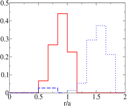
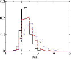
Figure 7: (color online) Left: distributions of the radii $\bar{r}$ of dyonic clusters for $\beta=2.3$ (solid lines, confinement phase) and $\beta=2.6$ (dashed/dotted lines, deconfinement phase). The dashed line corresponds to heavy dyon clusters, whereas the dotted line refers to light dyons. Right: distributions of the scale-sizes $\rho$ of isolated caloron clusters for $\beta=2.2$ (solid line), $\beta=2.3$ (dashed line), and $\beta=2.4$ (dotted line). Both the values for $\bar{r}$ and $\rho$ are presented in units of the lattice spacing $a(\beta)$.

With some reservations concerning the dyonic interpretation of the monopole-like clusters in the deconfined phase, we have made a comparison of the “dyon” radii found in the confined and deconfined phases. In the left half of Fig. 7 we show the size distributions derived from the $q_{max}$-values of clusters classified as single dyons. For the confinement phase, this yields a distribution with a single maximum as expected from the caloron model taken seriously. In the deconfined phase, the discrimination between the abundant light dyon clusters with the same sign of the Polyakov loop at the monopole position and the rare heavy dyon clusters with opposite sign, always with respect to $H$, is reflected in the figure and highlighted by dotted and dashed lines, respectively. For comparison, we show in the right part of Fig. 7 the $\rho$ distributions of isolated single caloron clusters found in the confinement phase. These distributions undoubtedly reflect the increasing size of the objects yet to be classified as single calorons. This tendency fits together with the increasing amount of dyons since, with increasing size, calorons eventually turn into discernible dyons.

According to the relation (2), an estimate of $\omega=0.25$ for maximally nontrivial holonomy at $\beta=~{}2.3$, and $\omega=0.1$ corresponding to $\langle H\rangle=0.8$ at $\beta=~{}2.6$ could be taken for rough orientation. Since the inverse temperature is $b=6a$ (with $N_{\tau}=6$) in all our cases, we would estimate $\bar{r}\approx 2\times a(\beta)$ for all dyonic constituents in the confined phase, whereas at $\beta=~{}2.6$ in the deconfined phase the light dyons should have a typical radius $\bar{r}=~{}4.8\times a(2.6)$ and the heavy dyons (with $\omega$ replaced by $\bar{\omega}=0.5-\omega=0.4$) a radius of $\bar{r}=~{}1.2\times a(2.6)$. Notice that the lattice spacings for the two $\beta$-values are widely different (they differ by a factor 2.75). Taking this into account the dyons at $\beta=~{}2.3$ (equally weighted in the confinement phase) would have a size of $\bar{r}\approx~{}0.6/\sqrt{\sigma}$, that happens to be almost equal to the size of the light dyons at $\beta=~{}2.6$ (in the deconfined phase) which is $\bar{r}\approx~{}0.64/\sqrt{\sigma}$. The heavier dyons at $\beta=~{}2.6$ in the deconfined phase (which are actually rather rare) would be 4-times smaller in size, namely $\bar{r}\approx 0.16/\sqrt{\sigma}$. For the lattice spacings $a(\beta)$ assumed here in order to express all sizes in terms of the $SU(2)$ string tension at $T=0$ we refer to Ref. LuciniTeper .

Concluding we can say that the distributions drawn in Fig. 7 do not agree quantitatively with the above estimates dictated by holonomy values $H\equiv L_{\infty}$, but show at least qualitatively the expected pattern of size splitting. On one hand, the averaged holonomy $H$ might not be a relevant parameter for the asymptotics of a single topological cluster. On the other hand, we would not take these caloron-based estimates too serious for the static monopoles seen in the deconfined phase, because they are not observed in heavy-light pairs and are badly modelled by the formula for calorons and selfdual BPS dyons.

VI Conclusion

We have analyzed the topological clusters of four-dimensionally smeared configurations at finite temperatures, across the deconfining phase transition, by means of studying the monopole-worldline cluster content of these clusters. This tool has allowed to identify part of the topological clusters either as static dyons or non-static calorons. We have to stress, however, that the number of separable topological clusters was maximized in the course of analysis such that a huge part of the clusters (more than 90 % at the lowest temperature and in the deconfined phase, approximately 70 % closely below the transition temperature) remained unidentified in this sense. This doesn’t mean that they couldn’t be classified using other means. The simple monopole clusters that were thought to identify clusters as dyons or calorons could have been intersecting with the percolating part that exists in the confinement phase. Another part of the topological clusters, mainly in the deconfined phase, should simply have been ignored because they are shallow background fluctuations. These have nothing to do whatsoever with the well-localized, (anti)selfdual carriers of topological charge which had to be analyzed.

On the basis of this separation we attempted a model-dependent reconstruction of the total topological charge for each individual cluster. The correlation between the Polyakov loop (averaged over the monopole skeleton) and the total topological cluster charge has revealed the following pattern. At temperatures not too much below the deconfining phase transition, with the asymptotic holonomy being still maximally nontrivial, $H=0$, we see both nondissociated calorons and separate dyons, understood as the result of part of the calorons being already dissociated into dyons. The size of the nondissociated ones slightly increases with temperature. Dyons with different local values of the Polyakov loop are symmetric in mass and action in the confinement phase. The ratio of the number of dyons to the number of (yet undissociated) calorons is increasing with temperature, such that we may speak about a process of dissociation with increasing temperature. At the transition temperature the densities of both objects has become comparable.

Above the deconfining phase transition holonomy starts to become trivial, $H\neq 0$. Contrary to our expectations topological excitations are not dominated by (undissociated or dissociated) calorons. Only half of the $Q=\pm 1$ configurations can be interpreted as undissociated calorons. Judged solely from the average Polyakov loop at the static clusters, dyons are still prevailing above $T_{dec}$. The most abundant objects are light dyons and antidyons with static Abelian monopoles inside. That dyons are no more symmetric in mass and action would have been expected. But they do not appear anymore as pairs of light and heavy constituents in the same configuration. Therefore it is difficult to understand these configurations as dissociated calorons.

The typical $Q=0$ configurations contains monopole–antimonopole pairs, each with only insignificant topological charge. Since the estimate of the charge rests on formulae for BPS dyons, some reservations about the topological charge are due. Considered simply as static magnetic monopoles (ignoring the topological charge cluster) together with other magnetic monopoles they could be held responsible for the spatial string tension (magnetic confinement) in the deconfined phase. From this point of view it is plausible that the density of monopoles does not follow the decline of the topological susceptibility above $T_{\rm dec}$.

The logical next step will be to repeat the present study with a suitable fermionic topological charge density applied to the (unsmeared) equilibrium gauge field configurations with the option of eliminating UV fluctuations by mode truncation.

References

- (1)
- (2)
- (3) E.-M. Ilgenfritz, B. V. Martemyanov, M. Müller-Preussker, and A. I. Veselov, Phys. Rev. D71, 034505 (2005).
- (4) T. DeGrand, A. Hasenfratz, and T. G. Kovacs, Nucl. Phys. B520, 301 (1998).
- (5) T. C. Kraan and P. van Baal, Phys. Lett. B435, 389 (1998).
- (6) T. C. Kraan and P. van Baal, Nucl. Phys. B533, 627 (1998).
- (7) K. Lee and C. Lu, Phys. Rev. D58, 025011 (1998).
-
(8)
M. K. Prasad and C. M. Sommerfield, Phys. Rev. Lett. 35, 760 (1975);
E. B. Bogomol’nyi, Sov. J. Nucl. Phys. 24, 449 (1976). - (9) R. C. Brower, D. Chen, J. Negele, K. Orginos, and C-I Tan, Nucl. Phys. Proc. Suppl. 73, 557 (1999).
- (10) E.-M. Ilgenfritz, B. V. Martemyanov, M. Müller-Preussker, and A. I. Veselov, Phys. Rev. D69, 114505 (2004).
- (11) C. Gattringer, E.-M. Ilgenfritz, and S. Solbrig, e-Print Archive: hep-lat/0601015.
- (12) G. S. Bali, V. G. Bornyakov, M. Müller-Preussker, and K. Schilling, Phys. Rev. D54, 2863 (1996).
- (13) D. Diakonov, N. Gromov, V. Petrov and S. Slizovskiy, Phys. Rev. D70, 036003 (2004).
- (14) D. Diakonov, Prog. Part. Nucl. Phys. 51, 173 (2003).
- (15) M. García Pérez, A. González-Arroyo, C. Pena, and P. van Baal, Phys. Rev. D60, 031901 (1999).
- (16) M. N. Chernodub, T. C. Kraan, and P. van Baal, Nucl. Phys. Proc. Suppl. 83, 556 (2000).
- (17) E.-M. Ilgenfritz, B. V. Martemyanov, M. Müller-Preussker, S. Shcheredin, and A. I. Veselov, Phys. Rev. D66, 074503 (2002).
- (18) E.-M. Ilgenfritz, M. Müller-Preussker, and D. Peschka, Phys. Rev. D71, 116003 (2005).
- (19) C. Gattringer and S. Schaefer, Nucl. Phys. B654, 30 (2003).
- (20) C. Gattringer and R. Pullirsch, Phys. Rev. D69, 094510 (2004).
- (21) C. Gattringer and S. Solbrig, Talk presented at 11th International Conference in Quantum ChromoDynamics (QCD 04), Montpellier, France, 5-9 Jul 2004, e-Print Archive: hep-lat/0410040.
- (22) C. Gattringer, E.-M. Ilgenfritz, B. V. Martemyanov, M. Müller-Preussker, D. Peschka, R. Pullirsch, S. Schaefer, and A. Schäfer, Nucl. Phys. Proc. Suppl. 129, 653 (2004).
- (23) P. Hasenfratz, V. Laliena, and F. Niedermayer, Phys. Lett. B427, 125 (1998).
- (24) Y. Koma, E.-M. Ilgenfritz, K. Koller, G. Schierholz, T. Streuer, and V. Weinberg, Proc. of Science LAT2005 300, 2005 (.)
- (25) V. Weinberg, E.-M. Ilgenfritz, K. Koller, Y. Koma, G. Schierholz, and T. Streuer, Proc. of Science LAT2005 171, 2005 (.)
- (26) E.-M. Ilgenfritz, K. Koller, Y. Koma, G. Schierholz, T. Streuer, and V. Weinberg, Nucl. Phys. Proc. Suppl. 153, 328 (2006).
- (27) F. Bruckmann, E.-M. Ilgenfritz, B. V. Martemyanov, and P. van Baal, Phys. Rev. D70, 105013 (2004).
- (28) E.-M. Ilgenfritz, B. V. Martemyanov, M. Müller-Preussker, and A. I. Veselov, EPC34, 439 (2004).
- (29) E.-M. Ilgenfritz, M. Müller-Preussker, B. V. Martemyanov, and P. van Baal, Phys. Rev. D69, 097901 (2004).
- (30) B. Lucini and M. Teper, JHEP 0106, 050 (2001).