On the Continuum Limit of Topological Charge Density Distribution

Abstract

The bulk distribution of the topological charge density, constructed via ${\mathrm{HP}^{1}}$ $\sigma$-model embedding method, is investigated. We argue that the specific pattern of leading power corrections to gluon condensate hints on a particular UV divergent structure of ${\mathrm{HP}^{1}}$ $\sigma$-model fields, which in turn implies the linear divergence of the corresponding topological density in the continuum limit. We show that under testable assumptions the topological charge is to be distributed within three-dimensional sign-coherent domains and conversely, the dimensionality of sign-coherent regions dictates the leading divergence of the topological density. Confronting the proposed scenario with lattice data we present evidence for indeed peculiar divergence of the embedded fields. Then the UV behavior of the topological density is studied directly and is found to agree with our proposition. Finally, we introduce parameter-free method to investigate the dimensionality of relevant topological fluctuations and show that indeed topological charge sign-coherent regions are likely to be three-dimensional.

I Introduction

Topology investigations had always been conspicuous topic for the lattice community and the recent advances indeed put it on the solid grounds. Both the topological charge and its density are now computable on thermalized vacuum configurations and the results already obtained in pure Yang-Mills theories indicate that the conventional instanton based models are to be strongly modified. Here we basically mean the discovery of global topological charge sign-coherent regions Horvath:2005rv and, what is even more important for us, the lower dimensionality of these regions Horvath:2005rv ; Aubin:2004mp ; Ilgenfritz:2005hh ; Horvath:2005cv ; Gubarev:2005jm ; Zakharov:2006vt , which are now believed to be three-dimensional. Note that the lower dimensionality of physically relevant vacuum fluctuations should not come completely unexpected, it had been repeatedly discussed in the recent past (see, e.g., Refs. Kovalenko:2005zx ; Bornyakov:2001hs ; Gubarev:2002ek ).

It is important that qualitatively the same picture of relevant topological fluctuations appeared recently within radically different approach introduced and developed in Refs. Gubarev:2005rs ; Boyko:2005rb . Without mentioning all the details and technicalities involved we note only that the ${\mathrm{HP}^{1}}$ embedding method is the nearest to the classical ADHM investigation of $SU(2)$ gauge fields topology and essentially reconstructs the topology defining map $S^{4}\to{\mathrm{HP}^{1}}=S^{4}$, in terms of which both the topological charge and its density obtain unambiguous and well defined meaning. We are not in the position to review all the results obtained in Gubarev:2005rs ; Boyko:2005rb , however, it is important that ${\mathrm{HP}^{1}}$ embedding allows to get rid of leading perturbative divergences in various observables. Moreover, it reproduces the topological aspects of $SU(2)$ Yang-Mills theory, is fairly compatible with other topology investigation approaches and allows to calculate with amazing accuracy the gluon condensate, demonstrating firmly that its quadratic power correction does not vanish. It is crucial that the only non-trivial power dependence of ${\mathrm{HP}^{1}}$ projected curvature upon UV cutoff is contained in the quadratic term, which must be encoded in the local structure of the topology defining map $S^{4}\to{\mathrm{HP}^{1}}$. In section II.1 we argue that the only possibility to reproduce the observed pattern of power corrections is to assume that the mapping $S^{4}\to{\mathrm{HP}^{1}}$ is highly asymmetric so that the corresponding Jacobian (which is essentially equivalent to the topological density) diverges linearly with diminishing lattice spacing. In turn this divergence implies rather peculiar geometry of the relevant topological excitations. Namely, we show in section II.2 that the topological charge sign-coherent regions are to be three-dimensional domains embedded into original four-dimensional space. Here the consistency check is provided by the fluctuations of topological charges associated with sign-coherent regions.

Attempt to confront the above scenario with the lattice data brings out a wealth of both technical and theoretical issues, which are addressed in section III. In section III.1 we present numerical measurements which justify our conclusion about the local structure of the map $S^{4}\to{\mathrm{HP}^{1}}$. The direct measurement of the UV behavior of the topological density (sections III.2, III.3) necessitates the invention of new calculation algorithm, which turns out to be fast and rather accurate. It allows us to make statistically significant comparison of the theoretical considerations with lattice data and confirms that the characteristic topological density is indeed divergent, but at most linearly, in the continuum limit. As far as the dimensionality of relevant fluctuations is concerned, we investigate it in section III.4 and develop unambiguous, in fact, method of its determination. Essentially it is the specially crafted biased random walk model embedded into the ambient topological density environment. We argue that the appearance of critical-like behavior of the model signifies the lower dimensional long-range order present in the topological density background. We show that critical regime does occur and indicates that indeed the density is concentrated in highly extended submanifolds, the dimensionality of which is compatible with three. Finally we investigate the fluctuations of the topological charges associated with sign-coherent regions and argue that only three-dimensional domains with linearly divergent topological density are consistent with theoretical and experimental restrictions imposed on the structure of topological fluctuations.

II Scaling of Topological Density

II.1 Gluon Condensate, Leading Power Correction and Divergence of Topological Density

The essence of ${\mathrm{HP}^{1}}$ $\sigma$-model embedding approach is the assignment of unique configuration of ${\mathrm{HP}^{1}}$ $\sigma$-model fields $|\,q_{x}\,\rangle$ to every given SU(2) gauge background $A_{\mu}$ (until section III we use continuum notations), where $|\,q_{x}\,\rangle$ is two-component, normalized $\langle\,q_{x}\,|\,q_{x}\,\rangle=1$, quaternionic vector (see Refs. Gubarev:2005rs ; Boyko:2005rb for details). The relevant configuration $|\,q_{x}\,\rangle$ is defined by the requirement that it provides the absolute minimum to the functional

$$F(A,q)~{}=~{}\int d^{4}x\,\mathop{\rm Tr}\left(A_{\mu}~{}+~{}\langle\,q\,|\partial_{\mu}|\,q\,\rangle\right)^{2}$$ (1)

for given (fixed) gauge potentials $A_{\mu}$. Note that gauge covariance is maintained exactly since the $\sigma$-model target space ${\mathrm{HP}^{1}}$ is the set of equivalence classes with respect to $|\,q_{x}\,\rangle\sim|\,q_{x}\,\rangle\,\upsilon_{x}$, $\upsilon_{x}\in SU(2)$. The uniqueness of the minimum of (1) and the factual absence of Gribov copies problem was discussed in length in Refs. Gubarev:2005rs ; Boyko:2005rb and here we take it for granted. Therefore the embedded ${\mathrm{HP}^{1}}$ $\sigma$-model fields $|\,q_{x}\,\rangle$ are unique (although non-local) functions of the original potentials. The advantage of the construction is that the gauge fields topology becomes explicit in terms of $|\,q_{x}\,\rangle$ variables. Indeed, the gauge invariant projectors $|\,q_{x}\,\rangle\langle\,q_{x}\,|$ provide the map of compactified physical space $S^{4}$ into the target space ${\mathrm{HP}^{1}}$, the degree of which is equal to the topological charge of the original gauge background. Furthermore, the local distinction of this map from trivial one is the uniquely defined measure of the topological charge density. One could say that the sole purpose of ${\mathrm{HP}^{1}}$ embedding method is to locally reconstruct the topology defining map $S^{4}\to{\mathrm{HP}^{1}}$, which allows to get essentially all the topological aspects of the original background.

Then it is natural to introduce the ${\mathrm{HP}^{1}}$ projection

$$A_{\mu}~{}\to~{}A^{\mathrm{HP}}_{\mu}~{}\equiv~{}-\langle\,q\,|\partial_{\mu}|\,q\,\rangle\,,$$ (2)

which replaces $A_{\mu}$ with its best possible approximation by $\sigma$-model induced potentials. The striking properties of the projected fields $A^{\mathrm{HP}}_{\mu}$ were investigated in details in Ref. Boyko:2005rb . In particular, it was shown that $A^{\mathrm{HP}}_{\mu}$ exactly reproduce the most of non-perturbative aspects of the original $SU(2)$ configurations, while containing no sign whatsoever of usual perturbative divergences. To the contrary, the kernel of the map (2) was shown to correspond to pure perturbation theory with identically trivial topology and vanishing string tension. Without mentioning all the aspects and properties of ${\mathrm{HP}^{1}}$ projection (2) let us note that it allows to calculate with inaccessible so far accuracy the gluon condensate and its leading power correction. Indeed, the spacing dependence of ${\mathrm{HP}^{1}}$ projected gauge curvature $F^{\mathrm{HP}}_{\mu\nu}$ was found to be astonishingly well described by

$$\langle\;{1\over 2}\mathop{\rm Tr}(F^{\mathrm{HP}}_{\mu\nu})^{2}\rangle~{}=~{}\frac{4\alpha_{2}}{a^{2}}~{}+~{}\frac{\pi^{2}}{6}\,\langle\frac{\alpha_{s}}{\pi}G^{2}\rangle\,,$$ (3)

$$\alpha_{2} = [61(3)\mathrm{~{}MeV}]^{2}\,,$$ (4)

$$\langle\frac{\alpha_{s}}{\pi}G^{2}\rangle\ = 0.0271(10)\mathrm{~{}GeV}^{4}\,,$$

where $a$ is the lattice spacing ($1/a$ servers as the UV cutoff). It is crucial that Eq. (3) does not contain any sign of usual perturbative contribution of order $O(a^{-4})$. Note that the value of $\alpha_{2}$ coefficient turns out to be unexpectedly small, nevertheless it fits nicely into the known bounds on the magnitude of the quadratic correction term (see Ref. Rakow:2005yn for recent review). While the actual numbers quoted in (4) are not important for the present discussion, it is crucial that they both are definitely non-zero and therefore the spacing dependence of $\langle\mathop{\rm Tr}(F^{\mathrm{HP}}_{\mu\nu})^{2}\rangle$ includes only $O(a^{-2})$ and $O(a^{0})$ terms.

To analyze the consequences of Eq. (3) let us consider point $n\in S^{4}$, in the neighborhood of which the map $S^{4}\to{\mathrm{HP}^{1}}$ is non-degenerate. In the vicinity of $n$ and its image $m\in{\mathrm{HP}^{1}}$ we introduce local coordinates $x^{\mu}$ and $y^{\mu}$, $\mu=0,...,3$ (stereographic projection from points $n$ and $m$ correspondingly) such that $y_{\mu}(x=0)=0$. Non-degeneracy means that $\mathrm{det}[\partial y/\partial x]\neq 0$ and hence the function $y(x)$ is invertible. From the specific explicit form of ${\mathrm{HP}^{1}}$ projected fields (2) we conclude that

$$A^{\mathrm{HP}}_{\mu}(x)=-\langle\,q_{x}\,|\frac{\partial}{\partial x^{\mu}}|\,q_{x}\,\rangle=J^{\nu}_{\mu}(x)\,A^{inst}_{\nu}(y(x))\,,$$ (5)

where $J^{\mu}_{\nu}=\partial y^{\mu}/\partial x^{\nu}$ is the Jacobian matrix, $A^{inst}_{\mu}(y)$ is the potential of classical BPST instanton solution with unit radius

$$A^{inst}_{\mu}(y)=-\langle\,q\,|\partial_{\mu}|\,q\,\rangle=\frac{(\bar{e}_{\mu}e_{\nu}-\bar{e}_{\nu}e_{\mu})\,y^{\nu}}{2\,(1+y^{2})}$$ (6)

and $e_{\mu}$ denotes quaternionic basis. Note that Eq. (5) is local and crucially depends upon the space-time varying matrix $J^{\nu}_{\mu}$. Furthermore, Eq. (5) relies heavily on the ${\mathrm{HP}^{1}}$ projection (2) and would not be valid for generic gauge potentials. The corresponding ${\mathrm{HP}^{1}}$ projected curvature is similarly expressible in terms of instantonic field-strength

$$F^{\mathrm{HP}}_{\mu\nu}~{}=~{}J^{\rho_{1}}_{\mu}\,J^{\rho_{2}}_{\nu}\,F^{inst}_{\rho_{1}\rho_{2}}\,,$$ (7)

and therefore at point $n\in S^{4}$ we have

$$\;{1\over 2}\mathop{\rm Tr}(F^{\mathrm{HP}}_{\mu\nu})^{2}~{}\propto~{}(\mathop{\rm Tr}g)^{2}~{}-~{}\mathop{\rm Tr}g^{2}\,,$$ (8)

where we have introduced the metric $g^{\mu\nu}=J^{\mu}_{\lambda}J^{\nu}_{\lambda}$ and skipped inessential numerical factor. Therefore the study of the projected curvature ${\langle\;{1\over 2}\mathop{\rm Tr}(F^{\mathrm{HP}}_{\mu\nu})^{2}\rangle}$ is equivalent to the local investigation of the metric $g$ associated with the topology defining map $S^{4}\to{\mathrm{HP}^{1}}$. In term of strictly positive eigenvalues $\lambda_{\mu}$ of $g$, Eqs. (3) and (8) imply

$$\sum\limits_{\mu<\nu}{\langle\lambda_{\mu}\lambda_{\nu}\rangle}~{}=~{}A~{}+~{}B\cdot a^{-2}\,,$$

$$A\sim\Lambda^{4}_{QCD}\,,\quad B\sim\Lambda^{2}_{QCD}\,,$$

where we have generically indicated the IR physical scale involved in Eq. (3) by $\Lambda_{QCD}$ and explicitly kept all powers of lattice spacing. Evidently, Eq. (II.1) imposes rather stringent restrictions on the distribution of eigenvalues $\lambda_{\mu}$ and requires them to depend highly non-trivially upon the UV cutoff. However, Eq. (II.1) is not sufficient to analyze this dependence in details. The relation, which provides an additional input and which is verified numerically in section III.1, reads

$$\sum\limits_{\mu}{\langle\lambda_{\mu}\rangle}~{}=~{}\alpha~{}+~{}\beta\cdot a^{-2}\,,$$ (10)

$$\alpha\sim\Lambda^{2}_{QCD}\,,\quad\beta\sim 1\,.$$

Taken at face value it indicates that generically all the eigenvalues are quadratically divergent in the limit $a\to 0$. However, it turns out that the simplest ansatz

$${\langle\lambda_{0}\rangle}=\beta\cdot a^{-2}\,,\quad{\langle\lambda_{i}\rangle}=\alpha_{i}\,,\quad i=1,2,3\,,$$ (11)

$$\alpha_{i}\sim\Lambda^{2}_{QCD}\,,\quad\sum_{i}\alpha_{i}=\alpha\,,$$

is capable not only to reproduce the observed pattern of power corrections (II.1), (10), but also passes stringent consistency check, which we describe next. Note that without loss of generality the divergent behavior was ascribed to the first eigenvalue. However, it is clear that any particular enumeration of $\lambda_{\mu}$ has no invariant meaning. What is actually meant in Eq. (11) is that only one eigenvalue is quadratically divergent, but it is not possible to assign a particular number to it before averaging. In order to convince the reader that (11) is compatible with both (II.1) and (10) we note that since $\lambda_{0}$ and $\lambda_{i}$ depend upon completely different scales it is legitimate to write $\sum{\langle\lambda_{\mu}\lambda_{\nu}\rangle}={\langle\lambda_{0}\rangle}\sum{\langle\lambda_{i}\rangle}+\sum{\langle\lambda_{i}\lambda_{j}\rangle}$. Then Eq. (II.1) becomes

$$\alpha\,\beta\cdot a^{-2}+\sum\limits_{i<j}{\langle\lambda_{i}\lambda_{j}\rangle}=A+B\cdot a^{-2}$$ (12)

and under quite natural (in view of (11)) assumption $\sum{\langle\lambda_{i}\lambda_{j}\rangle}\sim\Lambda^{4}_{QCD}$ it leads to indeed stringent relation between various coefficients

$$\alpha\cdot\beta~{}=~{}B\,.$$ (13)

It is evident that this equality is highly non-trivial and is not guaranteed a priori. If confirmed by lattice measurements it would imply the validity of the ansatz (11) thus providing the mean to check its self-consistency. As is discussed in section III.1, Eq. (13) is strongly supported by the measurements and is fulfilled with rather amazing accuracy. Moreover, in that section we also consider along the same lines the triple correlator $\sum_{\mu<\nu<\rho}{\langle\lambda_{\mu}\lambda_{\nu}\lambda_{\rho}\rangle}$, for which the analogous to (II.1) relation holds and which provides the additional consistency check similar to (13). Note, however, that in the latter case the numerical uncertainties are larger and for this reason we do not consider the triple correlator here.

To summarize, we found that the ansatz (11) reproduces precisely the observed pattern of leading power divergences (3), (II.1), (10) and is fairly compatible with measured local characteristics of the topology defining map $S^{4}\to{\mathrm{HP}^{1}}$. Since even the relation (13) is strongly supported by the data, we are confident that Eq. (11) reflects correctly the leading UV dependence of the map $S^{4}\to{\mathrm{HP}^{1}}$, which therefore turns out to be highly asymmetric on average. It is worth to note that the standard picture implies $\langle\lambda_{\mu}\rangle\propto\Lambda^{2}_{QCD}$ meaning that unit topological charge is gathered at large (of order $\Lambda^{-1}_{QCD}$) distances. The singular behavior of one eigenvalue $\langle\lambda_{0}\rangle\propto 1/a^{2}$ signifies immediately that the topological susceptibility $\chi={\langle Q^{2}\rangle}/V$ is saturated on submanifolds with characteristic four-volume of order $a\cdot\Lambda^{-3}_{QCD}$. In other words the topological density is to be concentrated mostly in three-dimensional domains embedded into Euclidean four-dimensional space (we return to this problem in section II.2).

The above results have rather dramatic consequences for the topological density $q_{x}$, to illustrate which let us consider ${\langle q^{2}\rangle}$ defined as ${\langle q^{2}\rangle}=\lim_{|x|\to 0}\langle q_{0}q_{x}\rangle$. Note that within the usual approaches this definition is, in fact, ambiguous since the correlation function ${\langle q_{0}q_{x}\rangle}$ is perturbatively dominated at small distances $\langle q_{0}q_{x}\rangle\sim-1/|x|^{8}$. Hence the perturbative ambiguities make the value of $\langle q^{2}\rangle$ undefined and the standard lore is to fix it by the requirement $\chi=\int\langle q_{0}q_{x}\rangle$. However, it is crucial that the ${\mathrm{HP}^{1}}$ embedding approach to the gauge fields topology is factually exempt from perturbation theory. The best illustration is provided by Eq. (3) and in connection with topological density correlation function we discuss this in section III.3. Therefore for ${\mathrm{HP}^{1}}$-based topological density, which in the continuum limit is given by $q\propto\mathop{\rm Tr}F^{\mathrm{HP}}\tilde{F}^{\mathrm{HP}}$, the estimate ${\langle q_{0}q_{x}\rangle}\sim-1/|x|^{8}$ is not valid and UV behavior of ${\langle q^{2}\rangle}$ should be considered anew. Note also that the possible UV divergence of ${\langle q^{2}\rangle}$ could not be subtracted as usual and is not equivalent to conventional contact terms. From now on and throughout the paper the topological density $q_{x}$ is always understood via ${\mathrm{HP}^{1}}$ embedding approach.

In fact, the leading UV behavior of ${\mathrm{HP}^{1}}$-based topological density could be established from Eq. (7). Indeed, from the well known properties of instanton solution it follows that

$$q\propto\mathop{\rm Tr}F^{\mathrm{HP}}\tilde{F}^{\mathrm{HP}}\propto\mathrm{det}\,J=\pm\mathrm{det}^{1/2}\,g\,.$$ (14)

Here it is convenient to introduce the notion of characteristic topological density $\bar{q}$, which could be defined rigorously as $\bar{q}^{2}={\langle q^{2}\rangle}$. However, below we’ll sometimes use this term and the same symbol $\bar{q}$ to denote just the typical scale of the topological density fluctuations. The justification is that as far as the dependence on UV and IR scales is concerned these definitions essentially coincide. Therefore, from Eq. (14) we conclude that

$$\bar{q}^{2}\equiv\langle q^{2}\rangle\propto\langle\mathrm{det}\,g\rangle=\langle\prod\limits_{\mu}\lambda_{\mu}\rangle\sim\frac{\Lambda^{6}_{QCD}}{a^{2}}\,,$$ (15)

where Eq. (11) had been used. The conclusion is that even the non-perturbatively defined topological density is divergent in the continuum limit reflecting directly the highly asymmetric local structure of the topology defining map $S^{4}\to{\mathrm{HP}^{1}}$. Note however that this divergence is incomparable with usual perturbative one $\langle q^{2}\rangle\sim 1/a^{8}$, which, in fact, is even non-integrable. Of course, it is understood that the very definition of the topological density is arbitrary to large extent (full derivative could always be added). However, the ${\mathrm{HP}^{1}}$ embedding method is specified completely with no free parameters involved. Moreover, the corresponding topological density is definitely exempt from perturbative ambiguities so that the divergence (15) could not be equivalent to the contact term and should be dealt with accurately. In particular, we argue in the next section that Eq. (15) implies rather peculiar geometry of vacuum topological fluctuations.

II.2 Dimensionality of Topological Fluctuations

The problem to be addressed in this section is the geometrical properties of vacuum topological fluctuations and in particular their dimensionality. First, let us note that any particular distribution of topological density in finite volume $V$ could be divided unambiguously into the regions $V_{+}$ ($q_{x}>0$) and $V_{-}$ ($q_{x}<0$) of sign-coherent topological charge so that the total charge is given by

$$Q=\int q=\int_{V_{+}}\!\!q~{}+\int_{V_{-}}\!\!q\equiv Q_{+}-Q_{-}\,,$$ (16)

where the relative sign of $Q_{+}$, $Q_{-}$ was made explicit in the last equality ($Q_{-}>0$) and no specific properties of the regions $V_{+}$, $V_{-}$ were supposed ($V_{\pm}$ could be disconnected, in particular). Note that in this section we do assume that the charges $Q_{\pm}$ could be estimated as $Q_{\pm}=\bar{q}\,V_{\pm}$. For mean squared topological charge the decomposition (16) implies

$${\langle Q^{2}\rangle}~{}\propto~{}{\langle Q^{2}_{+}\rangle}-{\langle Q_{+}Q_{-}\rangle}\,,$$ (17)

where we have generically assumed that ${\langle Q^{2}_{-}\rangle}={\langle Q^{2}_{+}\rangle}$. Since the topological susceptibility $\chi$ is a priori postulated to be finite in the continuum limit, we have

$$\frac{{\langle Q^{2}_{+}\rangle}-{\langle Q_{+}Q_{-}\rangle}}{V}=\bar{q}^{2}\frac{{\langle V^{2}_{+}\rangle}-{\langle V_{+}V_{-}\rangle}}{V}\sim\Lambda^{4}_{QCD}\,.$$ (18)

Keeping in mind the ultraviolet divergence of $\bar{q}$, Eq. (15), we conclude that the independent fluctuations of the volumes $V_{\pm}$ are strictly prohibited. Instead the magnitudes of $V_{+}$ and $V_{-}$ are to be tuned up to the order $O(a^{2})$

$${\langle(V_{+}-V_{-})^{2}\rangle}~{}\sim~{}a^{2}\,\Lambda^{-2}_{QCD}\cdot V\,,$$ (19)

since otherwise the topological susceptibility would diverge in the continuum limit. It is important that, contrary to the case of zero-point fluctuations, for non-perturbatively defined topological density there are no arguments which would guarantee the exact generic cancellation of divergent terms in the integral $Q=\int q$. In fact, the fine tuning assumption (19) is not new, similar in spirit observations were made already in the recent past (see, e.g., Refs. Gubarev:2005jm ; Bornyakov:2001hs ; Gubarev:2002ek ; Kovalenko:2005rz ). However, we would like to reformulate the problem so that explicit powers of lattice spacing do not appear. Indeed, Eq. (19) implicitly assumes that the volumes $V_{\pm}$ are four-dimensional and is satisfied identically if the topological density is distributed in three-dimensional domains $V^{(3)}_{\pm}=V_{\pm}/a$, which are allowed to fluctuate on the scale of $\Lambda_{QCD}$

$${\langle(V^{(3)}_{+}-V^{(3)}_{-})^{2}\rangle}~{}\sim~{}V/\Lambda^{2}_{QCD}\,.$$ (20)

Note that (20) is not the real solution, but rather the reformulation, of the fine tuning problem. Indeed, although the explicit spacing dependence is gone, the three-dimensional structure of topological fluctuations in D=4 YM theory is equivalent, in fact, to a sort of fine tuning.

In order to make the presentation more coherent, let us return to Eq. (17). We could easily bypass Eq. (19) assuming that the charges $Q_{\pm}$ fluctuate independently

$${\langle Q_{+}Q_{-}\rangle}={\langle Q_{+}\rangle}{\langle Q_{-}\rangle}={\langle Q_{+}\rangle}^{2}\,.$$ (21)

Then Eq. (18) translates into

$$\frac{{\langle Q^{2}_{+}\rangle}-{\langle Q_{+}\rangle}^{2}}{V}\propto\frac{{\langle Q_{+}\rangle}}{V}=\bar{q}\,\,\frac{{\langle V_{+}\rangle}}{V}\sim\Lambda^{4}_{QCD}\,,$$ (22)

where the validity of central limit estimate

$${\langle Q^{2}_{+}\rangle}-{\langle Q_{+}\rangle}^{2}\propto{\langle Q_{+}\rangle}$$ (23)

was supposed. Then the relation between ultraviolet behavior of characteristic topological density and the dimensionality of the corresponding fluctuations could be given as follows. Assume that $\bar{q}$ is of order $a^{-\alpha}$ and that the dimensionality of the topological fluctuations is $D$ so that $V_{+}=a^{4-D}\cdot V^{(D)}_{+}$, where $V^{(D)}_{+}$ is spacing independent. Then

$$\chi\sim a^{4-\alpha-D}\cdot\frac{{\langle V^{(D)}_{+}\rangle}}{V}\sim\Lambda^{4}_{QCD}$$ (24)

and the relation between UV behavior of the characteristic topological density and the dimensionality of the relevant topological fluctuations follows

$$\bar{q}~{}\sim~{}a^{-\alpha}\,,\qquad\mathrm{dim}[V_{\pm}]~{}=~{}4-\alpha\,.$$ (25)

However, it is clear that the argumentation relies heavily on the assumption that the fluctuations of the topological charges $Q_{\pm}$ obey Eq. (21) (as well as Eq. (23), which, however, seems to be less restrictive). A priori Eq. (21) is by no means evident and being confronted with experimental lattice data provides the most stringent test of the above scenario. Various experimental aspects of the problem are addressed in the next section. Here we note only that Eqs. (15), (21) imply the three-dimensional structure of vacuum topological fluctuations. Evidently, the reversed argumentation could also be given, namely, the dimensionality of sign-coherent topological charge fluctuations determines the leading ultraviolet behavior of characteristic topological density provided that Eq. (21) is valid. We stress that the essence of the above presentation is the factual absence of leading perturbative divergences in ${\mathrm{HP}^{1}}$ projected fields and in the corresponding topological density. One could convince oneself that in the case of perturbatively dominated topological density, $\bar{q}\sim a^{-4}$, the assumption (19) (with $a^{2}$ replaced by $a^{4}$ on the r.h.s.) holds true, while Eq. (21) is violated and reads instead ${\langle Q_{+}Q_{-}\rangle}={\langle Q^{2}_{\pm}\rangle}$. The conclusion is that Eqs. (15), (21), (23) are indeed crucial to validate the lower dimensionality of the topological charge fluctuations.

III Confronting with Lattice Data

In this section we describe in details the results of our numerical investigations of the scenario outlined above. In section III.1 we study the lattice spacing dependence of the eigenvalues of the metric associated with the topology defining map $S^{4}\to{\mathrm{HP}^{1}}$ and discuss in details the results announced in section II.1. In section III.2 the topological density at various scales is considered; we show that even the simplest approach indeed qualitatively confirms the divergence of characteristic topological density in the continuum limit. Section III.3 is devoted to the investigation of ${\langle q_{0}q_{x}\rangle}$ correlation function from which we deduce the scaling law of the characteristic topological density. Then in section III.4 we propose a method, which includes essentially no free parameters and allows to directly establish the dimensionality of topological fluctuations. Finally in section III.5 the topological charges associated with sign-coherent domains are shown to fluctuate indeed independently thus providing the self-consistency check of the above scenario.

$\beta$ $a$,fm $L_{t}$ $L_{s}$ $V^{phys},\mathrm{fm}^{4}$ $N^{conf}$ $N^{conf}_{q}$ 2.4000 0.1193(9) 16 16 13.3(4) 198 70 2.4273 0.1083(15) 16 12 3.8(2) 250 80 2.4500 0.0996(22) 14 14 3.8(2) 200 80 2.4750 0.0913(6) 16 16 4.6(1) 380 75 2.5000 0.0854(4) 18 16 3.92(7) 200 75 2.5550 0.0704(9) 20 20 3.9(2) 80 80 2.6000 0.0601(3) 28 28 8.0(2) 65 60

Table 1: Simulation parameters.

The numerical measurements were performed on 7 sets (Table 1) of statistically independent SU(2) gauge configurations generated with standard Wilson action. The most of configurations listed in Table 1 are the same as were used in Refs. Gubarev:2005rs ; Boyko:2005rb (except for the set at $\beta=2.555$). The last column in Table 1 represents the number of configurations on which we calculated the bulk topological charge density. Note that the number of analyzed configurations at each spacing is indeed rather large, which is due to the new algorithm used to evaluate the topological density (the algorithm is described in Appendix). The lattice spacing values quoted in Table 1 were partially taken from Refs. spacings and fixed by the physical value of SU(2) string tension $\sqrt{\sigma}=440~{}\mathrm{MeV}$. Note that for $\beta=2.4273$ and $\beta=2.555$ the lattice spacings and corresponding rather conservative error estimates were obtained via interpolation in between the points quoted in spacings .

III.1 Local structure of the map $S^{4}\to{\mathrm{HP}^{1}}$

The local structure of $S^{4}\to{\mathrm{HP}^{1}}$ mapping is characterized by the corresponding Jacobian $J^{\mu}_{\nu}$ (see (5), (7), (14)), however in this section we concentrate on the induced metric $g^{\mu\nu}=J^{\mu}_{\lambda}J^{\nu}_{\lambda}$ and its strictly positive eigenvalues $\lambda_{\mu}$, $\mu=0,...,3$. As we noted already, any particular enumeration of $\lambda_{\mu}$ has no invariant meaning so that the meaningful observables associated with $g^{\mu\nu}$ can not depend upon the ordering. Let us first describe the actual numerical procedure used to extract the spectrum $\{\lambda_{\mu}\}$ at any particular lattice point $x$, at which we know the unit five-dimensional vector $n^{A}_{x}\in{\mathrm{HP}^{1}}$, $A=0,...,4$ as well as the analogous quantities at the neighboring sites $n^{A}_{x+\nu}\in{\mathrm{HP}^{1}}$. In accord with what had been said in section II.1 we introduce stereographically projected coordinates $y^{\mu}_{x}$, $y^{\mu}_{x+\nu}$ such that $y^{\mu}_{x}=0$ and then consider the discretized approximation to the Jacobian

$$J^{\mu}_{\nu}(x)~{}=~{}a^{-1}\cdot(y^{\mu}_{x+\nu}~{}-~{}y^{\mu}_{x})~{}=~{}a^{-1}\cdot y^{\mu}_{x+\nu}\,,$$ (26)

from which the metric and its spectrum $\{\lambda_{\mu}\}$ are obtained straightforwardly. It goes without saying that we confronted the quantity $[\sum_{\mu<\nu}\lambda_{\mu}\lambda_{\nu}](x)$ with $[\;{1\over 2}\mathop{\rm Tr}(F^{\mathrm{HP}}_{\mu\nu})^{2}](x)$ on each configuration and found that Eq. (8) is satisfied almost identically at every lattice site.

The lattice spacing dependence was measured for three ordering insensitive observables associated with $g^{\mu\nu}$

$${\cal M}_{1}(a)=\sum\limits_{\mu}{\langle\lambda_{\mu}\rangle}\,,$$ (27)

$${\cal M}_{2}(a)=\sum\limits_{\mu<\nu}{\langle\lambda_{\mu}\lambda_{\nu}\rangle}\,,$$ (28)

$${\cal M}_{3}(a)=\sum\limits_{\mu<\nu<\rho}{\langle\lambda_{\mu}\lambda_{\nu}\lambda_{\rho}\rangle}\,.$$ (29)

The results of our measurements are presented on Fig. 1 and indicate strongly that UV behavior of all these quantities is well described by

$${\cal M}_{n}~{}=~{}\alpha_{n}~{}+~{}\beta_{n}\cdot a^{-2}\,,\quad n=1,2,3\,,$$ (30)

$$\alpha_{n}\sim\Lambda^{2n}_{QCD}\,,\quad\beta_{n}\sim\Lambda^{2(n-1)}_{QCD}\,.$$

It is remarkable that the observed pattern of power corrections is universal and for each correlator (27), (28), (29) includes only terms of order $O(a^{0})$ and $O(a^{-2})$.

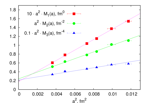
Figure 1: Scaling of the correlators ${\cal M}_{n}$, Eqs. (27), (28), (29), with diminishing lattice spacing. Lines represent the best fits according to Eq. (30).

What is even more important here is that the numerical data (30) is in perfect qualitative agreement with the assumption (11). Moreover, the actual numerical values of the coefficients $\alpha_{n}$, $\beta_{n}$ provide the self-consistency check of the ansatz (11). Indeed, considering Eq. (30) for $n=1$ and $n=2$ we obtain

$$\alpha_{1}\cdot\beta_{1} = \beta_{2}\,,$$ (31)

$$\sum\limits_{i<j}{\langle\lambda_{i}\lambda_{j}\rangle} = \alpha_{2}\,,$$

while the combination of $n=2$ and $n=3$ cases leads to

$$\beta_{3}~{}=~{}\beta_{1}\cdot\sum\limits_{i<j}{\langle\lambda_{i}\lambda_{j}\rangle}~{}=~{}\beta_{1}\cdot\alpha_{2}\,.$$ (32)

Evidently, Eqs. (31), (32) are highly non-trivial and their numerical validity would definitely signify the correctness of the ansatz (11). As far as the numerical values of the relevant coefficients are concerned, the outcome of the best fits according to Eq. (30) is

$$\begin{array}[]{rcrcrcr}a^{2}\cdot\alpha_{1}&=&11.8(3)\,,&&\beta_{1}&=&0.018(2)\,,\\ a^{4}\cdot\alpha_{2}&=&87(3)\,,&&a^{2}\cdot\beta_{2}&=&0.24(2)\,,\\ &&&&a^{4}\cdot\beta_{3}&=&2.1(2)\,.\end{array}$$ (33)

One can see that these numbers are in the perfect agreement with Eq. (31)

$$\frac{\alpha_{1}\cdot\beta_{1}}{\beta_{2}}~{}=~{}0.9(1)\,,$$ (34)

and are compatible with Eq. (32)

$$\frac{\beta_{1}\cdot\alpha_{2}}{\beta_{3}}~{}=~{}0.8(2)\,,$$ (35)

although the deviation from unity and numerical uncertainty is larger in the latter case.

The conclusion is that numerical data supports strongly the assumption (11) so that indeed the topology defining map $S^{4}\to{\mathrm{HP}^{1}}$ is likely to be highly asymmetric. One of the relevant eigenvalues is divergent in the continuum limit and seems to depend only on the ultraviolet cutoff. On the other hand, the remaining eigenvalues are sensitive solely to the infrared scale and show no divergences near the continuum limit.

Finally, we note that it is tempting to consider along the same lines the fourth order correlator ${\cal M}_{4}={\langle\prod\lambda_{\mu}\rangle}$ and then relate via Eq. (15) its spacing dependence with leading UV behavior of the topological density. In turns out that numerically ${\cal M}_{4}(a)$ is indeed compatible with (30), however, we refrain to rely on (15) at finite lattice spacing The point is that Eq. (15) is certainly valid in the limit $a\to 0$, provided that ${\cal M}_{4}$ stays constant in physical units. However, due to the suspected power divergence the corrections to Eq. (15) are difficult to estimate.

III.2 Topological Fluctuations at Various Scales

As was repeatedly stressed in Refs. Gubarev:2005rs ; Boyko:2005rb any discussion of the topological charge density within the lattice settings inevitably introduces a particular cutoff $\Lambda_{q}$ on the magnitude of the density so that $q(x)$ is equated to zero if $|q(x)|<\Lambda_{q}$. Indeed, the most straightforward argument here is that in the numerical simulations the density is always known with finite accuracy. Thus the numerical precision provides the finest possible cutoff which in physical units evidently scales like $\Lambda_{q}\propto a^{-4}$. Moreover, the introduction of (often implicit) finite $\Lambda_{q}$ is inherent to all studies of the gauge fields topology. For instance, the chiral fermions based topological density, which is given by the sum of Dirac eigenmodes $\psi_{\lambda}$ contributions, is usually either restricted to lowest modes, $\lambda<\Lambda\propto\Lambda_{QCD}$, or is considered for all modes available on the lattice, $\lambda\lesssim 1/a$. Therefore the actual problem is not the presence of the cut $\Lambda_{q}$, it is introduced always. The physically meaningful question is the spacing dependence $\Lambda_{q}=\Lambda_{q}(a)$ and the above examples illustrate two extreme cases $\Lambda_{q}\propto a^{-4}$ and $\Lambda_{q}\propto\Lambda^{4}_{QCD}$.

It is crucial that the scaling law $\Lambda_{q}(a)$ could be taken at will and we’re going to exploit this freedom to study the spacing dependence of the topological density. Indeed, if the characteristic topological density $\bar{q}$ stays constant in physical units then the volume density of points at which $|q(x)|>\Lambda_{q}$,

$$\rho(\Lambda_{q})=\frac{1}{V}\sum\limits_{x}\left\{\begin{array}[]{cc}1\,,&|q(x)|>\Lambda_{q}\\ 0\,,&\mbox{otherwise}\end{array}\right.\,,$$ (36)

should also be lattice spacing independent for $\Lambda_{q}\propto\Lambda^{4}_{QCD}$. Note that the lattice units had been used in (36) and that $\rho(\Lambda_{q})$ is dimensionless, positive, bounded $\rho(\Lambda_{q})\leq 1$ quantity, unrelated to the volumes $V_{\pm}$ discussed in section II.2. It is clear that the divergence $\bar{q}\sim a^{-\alpha}$ would result in the divergent behavior $\rho(\Lambda_{q})\sim a^{-\alpha}$ of the volume density for physical cut $\Lambda_{q}\propto\Lambda^{4}_{QCD}$, while $\rho(\Lambda_{q})$ is to be almost spacing independent for similarly divergent cut $\Lambda_{q}\propto\Lambda^{4}_{QCD}\cdot(a\,\Lambda_{QCD})^{-\alpha}$. Therefore the most straightforward way to analyze the spacing dependence of the characteristic topological density is to tune the scaling law $\Lambda_{q}(a)$ until the volume density $\rho(\Lambda_{q})$ becomes constant at various lattice resolutions.

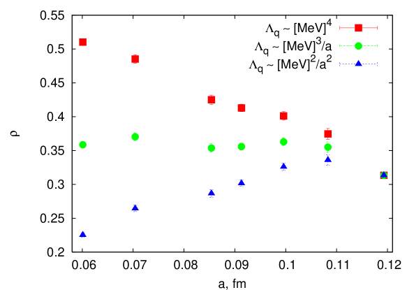
Figure 2: Volume density of points with $|q_{x}|>\Lambda_{q}$ as a function of lattice spacing at different $\Lambda_{q}$ scaling laws (37).

Unfortunately, this approach does not allow to investigate the dependence $\bar{q}(a)$ precisely. Indeed, on the lattice we could only probe a finite set of scaling laws $\Lambda_{q}(a)$, moreover the corresponding estimates of $\rho(\Lambda_{q})$ are always biased. However, it is crucial that the correct qualitative picture could easily be obtained this way. We performed the measurements of the volume density $\rho(\Lambda_{q})$ at various lattice spacings using three different scaling laws

$$\Lambda^{(n)}_{q}~{}\propto~{}\Lambda^{4}_{QCD}\cdot(a\,\Lambda_{QCD})^{-n}\,,\qquad n=0,1,2\,,$$ (37)

where the numerical coefficients were chosen in such a way that $\Lambda^{(n)}_{q}=[200\mathrm{~{}MeV}]^{4}$, $n=0,1,2$ at $a=0.1193\mathrm{~{}fm}$ (this particular choice is motivated below). The results of our measurements are presented on Fig. 2 from which it is clear that the volume density of points with $|q_{x}|>\Lambda^{(0)}_{q}=[200\mathrm{~{}MeV}]^{4}$ is rapidly rising with diminishing lattice spacing. Contrary to that the linearly divergent cut on the topological density, $\Lambda^{(1)}_{q}\sim 1/a$ results in the almost spacing independent volume density $\rho(\Lambda^{(1)}_{q})\approx 0.35$. On the other hand, once the quadratically divergent cut $\Lambda^{(2)}_{q}\sim 1/a^{2}$ is imposed the quantity $\rho(\Lambda^{(2)}_{q})$ diminishes almost linearly with vanishing lattice spacing and in the limit $a\to 0$ becomes compatible with zero. The conclusion is that the characteristic magnitude of the topological density is indeed singular in the continuum limit, the leading divergence is compatible with linear one

$$\bar{q}~{}\propto~{}\Lambda^{3}_{QCD}\,/\,a$$ (38)

and is in accord with theoretical expectations (15).

Let us discuss now the dimensionality of topological charge sign-coherent regions. Qualitatively the structure of topological fluctuations at various cuts $\Lambda_{q}$ is rather simple Gubarev:2005rs ; Boyko:2005rb . For utterly small values of $\Lambda_{q}$ there are typically only two large (percolating) regions of sign-coherent topological density, each of which occupies almost half of the lattice volume and carries rather large topological charge $Q_{\pm}$, Eq. (16). With rising cutoff the volume density of percolating regions diminishes, while the number of small sign-coherent lumps rapidly grows. Finally a sort of percolation transition happens at which the percolating regions cease to exist and become indistinguishable from the small lumps. After that point the volume distribution of sign-coherent regions become universal ($\Lambda_{q}$ independent) and is described by rather remarkable power law. However, the physics changes drastically at the lumps percolation transition. Namely, the string tension, associated with ${\mathrm{HP}^{1}}$ projected fields and which accounts for the full $SU(2)$ string tension in the continuum limit, vanishes. Already from this observation we expect that the most physically important topological fluctuations are represented by the largest (at given cutoff $\Lambda_{q}$) lumps in topological density and it is natural to focus exclusively on their dimensionality. Note that the actual values of the cuts (37) were taken to be always below the lumps percolation transition in the whole range of lattice spacings considered.

However, at any fixed cutoff $\Lambda_{q}$ the structure of the lumps is very complicated and their dimension is, in fact, not a well defined concept. Indeed, the notion of dimensionality makes sense only as a scaling relation since at any fixed lattice spacing the lumps occupy some finite fraction of the volume. Actually the situation is much worse since the very definition of the lumps require introduction of the cutoff $\Lambda_{q}$, the spacing dependence of which is not fixed. Moreover, admitting the lower dimensionality of sign-coherent regions, their volume fraction is not obliged to be finite in the continuum limit, hence even the spacing dependence of lumps localization degree (which might be expressed in terms of inverse participation ratio or similar quantities) would not reveal their dimensionality.

It is clear that the crucial obstacle in lumps dimensionality definition is the necessity to impose the cutoff on the topological density. The concept of the dimensionality of topological fluctuations would become unambiguous provided that we could get rid of explicit $\Lambda_{q}$ and hence reject the language of the lumps. This program is implemented in section III.4. However before going into details let us study the divergence (38) more quantitatively and consider the topological density correlation function.

III.3 $\langle q_{0}q_{x}\rangle$ Correlation Function

It is was discussed in brief in section II.1 that considering the magnitude of the characteristic topological density defined by $\bar{q}^{2}\equiv\lim_{x\to 0}{\langle q_{0}q_{x}\rangle}$ one has to prove that $\bar{q}$ indeed makes sense and is not equivalent to the contact term inherent to the perturbation theory. It was stated without proof that this is the case for ${\mathrm{HP}^{1}}$-based topological density. In this section we present the corresponding data and investigate the correlation function ${\langle q_{0}q_{x}\rangle}$. Note that the correlator ${\langle q_{0}q_{x}\rangle}$ is known to be negative at any non-vanishing distance Seiler:2001je provided that the definition of the topological density is local (see also Refs. Ilgenfritz:2005hh ; Horvath:2005cv ; Horvath:2005rv for discussions). However, the requirement of locality is a priori violated in ${\mathrm{HP}^{1}}$ embedding approach so that ${\langle q_{0}q_{x}\rangle}$, $|x|\neq 0$ is not obliged to be negative. We could only hope that the intrinsic non-locality is not so violent and extends up to some distance $R_{0}$ fixed in physical units. Note that this expectation is not completely groundless. Indeed, many non-perturbative observables, defined via ${\mathrm{HP}^{1}}$ projection and studied in Refs. Gubarev:2005rs ; Boyko:2005rb , do not reveal any pathology and reproduce, in fact, the corresponding results in the full theory. Actually the degree of non-locality of ${\mathrm{HP}^{1}}$ method could be estimated from the behavior of heavy quark potential measured at $a=0.0601\mathrm{~{}fm}$ in Boyko:2005rb and it turns out to be of order $R_{0}\lesssim 0.2\mathrm{~{}fm}$. On the other hand, the investigation of ${\langle q_{0}q_{x}\rangle}$ correlation function allows to find $R_{0}$ rather precisely and check its scaling properties.

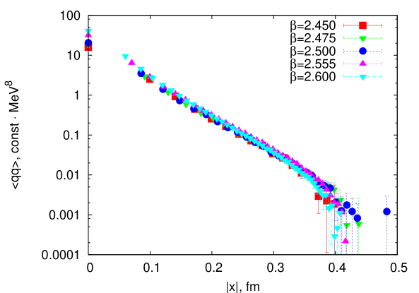
Figure 3: Positive core of topological density correlation function ${\langle q_{0}q_{x}\rangle}$ at distances $|x|<R_{0}\approx 0.4\mathrm{~{}fm}$.

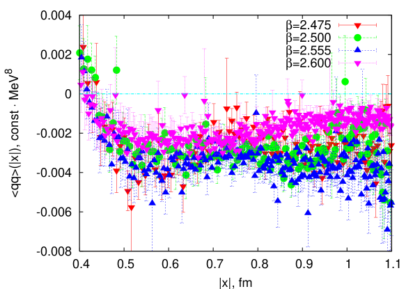
Figure 4: Negative part of the correlation function ${\langle q_{0}q_{x}\rangle}$ at distances $|x|\geq R_{0}=0.4\mathrm{~{}fm}$ at various lattice spacings.

Generically we expect that the correlator ${\langle q_{0}q_{x}\rangle}$ is to be positive up to the distance $R_{0}$ and then should become negative provided that $R_{0}$ is finite. Remarkably enough these expectations are precisely confirmed by the measurements. The positive core of ${\langle q_{0}q_{x}\rangle}$ correlation function at small $|x|$ is presented in physical units on Fig. 3. It is apparent that the points at various spacings are well described by the exponential $|x|$-dependence

$${\langle q_{0}q_{x}\rangle}~{}\propto~{}e^{-|x|/R_{qq}}\,,\qquad|x|\lesssim R_{0}\,.$$ (39)

Note that due to the logarithmic scale used on this plot the data sets are terminating at the same physical distance, for larger $|x|$ the correlation function becomes negative. Therefore the degree of non-locality inherent to ${\mathrm{HP}^{1}}$ embedding method is given roughly by

$$R_{0}~{}\lesssim~{}0.4\mathrm{~{}fm}$$ (40)

and is indeed constant in physical units as is evident from Fig. 3. Moreover, the almost perfect scaling of various data sets indicates once again that ${\mathrm{HP}^{1}}$ projected fields do not contain any trace of the perturbation theory. Indeed, the mixture with perturbative contributions would lead to notable $\sim-1/|x|^{8}$ terms and would result in rather abrupt deviation from the exponential behavior. On the other hand, at large distances, $|x|\gtrsim R_{0}$, the correlation function ${\langle q_{0}q_{x}\rangle}$ indeed becomes negative as is illustrated on Fig. 4. It is important that the negative part of ${\langle q_{0}q_{x}\rangle}$ correlator does not show any singularity in the limit $a\to 0$, in particular, it has nothing to do with usual perturbative dependence.

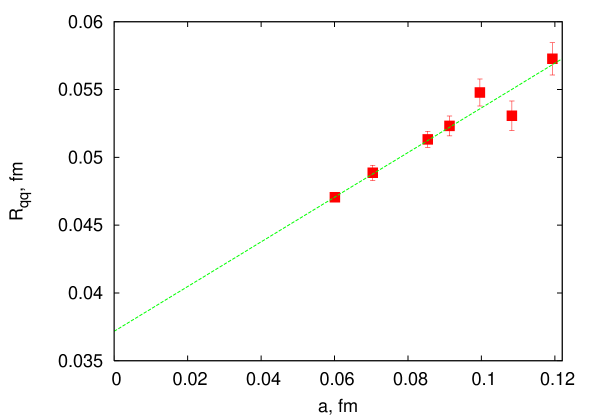
Figure 5: Correlation length $R_{qq}$, Eq. (39), as a function of lattice spacing. Line represents the best linear fit.

Let us consider the scaling properties of the correlation length $R_{qq}$, Eq. (39). As might be expected already from Fig. 3, $R_{qq}$ decreases with diminishing lattice spacing. In more details the dependence $R_{qq}(a)$ is presented on Fig. 5, from which it is apparent that the correlation length is likely to be linear function of $a$ with rather small continuum value

$$R_{qq}~{}=~{}0.037(1)\mathrm{~{}fm}\,.$$ (41)

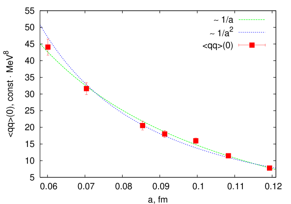
Figure 6: The mean squared topological density ${\langle q^{2}\rangle}$ as a function of lattice spacing. Curves represent the best power law fits, Eq. (43).

As is apparent from the above presentation, the short distance behavior of ${\langle q_{0}q_{x}\rangle}$ correlation function is definitely exempt from the perturbative uncertainties and in the limit $|x|\to 0$ the characteristic topological density

$$\bar{q}^{2}={\langle q^{2}\rangle}=\lim_{|x|\to 0}{\langle q_{0}q_{x}\rangle}$$ (42)

has nothing to do with contact terms inherent to the usual approaches. Therefore let us consider the dependence of $\bar{q}$ upon the ultraviolet cutoff. The results of our measurements are presented on Fig. 6 from which it is clear that ${\mathrm{HP}^{1}}$-based characteristic topological density still diverges in the continuum limit. However, this divergence has nothing in common with perturbatively expected $O(a^{-8})$ behavior, in fact, it is much weaker and is compatible only with linear or quadratic dependence

$${\langle q^{2}\rangle}~{}=~{}b_{n}~{}+~{}c_{n}\cdot a^{-n}\,,\qquad n=1,2\,.$$ (43)

Unfortunately, our data points do not distinguish these power laws and are adequately described by either linear ($\chi^{2}_{n=1}=0.9$) or quadratic ($\chi^{2}_{n=2}=1.5$) one. Nevertheless, the ultraviolet divergence of characteristic topological density $\bar{q}\sim a^{-\alpha}$ within the ${\mathrm{HP}^{1}}$ embedding method could be considered as firmly established. Moreover, we are confident that the corresponding power exponent is close to unity, $\alpha\lesssim 1$, and is in accord with theoretical expectations (15) and the estimate (38) obtained earlier.

III.4 Dimensionality of Topological Charge Fluctuations

III.4.1 Biased Random Walk Model and the Choice of Parameters

In this section we introduce the model, which allows to investigate directly the dimensionality of the relevant topological fluctuations. Although the resulting method is not entirely rigorous, its ambiguity reduces to only one free parameter, the choice of which we thoroughly discuss. Generically the idea is to consider some dynamical system the evolution of which is sensitive to the dimensionality of the ambient space. Then if we embed somehow this system into the topological density background, its evolution will reveal the effective number of available dimensions, which is to be naturally associated with the dimensionality of the relevant topological fluctuations. The simplest dynamical system of this sort could be constructed on the top of usual diffusion equation, which in turn is equivalent to the model of random walks. Then the dependence upon the external environment could be introduced by making the hopping probabilities to be the local functions of the ambient space characteristics; the models of this sort are known as biased random walks. Correspondingly, the effective dimensionality $D$ as is seen by biased random walkers is referred to as diffusion dimension. The purpose of this section is to precisely formulate and investigate this approach.

We start from the observation that the introduction of the cutoff $\Lambda_{q}$ on the topological density (see section III.2) was aimed solely to separate the inevitably present noise (utterly small values of $q_{x}$) from the relevant fluctuations, which are associated with relatively large values of $q_{x}$. Although the choice of particular $\Lambda_{q}$ indeed makes the notion of ’small’ and ’large’ well defined, the geometry of the resulting lumps in topological density strongly depends upon the cut. It is apparent that the weak point here is sharpness of the dimension four cut, it would be much advantageous to remove the small topological density regions softly, making the lumps geometry much more robust with respect to the parameters involved. It turns out that slightly modified diffusion model is indeed suitable to achieve this. Namely, we propose to modify the diffusion equation by allowing the random walk to hop towards the regions of higher topological density with larger probability. In the language of the diffusion equation, which describes the propagation of heat, this amounts to the introduction of space-time dependent diffusion coefficient (thermal conductivity), which vanishes in the regions of small topological density, and hence heat is allowed to spread only within the domains of large $|q_{x}|$. Then the decay rate of the initial heat pulse, which is the same as the return probability for corresponding biased random walk, essentially reflects the number of available dimensions within the topological fluctuations and hence is to be identified with their dimensionality.

In fact, this general idea fixes almost uniquely the random walk model which we would like to investigate. It is convenient to start directly from the microscopic rules of the biased random walk, which require that the probability $p_{x,x+\mu}$ to hop from point $x$ to the neighboring site $x+\mu$ is monotonically rising scale free function of the topological density magnitude at $x+\mu$

$$p_{x,x+\mu}=\frac{|q_{x+\mu}|^{\gamma}}{\sum_{\mu}(|q_{x+\mu}|^{\gamma}+|q_{x-\mu}|^{\gamma})}\,,$$ (44)

where the power exponent $\gamma>0$ could not be fixed a priori and remains free parameter of the model. Note that in this section we exclusively consider the local magnitude $|q_{x}|$ of the topological density; to lighten the notations the corresponding modulus sign will be omitted. From Eq. (44) it is straightforward to obtain the continuum diffusion-like equation, which determines the probability $P(t,x)$ to reach the point $x$ during the proper time interval $t$ provided that at $t=0$ walker starts at $x=0$ (see, e.g., Ref. Itzykson )

$$\partial_{t}\Phi~{}=~{}\frac{1}{8}\,q^{-2\gamma}\,\partial_{x}\left[\,q^{2\gamma}\,\partial_{x}\Phi\right]\,,$$ (45)

$$\Phi(t,x)\equiv P(t,x)/q^{2\gamma}(x)\,,$$

where the initial condition is $P(0,x)=\delta(x)$. However, Eq. (45) is not yet the usual diffusion equation, in particular, the decay rate of the initial perturbation (return probability in the random walk language) is not guaranteed to be $P(t,0)\propto t^{-D/2}$. To get the correct interpretation of (45) we introduce new coordinates $\zeta(x)$ according to

$$\partial\zeta^{\mu}/\partial x^{\nu}~{}=~{}q^{2\gamma}\cdot\delta^{\mu}_{\nu}\,.$$ (46)

In the particular case of one dimensional problem (46) allows explicit solution $\zeta(x)=\int^{x}q^{2\gamma}$, where the lower integration limit is taken at arbitrary fixed point. It is important that $\zeta$ is a single valued function of $x$ almost everywhere, moreover, its range is determined by the magnitude of the topological density. Indeed, the regions of utterly small $|q_{x}|$ are squeezed to almost one point by the map (46) regardless how large these regions were in $x$ space. It is crucial that the term ’small’ above obtains unambiguous and physically correct meaning of relative smallness since only the relative variation of the topological density does matter. Indeed, Eq. (45) is evidently scale invariant under $q\to\lambda q$ and is equivalent to usual diffusion equation for everywhere constant $q_{x}$. In terms of new coordinates Eq. (45) takes the standard form

$$\partial_{t}\Phi~{}=~{}\frac{1}{8}\,\partial_{\zeta}\left[\,q^{4\gamma}\,\partial_{\zeta}\Phi\right]\,.$$ (47)

We conclude therefore that the diffusion process (44), (45), (47) takes place in the regions of relatively large topological density and hence should reflect properly the dimensionality of underlying topological background. Moreover, the decay rate of the initial perturbation is given by

$$\Phi(t,0)~{}\propto~{}t^{-D(\gamma)/2}\,,$$ (48)

where $D(\gamma)$ is the diffusion dimension of the topological fluctuations and we have explicitly indicated that the dimension defined this way depends non-trivially upon yet not fixed parameter $\gamma$ to be discussed next.

The non-triviality of the dependence $D(\gamma)$ is evident since in the limit $\gamma\to 0$ the model (44), (45) reduces to standard unbiased random walk with

$$D(\gamma\to 0)~{}=~{}4\,,$$ (49)

while at $\gamma\to\infty$ the microscopic probability (44) allows the hopping only towards largest neighboring $|q_{x}|$. Hence the walker is trapped eventually at the local maxima of topological density distribution and

$$D(\gamma\to\infty)~{}=~{}0\,,$$ (50)

regardless of the background. Already from this observation it is apparent that without an additional physical input the model (44), (45) would be essentially useless since at various $\gamma$ it reflects, in fact, different properties of the underlying background. For instance, the limiting behavior (49) implies that the topological density distribution is such that $q_{x}\equiv 0$ only on measure zero set, while (50) is valid generically, provided $q_{x}$ is not identically constant. Therefore the actual problem is not the arbitrariness of $\gamma$ parameter, but rather yet not posed physical question we’re trying to investigate.

In order to gain a physical insight it is crucial to retain the qualitative picture of vacuum topological excitations outlined in section III.2. It was argued that physically most important fluctuations are associated with percolating sign-coherent regions, the ultimate qualitative properties of which are the significant internal topological density and extremely large linear extent. It goes without saying that we are interested precisely in the geometry of these sign-coherent domains. However, the percolating lumps are not equivalent to just the regions of largest topological density as is revealed by the percolation transition eventually appearing with rising $\Lambda_{q}$ cutoff. Even at large $\Lambda_{q}$ one finds individual ’hot spots’ of small but non-vanishing volume which indeed possess the largest topological density. Consider now the decay rate of the initial heat pulse in the model (45) at large but finite $\gamma$, so that the effective thermal conductivity is non-zero only within the topological density hot spots. Evidently, in this regime the equilibration time $t_{eq}$ is finite and is dictated by the typical size of the hot spots being much smaller than the squared lattice size $L$

$$t_{eq}\ll L^{2}\quad\mbox{for}\quad\gamma\gg\gamma^{*}$$ (51)

(the definition of $\gamma^{*}$ will become clear in the moment). Note that the distinct feature of this regime is that the double logarithmic plot of $\Phi(t,0)$ significantly bends upwards at $t_{eq}$ and therefore we expect generically that

$$\gamma>\gamma^{*}\,:\quad\frac{\partial^{2}\ln\Phi(t,0)}{\partial(\ln t)^{2}}>0\,,$$ (52)

reflecting, in particular, the drop in the effective thermal conductivity outside the hot spots. Evidently, at these $\gamma$ values we are not probing the percolating lumps geometry, the random walks are confined within the regions of largest topological density.

Let us now gradually diminish the $\gamma$ parameter. The positive jump in the logarithmic derivative $\partial\ln\Phi/\partial\ln t$, the location of which we still denote by $t_{eq}$, would become smaller respecting the diminishing difference of thermal conductivities inside and outside the hot spots. Note that neither of the corresponding diffusion dimensions at $t\gtrless t_{eq}$ could be identified with the dimensionality of sign-coherent regions since the random walks are still too sensitive to the local irregularities of topological density even within the coherent domains. It might happen that at the particular value $\gamma=\gamma^{*}$ the double logarithmic plot of $\Phi(t,0)$ degenerates into the straight line so that $t_{eq}\approx L^{2}$ and

$$\gamma=\gamma^{*}\,:\quad\frac{\partial^{2}\ln\Phi(t,0)}{\partial(\ln t)^{2}}=0\,,\quad t\lesssim L^{2}\,.$$ (53)

Note that at this point the only relevant dimensional parameter is the lattice size. Therefore the model becomes essentially scale free and its dynamics in the vicinity of $\gamma^{*}$ is reminiscent to the disorder driven conductor-insulator transition of condensed matter systems. It is crucial that at the critical point $\gamma=\gamma^{*}$ the heat starts to propagate with constant rate over largest available distances, but since the thermal conductivity is significant only within the lumps, the heat transfer goes through the percolating sing-coherent regions. In turn the condition (53) implies that local inhomogeneity of the topological density within the percolating lumps is inessential. Therefore it seems that only at the critical point (53) we indeed could obtain a consistent reflection of the relevant topological fluctuations in the biased random walks model.

The existence of at least one critical value, $\gamma^{*}=0$, follows from (49), but it is trivial one and surely exists for arbitrary background $q_{x}$. However, it is crucial that the above qualitative picture of vacuum topological fluctuations hints on the existence of non-trivial critical coupling $\gamma^{*}>0$, which could arise entirely due to the low-dimensional long-range order present in the topological density distribution. For suppose that the topological charge sign-coherent regions are indeed lower dimensional objects possessing relatively large uniform topological density and extending through all the volume. Then at the particular $\gamma=\gamma^{*}$ the effective thermal conductivity would be non-zero only within the percolating regions, the lower dimensionality of which forbids the appearance of an additional scale in the heat propagation problem. Thus at this point the random walks model indeed contains no dimensional parameter apart from the lattice size and Eq. (48) is fulfilled, while the corresponding diffusion dimension is to be identified naturally with the dimension of sign-coherent regions. Note that the lower dimensionality is crucial here, for regions of finite thickness the critical point (53) does not exists. In fact, the analogous but reversed argumentation could also be given, namely, the appearance of non-trivial critical point (53) signifies the presence of lower dimensional long-range order in the topological density background.

Note that the restriction to sign-coherent regions is automatic in our approach. Indeed, as far as the model (45) is concerned, it was considered in the continuum limit assuming differentiability of $q_{x}$. Hence the domains $q_{x}\gtrless 0$ are separated by regions with vanishing thermal conductivity. On the lattice the situation is more involved, but since the ${\mathrm{HP}^{1}}$-based topological density is definitely exempt from perturbative contributions we could be almost confident that the same argumentation applies.

To summarize, the proposed biased random walk model seems to be efficient to investigate the structure of percolating topological density regions only at the critical points, at which its dynamics becomes effectively scale free. We argued that the qualitative picture of the relevant topological fluctuations obtained earlier suggests the existence of non-trivial critical point, at which the diffusion dimension is to be identified naturally with the percolating regions dimensionality.

III.4.2 Diffusion Dimension of Percolating Lumps

Prior to presenting the results of our measurements let us discuss the lattice specific features of the above biased random walk model, which complicate the numerical evaluation of the percolating lumps dimensionality. For any particular $\gamma$ value the solution of Eq. (45) could be constructed straightforwardly by implementing the random walk process, the rules of which are completely specified by (44). The only subtlety here is the choice of the random walk starting point. Indeed, to improve the statistics it is desirable to consider

$$\Phi(t,0)=\frac{\int d\zeta_{0}\,\Phi(0,\zeta_{0};t,\zeta_{0})}{\int d\zeta_{0}}=$$ (54)

$$=\int dx_{0}\,\Phi(0,x_{0};t,x_{0})\,\frac{q^{8\gamma}(x_{0})}{\int q^{8\gamma}}\,,$$

where $\Phi(0,x_{0};t,x)$ is the probability to reach the point $x$ during the proper time $t$ starting at $x_{0}$. Eq. (54) means that the random walk starting point in $x$ space is to be taken with probability $\propto q^{8\gamma}$.

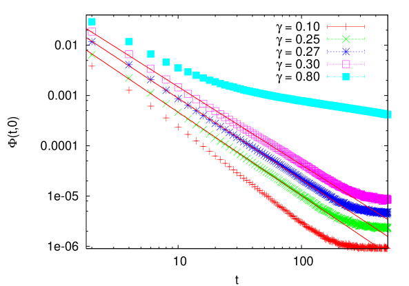
Figure 7: Return probability of biased random walk $\Phi(t,0)$, Eqs. (44, 45), at different $\gamma$ values for $\beta=2.500$ data set. Solid lines are the best fits of $\gamma=\{0.25,0.27,0.30\}$ data points to Eq. (48), fitting range is $t<100]$.

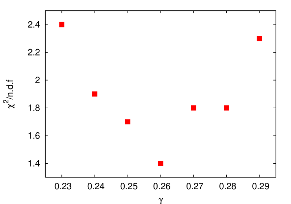
Figure 8: Quality of the power law fits of the return probability $\Phi(t,0)$ to Eq. (48) in the range $t<100$ at various $\gamma$ values. Measurements were performed on $\beta=2.500$ data set.

Therefore the crucial problem is how to find the relevant $\gamma^{*}$ value numerically and estimate the accuracy of its determination. For any fixed $\gamma$ we measured $\Phi(t,0)$ by first taking some random starting point, chosen with $\propto q^{8\gamma}$ probability, and considering in accord with (44) the walk of total length $8\cdot 10^{3}$. Then the quantity $\Phi(t,x)=P(t,x)/q^{2}(x)$ was constructed for each random walk and averaged with respect to $\approx V/2$ different starting points per configuration ($V$ is the lattice volume). We checked that the statistics is large enough so that our results do not change if more random walks are considered. Fig. 7 represents the double logarithmic plot of the quantity $\Phi(t,0)$ obtained on our $\beta=2.500$ set at three close $\gamma$ values, $\gamma=\{0.25,0.27,0.30\}$, as well as the same quantity measured at $\gamma=0.1$ and $\gamma=0.8$. Note that for readability reasons different graphs are slightly shifted with respect to each other. As far as the data points at $\gamma=0.1$ and $\gamma=0.8$ are concerned they definitely correspond to the regimes $\gamma\ll\gamma^{*}$ and $\gamma\gg\gamma^{*}$ respectively. Indeed, the first graph significantly bends downwards at $t\approx 10\div 20$ in apparent disagreement with both Eq. (52) and Eq. (53). However, it is demonstrated below that negative second logarithmic derivative of $\Phi(t,0)$ is a generic feature of the diffusion model in random environment. Note that at $\gamma=0.1$ the system indeed equilibrates eventually at $t_{eq}$ of order few hundred, which is similar to squared size of the lattice used in this calculation. On the other hand, at $\gamma=0.8$ the system starts to equilibrate at $t_{eq}\approx 20\ll L^{2}$ and the corresponding graph has positive second derivative in accord with Eq. (52).

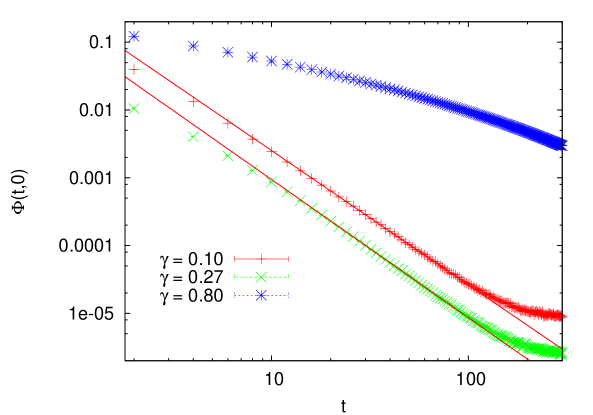
Figure 9: Return probability $\Phi(t,0)$, Eqs. (44, 45), calculated on $\beta=2.500$ data set with random permutation of topological density records on each configuration.

$\beta$ 2.4000 2.4273 2.4500 2.4750 2.5000 2.5550 2.6000 $\gamma^{*}$ 0.27(3) 0.27(3) 0.27(4) 0.27(4) 0.26(2) 0.27(3) 0.28(3)

Table 2: Estimated $\gamma^{*}$ values for various data sets from Table 1.

The inspection of the intermediate $\gamma$ values reveals that $\gamma=0.25$ data points essentially lie on one single line, while the data set at $\gamma=0.30$ seems to deviate upwards from linear dependence. Note that the consideration of $\gamma=0.27$ points are rather inconclusive, apparently the data just begins to bend aside the pure power law. Therefore the relevant $\gamma^{*}$ value seems to be located around $\gamma^{*}\approx 0.25$. We could estimate $\gamma^{*}$ more rigorously by considering the quality of power law (48) fits at different $\gamma$. We fitted our data to Eq. (48) in the range $t<100$, the resulting $\chi^{2}/\mathrm{n.d.f.}$ values are presented on Fig. 8. It is apparent from this figure that fits favor the critical value $\gamma^{*}=0.26(2)$, where rather conservative errors coming from Fig. 8 are quoted.

In order to convince the reader that graphs on Fig. 7 are indeed directly related to the underlying geometry of topological fluctuations, let us consider the same model (44), (45) with the same parameters, but in the genuinely random external environment. Such a background, which is the ’nearest’ to one on Fig. 7, could be obtained by random permutation of the topological density records on each configuration. We did this with our $\beta=2.500$ data set and then performed the identical measurements of $\Phi(t,0)$ at $\gamma=\{0.10,0.27,0.80\}$. The corresponding double logarithmic plots are presented on Fig. 9 and differ violently from that on Fig. 7. The most crucial observation is that the second derivative for all graphs stays negative implying that the reasoning of section III.4.1 is inapplicable for randomly permuted topological density. Of course, this is not surprising since all the coherent structures are gone in the present case. The only limit in which the second logarithmic derivative of $\Phi(t,0)$ vanishes is given either by Eq. (49), $D=4$, or Eq. (50), $D=0$. We conclude therefore that without random permutations the non-trivial critical point $\gamma^{*}$ arises most likely due to the presence of long-range order in the topological density.

We performed the measurements of the relevant $\gamma^{*}$ values for all our data sets listed in Table 1. It goes without saying that indeed in each case the biased random walk return probability at $\gamma=\gamma^{*}$ strictly obeys the power law (48). The resulting estimations of corresponding $\gamma^{*}$ values are summarized in Table 2. It is remarkable that the estimates of $\gamma^{*}$ appear to be spacing independent well within the quoted numerical uncertainties. It is true that the presented errors might be overestimated, however, we are confident that $\gamma^{*}(a)$ dependence could not be revealed by the above method. Apparently this is due to the fact that $\gamma$ parameter is dimensionless so that the violent power dependence on the lattice spacing is unlikely to appear.

Once the relevant $\gamma^{*}$ values are determined for every our data set it is straightforward to estimate the dimensionality of sign-coherent percolating regions of the topological density. By construction the corresponding fits to Eq. (48) are practically perfect for every $\beta$ so that we do not present full details of the fitting procedure. The point which should be discussed, however, is $D(\gamma^{*})$ error estimation. In fact, the uncertainty coming from the fits to Eq. (48) is negligible compared to the ambiguity in $\gamma^{*}$ values. Therefore the errors in $D(\gamma^{*})$ were obtained by repeating the fits to Eq. (48) at minimal and maximal $\gamma^{*}$ within the corresponding error bands. Finally, we note that all fits were performed in the range $t<100$.

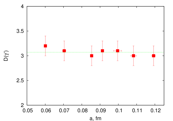
Figure 10: Diffusion dimensions $D(\gamma^{*})$, Eqs. (44), (45), (48), at various lattice spacings. Line represents the fit to the constant behavior.

The dimensionality of percolating sign-coherent regions of topological density measured with the above procedure at various lattice spacings is summarized on Fig. 10. Remarkably enough the diffusion dimension $D(\gamma^{*})$ seems to be almost independent upon the lattice resolution well within the uncertainties. Its continuum value could be estimated from fit to constant behavior, which indicates in turn that $D(\gamma^{*})$ is definitely smaller than 4. Instead the numerical data suggests strongly that the diffusion dimension of the relevant topological fluctuations is

$$D~{}\equiv~{}D(\gamma^{*})~{}=~{}3.07(3)\,,$$ (55)

which seems to be in full agreement with their proposed three dimensional structure. Eq. (55) is in agreement with both theoretical expectations and experimental data on the topological density. What is still to be considered is the internal consistency of the scenario outlined in our paper, which is expressed by Eqs. (21), (23); this is the subject of the next section. Note, however, that the diffusion dimension is not the only definition of the dimensionality. It is still worth to confirm Eq. (55) with other methods.

III.5 Consistency Check

As was discussed in section II.2 the crucial equations which relate the divergence of characteristic topological density $\bar{q}$ and the dimensionality $D$ of the relevant topological fluctuations are

$${\langle Q_{+}Q_{-}\rangle}={\langle Q_{+}\rangle}{\langle Q_{-}\rangle}\,,$$ (56)

$${\langle Q^{2}_{\pm}\rangle}-{\langle Q_{\pm}\rangle}^{2}\propto{\langle Q_{\pm}\rangle}\,,$$ (57)

where the charges $Q_{\pm}$ are to be calculated without any cutoff $\Lambda_{q}$ imposed. Moreover, the spacing independence of (56), (57) (if confirmed by the data) allows to put rather stringent restrictions on both $\bar{q}$ and $D$. As far as the lattice measurements are concerned, Fig. 11 represents the ratios

$${\cal A}(Q_{\pm})=\frac{{\langle Q_{+}Q_{-}\rangle}}{{\langle Q_{+}\rangle}{\langle Q_{-}\rangle}} \mbox{(circles)}\,,$$ (58)

$${\cal B}(Q_{\pm})=\frac{{\langle Q^{2}_{\pm}\rangle}-{\langle Q_{\pm}\rangle}^{2}}{{\langle Q_{\pm}\rangle}} \mbox{(squares)}\,,$$

as a functions of lattice spacing, where to improve the statistics the generic equalities ${\langle Q^{2}_{+}\rangle}={\langle Q^{2}_{-}\rangle}$, ${\langle Q_{+}\rangle}={\langle Q_{-}\rangle}$ were used in calculation of ${\cal B}(Q_{\pm})$. As is evident from that figure Eq. (56) is satisfied identically in the whole range of considered spacings while the proportionality coefficient entering Eq. (57) does not depend upon the lattice resolution well within numerical errors. Therefore the validity of Eq. (25) is firmly established. Let us summarize the emerging qualitative picture of vacuum topological fluctuations which arises from the numerical data restricted by (25).

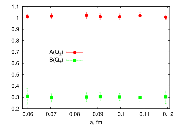
Figure 11: Fluctuations of the topological charges $Q_{\pm}$ at various lattice spacings. Circles: spacing (in)dependence of the ratio ${\cal A}(Q_{\pm})$, Eq. (58); squares: the magnitude of $Q_{\pm}$ relative fluctuations characterized by ${\cal B}(Q_{\pm})$, Eq. (58).

It is apparent that the most confidential data is available for the characteristic topological density. The theoretical arguments based on the existence of the quadratic correction to the gluon condensate as well as the obtained numerical data suggest strongly that the topological density is divergent at most linearly in the continuum limit

$$\bar{q}~{}\sim~{}a^{-\alpha}\,,\qquad\alpha\lesssim 1\,.$$ (59)

On the other hand, the dimensionality of topological fluctuations is still not firmly established and is plagued by theoretical uncertainties. Various estimations made both in this paper and in the literature Horvath:2005rv ; Aubin:2004mp ; Ilgenfritz:2005hh ; Horvath:2005cv ; Gubarev:2005jm ; Zakharov:2006vt suggest that it is of order three

$$\mathrm{dim}[V_{\pm}]~{}\approx~{}3\,.$$ (60)

It is remarkable that Eqs. (59), (60) overlap only at one point consistent with Eq. (25)

$$\alpha~{}=~{}1\,,\qquad\mathrm{dim}[V_{\pm}]~{}=~{}3\,.$$ (61)

Given that Eqs. (56), (57) are fulfilled with amazingly high accuracy we are forced to the conclusion that (61) is the only values consistent with both theoretical considerations and numerical data.

IV Conclusions

In this paper we further developed the $SU(2)$ gauge fields topology investigation method, based on the embedding of ${\mathrm{HP}^{1}}$ $\sigma$-model into the given gauge background Gubarev:2005rs ; Boyko:2005rb . Our prime purpose was to exploit the remarkable properties of ${\mathrm{HP}^{1}}$ projected fields found in Boyko:2005rb , namely, the factual absence of leading perturbative divergences and simultaneous existence of non-trivial quadratic power correction to the gluon condensate. It is clear that these striking features of the projected fields are to be encoded into the local structure of the topology defining map $S^{4}\to{\mathrm{HP}^{1}}$ and hence should be reflected in the corresponding topological density. The extended analysis of leading power corrections performed in this paper allows to conclude that the topological density is likely to be linearly divergent in the continuum limit. Note that this divergence has nothing to do with short distance perturbative singularities and is much weaker. The divergence of the topological density by itself is almost academical problem since it is not directly observable. However, combined with the requirement of ultraviolet finiteness of topological susceptibility it leads to rather dramatic consequences for the geometry of relevant topological fluctuations. Namely, we argued that the topological charge is to be concentrated in three-dimensional submanifolds of four-dimensional Euclidean space. This is the only conclusion compatible with physical topological susceptibility, numerically established pattern of power corrections and which does not necessitates explicit fine tuning of the Yang-Mills theory at UV scale. Moreover, the fine tuning assumption is testable and if it does not happen, then one could derive rather stringent relation between the divergence of the topological density and the dimensionality of submanifolds, which support the most of the topological charge. Note, however, that the lower dimensionality of topological fluctuations could also be considered as a sort of fine tuning, in which the explicit powers of UV cutoff are traded for unusual geometric properties. Qualitatively our results are in accord with modern trends in the literature, which discuss the lower dimensionality of physically relevant vacuum fluctuations Kovalenko:2005zx ; Gubarev:2002ek and, in particular, of the topological density sign-coherent regions Horvath:2005rv ; Aubin:2004mp ; Ilgenfritz:2005hh ; Horvath:2005cv ; Gubarev:2005jm ; Zakharov:2006vt ; Kovalenko:2005rz .

The actual experimental verification of this scenario turned out to be rather intricate both conceptually and technically; we believe that all these problems were adequately addressed in our paper. The technical achievement is the development of fast and rather precise numerical algorithm of topological density evaluation, which allowed us to investigate the problem on the convincing statistical level. While the UV behavior of the topological density could be studied directly, the dimensionality of relevant topological fluctuations is much more involved problem, which consists essentially in physical interpretation of the term “relevant” above. We argued that the natural approach is to embed a dynamical system into the topological density background, the evolution of which is sensitive to the dimensionality of ambient space. The simplest system of this sort could be constructed on the top of usual random walk model and depends upon one dimensionless parameter. Then the phase structure of the system and location of its critical-like points is ultimately related to the long-range properties of the underlying background and, in particular, to the dimensionality of sign-coherent topological regions.

As far as the results of numerical experiments are concerned, our data show unambiguously that non-perturbatively defined characteristic topological density is divergent in the continuum limit. Moreover, we were able to obtain the upper bound on its leading spacing dependence. At the same time, the dimensionality $D$ of the relevant topological fluctuations was shown to be decidedly less than four and is compatible with $D=3$. Here the assumed absence of the fine tuning becomes crucial and we showed that it indeed does not happen. Instead the topological charges associated with sign-coherent regions fluctuate independently. We conclude therefore that the only possibility to satisfy all the restrictions is to have linearly divergent topological density distributed in three-dimensional domains.

Appendix

Here we describe in details the numerical algorithm used in this paper to calculate the topological charge density. The general formulation of the problem could be found in Refs. Gubarev:2005rs ; Boyko:2005rb . Essentially it reduces to the evaluation of the volume $V(T)$ of 4-dimensional spherical tetrahedron $T$ embedded into $S^{4}$ with vertices $n^{A}_{i}$ given in terms of five $i=0,...,4$ unit five-dimensional $A=0,...,4$ vectors, $(\vec{n}_{i})^{2}=1$.

It is clear that for near vanishing $V(T)$ the volume is given by $V(T)=\mathrm{det}_{Ai}[n^{A}_{i}]$. Thus the volume of finite tetrahedron could be found by triangulating it into the set of small tetrahedra and summing up the infinitesimal volumes. In fact, our method works recursively until the determinant estimation of the volume of input tetrahedron is larger than $10^{-6}$; this way we indeed obtain the optimal performance. However, the determinant-based volume estimation is reliable and uniform only if the angles between all input vertices are small enough, e.g. $(\vec{n}_{i},\vec{n}_{j})>0$. In this case it suffices to place new triangulation vertex at $\vec{m}\propto\sum_{i}\vec{n}_{i}$ and complete the recursion cycle. However, this procedure must be modified if there are at least two input vertices $i$ and $j$ for which $(\vec{n}_{i},\vec{n}_{j})<0$. Indeed, in this case the above recursions converge non-uniformly and eventually lead to almost degenerate tetrahedra with large volume but still almost vanishing determinant. The needed modification is to take the new vertex at $\vec{m}\propto\vec{n}_{i}+\vec{n}_{j}$ which guarantees that eventually we will get $(\vec{n}_{i},\vec{n}_{j})>0$ $\forall i,j$.

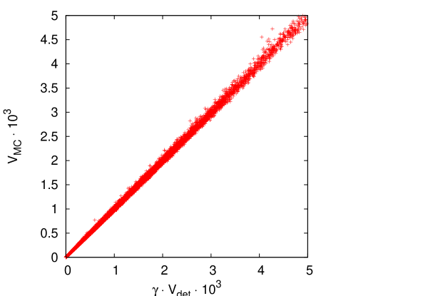
Figure 12: Cumulative distribution of $V_{MC}(T)$ and $V_{det}(T)$ (see text).

Let us note that for given accuracy of the determinant volume estimation for small tetrahedra (which is $10^{-6}$ in our case) the volume of the original tetrahedron is evaluated, in fact, with finite bias which is due to the sphericity of every small tetrahedron. However for small enough volumes the sphericity could be accounted for by simple rescaling of the determinant estimation. To calibrate the present algorithm we compared it with our previous Monte-Carlo based method. To this end we generated $5\cdot 10^{4}$ random spherical tetrahedra and applied both algorithms to each of them thus obtaining Monte-Carlo $V_{MC}(T)$ and determinant-based $V_{det}(T)$ volume estimations. Fig. 12 represents the cumulative distribution of $V_{MC}(T)$, $V_{det}(T)$, which turns out to be astonishingly narrow and is fairly compatible with linear dependence

$$V_{MC}(T)~{}=~{}\gamma\cdot V_{det}(T)\,,\qquad\gamma~{}=~{}1.1285(5)\,,$$ (A.1)

where the optimal value of $\gamma$ coefficient results from the best linear fit. Note that the plot on Fig. 12 is restricted to $V(T)\lesssim 5\cdot 10^{-3}$, which is far beyond the maximal value of topological density even for our largest spacing; however, the linear dependence (A.1) remains valid even at larger $V(T)$. Thus we are confident that the new triangulation method is definitely compatible with old Monte-Carlo approach in the relevant range of lattice spacings.

Finally, we performed the same check as one described in Boyko:2005rb . Namely, we confronted the global topological charge, which could be found unambiguously for each our configuration with one calculated with present algorithm. It turns out that they agree in all cases with no exceptions. Moreover, we found that the determinant-based algorithm gives even narrower distribution of $Q_{float}$ around integer numbers compared to that of old Monte-Carlo based approach. We conclude therefore that the new method of the topological density calculation is superior to the old one both in accuracy and performance.

References

-
(1)
I. Horvath et al.,
Phys. Rev. D 68, 114505 (2003) [arXiv:hep-lat/0302009];
Nucl. Phys. Proc. Suppl. 129, 677 (2004) [arXiv:hep-lat/0308029];
Phys. Lett. B 612, 21 (2005) [arXiv:hep-lat/0501025];
I. Horvath, Nucl. Phys. B 710, 464 (2005) [Erratum-ibid. B 714, 175 (2005)] [arXiv:hep-lat/0410046];
A. Alexandru, I. Horvath and J. b. Zhang, Phys. Rev. D 72, 034506 (2005) [arXiv:hep-lat/0506018]. -
(2)
C. Gattringer, M. Gockeler, P. E. L. Rakow, S. Schaefer and A. Schafer,
Nucl. Phys. B 617, 101 (2001) [arXiv:hep-lat/0107016];
C. Aubin et al. [MILC Collaboration], Nucl. Phys. Proc. Suppl. 140, 626 (2005) [arXiv:hep-lat/0410024];
C. Bernard et al., PoS LAT2005, 299 (2005) [arXiv:hep-lat/0510025]. -
(3)
Y. Koma, E. M. Ilgenfritz, K. Koller, G. Schierholz, T. Streuer and V. Weinberg,
PoS LAT2005, 300 (2005) [arXiv:hep-lat/0509164];
E. M. Ilgenfritz, K. Koller, Y. Koma, G. Schierholz, T. Streuer and V. Weinberg, arXiv:hep-lat/0512005. - (4) I. Horvath et al., Phys. Lett. B 617, 49 (2005) [arXiv:hep-lat/0504005].
- (5) F. V. Gubarev, S. M. Morozov, M. I. Polikarpov and V. I. Zakharov, JETP Letters 82, 381 (2005) [arXiv:hep-lat/0505016]; PoS LAT2005, 143 (2005) [arXiv:hep-lat/0510098].
- (6) V. I. Zakharov, ’Matter of resolution: From quasiclassics to fine tuning’, arXiv:hep-ph/0602141.
-
(7)
M. I. Polikarpov, S. N. Syritsyn and V. I. Zakharov,
JETP Lett. 81, 143 (2005) [Pisma Zh. Eksp. Teor. Fiz. 81, 177 (2005)] [arXiv:hep-lat/0402018];
A. V. Kovalenko, M. I. Polikarpov, S. N. Syritsyn and V. I. Zakharov, Phys. Lett. B 613, 52 (2005) [arXiv:hep-lat/0408014]; PoS LAT2005, 328 (2005) [arXiv:hep-lat/0510020]. -
(8)
V. G. Bornyakov, M. N. Chernodub, F. V. Gubarev, M. I. Polikarpov, T. Suzuki, A. I. Veselov and V. I. Zakharov,
Phys. Lett. B 537, 291 (2002) [arXiv:hep-lat/0103032];
M. N. Chernodub and V. I. Zakharov, Nucl. Phys. B 669, 233 (2003) [arXiv:hep-th/0211267];
V. G. Bornyakov, P. Y. Boyko, M. I. Polikarpov and V. I. Zakharov, Nucl. Phys. B 672, 222 (2003) [arXiv:hep-lat/0305021];
V. I. Zakharov, Nucl. Phys. Proc. Suppl. 121, 325 (2003); arXiv:hep-ph/0312210;
V. G. Bornyakov, P. Y. Boyko, M. I. Polikarpov and V. I. Zakharov, Nucl. Phys. Proc. Suppl. 129, 668 (2004) [arXiv:hep-lat/0309021];
A. V. Kovalenko, M. I. Polikarpov, S. N. Syritsyn and V. I. Zakharov, Phys. Rev. D 71, 054511 (2005) [arXiv:hep-lat/0402017]. -
(9)
F. V. Gubarev, A. V. Kovalenko, M. I. Polikarpov, S. N. Syritsyn and V. I. Zakharov,
Phys. Lett. B 574, 136 (2003) [arXiv:hep-lat/0212003];
V. I. Zakharov, arXiv:hep-ph/0306261; arXiv:hep-ph/0306262; arXiv:hep-ph/0309178;
V. I. Zakharov, Phys. Usp. 47, 37 (2004) [Usp. Fiz. Nauk 47, 39 (2004)];
V. I. Zakharov, arXiv:hep-ph/0309301; Phys. Atom. Nucl. 68, 573 (2005) [Yad. Fiz. 68, 603 (2005)] [arXiv:hep-ph/0410034];
V. I. Zakharov, AIP Conf. Proc. 756, 182 (2005) [arXiv:hep-ph/0501011]. - (10) F. V. Gubarev and S. M. Morozov, Phys. Rev. D 72, 076008 (2005) [arXiv:hep-lat/0509011].
- (11) P. Y. Boyko, F. V. Gubarev and S. M. Morozov, Phys. Rev. D 73, 014512 (2006) [arXiv:hep-lat/0511050].
- (12) E. M. Ilgenfritz, Y. Koma, G. Schierholz, T. Streuer and V. Weinberg, talk given at the ’Workshop on Computational Hadron Physics’, Nicosia, Cyprus, September 14-17, 2005 (unpublished).
- (13) P. E. L. Rakow, PoS LAT2005, 284 (2005) [arXiv:hep-lat/0510046].
-
(14)
E. Seiler,
Phys. Lett. B 525, 355 (2002) [arXiv:hep-th/0111125];
M. Aguado and E. Seiler, Phys. Rev. D 72, 094502 (2005) [arXiv:hep-lat/0503015]. - (15) A. V. Kovalenko, S. M. Morozov, M. I. Polikarpov and V. I. Zakharov, arXiv:hep-lat/0512036.
-
(16)
J. Fingberg, U. M. Heller and F. Karsch, Nucl. Phys. B 392, 493 (1993);
G. S. Bali, K. Schilling and A. Wachter, Phys. Rev. D 55, 5309 (1997);
G. S. Bali, K. Schilling and C. Schlichter, Phys. Rev. D 51, 5165 (1995);
B. Lucini and M. Teper, JHEP 0106, 050 (2001). - (17) C. Itzykson, J. -M. Drouffe, “Statistical Field Theory”, Cambridge Univ. Press, 1989.