Strange quarks in quenched twisted mass lattice QCD

Abstract

Two twisted doublets, one containing the up and down quarks and the other containing the strange quark with an SU(2)-flavor partner, are used for studies in the meson sector. The relevant chiral perturbation theory is presented, and quenched QCD simulations (where the partner of the strange quark is not active) are performed. Pseudoscalar meson masses and decay constants are computed; the vector and scalar mesons are also discussed. A comparison is made to the case of an untwisted strange quark, and some effects due to quenching, discretization, and the definition of maximal twist are explored.

I Introduction

Twisted mass lattice QCD (tmLQCD) is a variation on the Wilson action — essentially a chiral rotation of quark flavor doublets, acting on quark mass terms relative to Wilson terms in the action — which produces two desirable features: the removal of unphysical zero modes in quark propagatorsFetal01 and the elimination of $O(a)$ artifacts (where $a$ denotes lattice spacing) at maximal twistFR03 . A number of numerical simulations have been performed for both quenched and dynamical tmLQCD (for a recent review, see Ref. Shindler ). As well, the chiral perturbation theory for tmLQCD (tm$\chi$PT) has been developed. It differs from continuum $\chi$PT by discretization effects and is required for the extrapolation of tmLQCD data. The effective theory has also played a vital role in understanding various aspects of tmLQCD such as $O(a)$ improvement, the phase diagram, and the relationships between various definitions of maximal twistMunsterSchmidt ; Munster ; Scorzato ; SW04 ; AokiBar2004 ; SW05 ; Sharpe ; AokiBar2005 .

With an interest in the phenomenology of hadrons built of $u$, $d$ and $s$ quarks, our goal in this paper is to explore the usefulness of tmLQCD and tm$\chi$PT as applied to strange hadrons. There is no unique way to introduce the $s$ quark into the calculation. The method used here, to consider a pair of quark doublets $(u,d)$ and $(``c",s)$, is similar to the proposal of Pena et al.Pena . For the quenched simulations considered here the partner of the $s$ quark does not play an active role and should not be thought of as the physical charm quark. In this work no mass splitting is introduced within either doublet. The construction of the corresponding tm$\chi$PT formalism is a straightforward generalization of the published one-doublet formalismSW04 ; SW05 .

As noted above, applying a relative chiral twist has some valuable consequences but there are also some less desirable features that have to be dealt with. The tmLQCD action violates parity conservation so, in general, correlation functions contain contributions from states of both parities. Parity mixing can complicate, in particular, the extraction of matrix elements but this can be ameliorated by appropriate tuning of the twist angles. The tmLQCD action also breaks the flavor symmetry. For the version of tmLQCD used in this work the members of the quark doublets are degenerate in mass but are distinguished by having opposite chiral twists. This can lead to mass splittings within hadron isospin multiplets. It will be seen that charged and neutral kaons can acquire a mass-squared splitting which is roughly proportional to $a^{2}$.

To optimize the elimination of $O(a)$ lattice discretization errors one has to tune the chiral twist anglesFR03 . There is not a unique way to achieve maximal twist as has been discussed from the point of view of both effective theorySW04 ; SW05 ; Sharpe ; AokiBar2004 and simulationFarchioni04 ; ALW ; Jansen1 . A standard method for defining maximal twist uses a tuning procedure which involves the correlators of the first two isospin components of vector and axial operators with the pseudoscalar densityFar05 ; Farchioni04 ; SW05 . Using two variations of this method, we examine the mixing between the third isospin components of scalar and pseudoscalar correlators. Ideally one would like to have a tuning to maximal twist which would banish the physical pseudoscalar meson from appearing in the wrong parity correlator; the scalar meson with its quenched $\eta^{\prime}\pi^{0}$ contribution would similarly be banished from the other parity correlator. This is seen not to happen in our simulations. The mixings observed in actual simulations represent higher order discretization effects which differentiate between vector-axial tuning and scalar-pseudoscalar tuning.

In this work, we mainly use maximal twist in the doublet containing the strange quark as well as in the $(u,d)$ doublet. An alternative procedure would be to set the twist angle for the strange quark to zero or equivalently for the quenched theory to consider a twisted $(u,d)$ doublet and a flavor-singlet Wilson strange quark. The latter approach may be a viable one for doing full dynamical simulations. The twisted and untwisted strange quark actions lead to different patterns of parity mixing and flavour symmetry breaking at non-vanishing lattice spacing. We present some results obtained with an untwisted strange quark action to illustrate some of these differences.

At this point it is worth noting that there exist even other approaches for dealing with the strange quark. The proposal of Frezzotti and Rossi in Ref. FRnondegen allows for a nondegenerate doublet in a way which is suitable for dynamical simulationsFarchioni05 . In the limit where quark masses are degenerate within each doublet, it is equivalent to the scheme used in this paper. However, for nondegenerate quarks, twist and quark-mass splitting are associated with different flavor transformation generators. The fermion action contains terms which mix flavors so that flavor symmetry breaking effects would be more complicated to deal with in simulations and in the effective theory than for the tmLQCD action considered in this work. A further example is Ref. dimop where options for tmLQCD chosen to facilitate the calculation of the so-called kaon bag parameter are discussed.

In addition to meson masses, the pseudoscalar meson decay constants are also considered. With quark masses fixed by physical meson masses, the decay constants $f_{\pi}$ and $f_{K}$ become absolute predictions, and are shown to compare favorably with previous quenched simulations using other actions. All results are consistent with tm$\chi$PT.

The remainder of the article is organized as follows. Section II defines the effective chiral Lagrangian with two twisted flavor doublets, and Sec. III uses that Lagrangian to derive expressions involving the pseudoscalar masses and decay constants. Section IV presents the tmLQCD action and explains the parameter choices for our numerical simulations, then Sec. V discusses results obtained for the pseudoscalar and vector mesons. Scalar-pseudoscalar mixing is studied in Sec. VI, and a direct comparison to kaons built from untwisted strange quarks is given in Sec. VII. Section VIII contains the conclusions of our work. Details of currents and densities in tm$\chi$PT are collected in the Appendix.

II The effective chiral Lagrangian

To build four-flavor tm$\chi$PT, we begin from tmLQCD with two quark doublets,

$$\psi_{l}=\begin{pmatrix}u\\ d\end{pmatrix}\,,\qquad\psi_{h}=\begin{pmatrix}c\\ s\end{pmatrix}\,,$$ (1)

referred to as the light and heavy doublets respectively. Note that the choice of flavor labels is a convention; in Ref. Pena for example, a different choice is made. In this work each doublet is taken to be degenerate, so the $c$ quark, which is not active in any of our quenched tmLQCD simulations, should not be viewed as the physical charm quark. Pena et al.Pena discuss the extension of this case to the case of a nondegenerate doublet where the quark-mass splitting is aligned with the twist, preserving the favorable feature of no flavor mixing. The fermion determinant does not remain real under this generalization so this would not lead a suitable action for nonquenched simulations. However, this action may still be useful for valence quarks in a mixed action scenario as discussed, for example, in the context of tmLQCD in Ref. mixedaction .

In the so-called “twisted basis”Fetal01 ; FR03 , the two-doublet lattice action is simply a block-diagonal version of two copies of the one-doublet theory (the form of which can be found in Refs. Fetal01 ; FR03 ):

$$S^{L}_{F} =a^{4}\sum_{x}\bar{\Psi}(x)\Big{[}\frac{1}{2}\sum_{\mu}\gamma_{\mu}(\nabla^{\star}_{\mu}+\nabla_{\mu})-\frac{a}{2}\sum_{\mu}\nabla^{\star}_{\mu}\nabla_{\mu}+\boldsymbol{m_{0}}+i\gamma_{5}\boldsymbol{\mu_{0}}\Big{]}\Psi(x)\,,$$ (2)

where $\nabla_{\mu}$ and $\nabla^{\star}_{\mu}$ are the usual covariant forward and backward lattice derivatives respectively, and

$$\Psi=\begin{pmatrix}\psi_{l}\\ \psi_{h}\end{pmatrix}\,,\qquad\boldsymbol{m_{0}}=\begin{pmatrix}m_{l,\,0}\mathbb{1}_{2}&0\\ 0&m_{h,\,0}\mathbb{1}_{2}\end{pmatrix}\,,\qquad\boldsymbol{\mu_{0}}=\begin{pmatrix}\mu_{l,\,0}\tau_{3}&0\\ 0&\mu_{h,\,0}\tau_{3}\end{pmatrix}\,,$$ (3)

with $\mathbb{1}_{n}$ the $n$-by-$n$ identity matrix. The matrix $\tau_{3}$ acts in (two-)flavor space and is normalized so that $\tau_{3}^{2}=\mathbb{1}_{2}$. The parameters $m_{p,\,0}$ and $\mu_{p,\,0}$ are the normal bare and twisted masses respectively, with $p=l,\,h$.

Applying the now familiar two-step procedure of Ref. SS98 , an effective chiral Lagrangian describing the low energy physics of tmLQCD with two degenerate quark doublets can be built as a straightforward generalization of the one-doublet case detailed in Refs. RupakShoresh ; BarRupakShoresh1 ; SW04 ; SW05 . From a similar analysis described in Ref. SW04 , the form of the effective continuum Lagrangian at the quark level is found to be identical to that in the one-doublet case:

$$\mathcal{L}_{\rm eff} =\mathcal{L}_{g}+\bar{\Psi}(D\!\!\!\!/+\boldsymbol{m}+i\gamma_{5}\,\boldsymbol{\mu})\Psi+b_{SW}\,a\,\bar{\Psi}i\sigma_{\mu\nu}F_{\mu\nu}\Psi+O(a^{2})\,,$$ (4)

where $\mathcal{L}_{g}$ is the continuum gluon Lagrangian, and the physical normal and twisted mass parameters, $\boldsymbol{m}$ and $\boldsymbol{\mu}$, are defined analogously as in the one-doublet case:

$$\boldsymbol{m} \equiv \begin{pmatrix}m_{l}&0\\ 0&m_{h}\end{pmatrix}=\begin{pmatrix}Z_{m,\,l}(m_{l,\,0}-\widetilde{m}_{c,l})&0\\ 0&Z_{m,\,h}(m_{h,\,0}-\widetilde{m}_{c,h})\end{pmatrix}\,,$$ (5)

$$\boldsymbol{\mu} \equiv \begin{pmatrix}\mu_{l}\tau_{3}&0\\ 0&\mu_{h}\tau_{3}\end{pmatrix}=\begin{pmatrix}Z_{\mu,\,l}\mu_{l,\,0}\tau_{3}&0\\ 0&Z_{\mu,\,h}\mu_{h,\,0}\tau_{3}\end{pmatrix}=\begin{pmatrix}Z_{P,\,l}^{-1}\mu_{l,\,0}\tau_{3}&0\\ 0&Z_{P,\,h}^{-1}\mu_{h,\,0}\tau_{3}\end{pmatrix}\,,$$ (6)

with $Z_{P,\,l}$ and $Z_{P,\,h}$ being the matching factors for the pseudoscalar density. The quantities $\widetilde{m}_{c,\,l}$ and $\widetilde{m}_{c,\,h}$ are the critical masses, aside from an $O(a)$ shift (see Refs. RupakShoresh ; BarRupakShoresh1 ; SW04 ; SW05 and discussions below). Lattice symmetries forbid additive renormalization of $\mu_{l,\,0}$ and $\mu_{h,\,0}$. As an aside, we note that symmetries also cause the ultraviolet divergent parts of $\widetilde{m}_{c,\,l}$ and $\widetilde{m}_{c,\,h}$ to be identical. One can choose a definition of maximal twist (it will be called method (ii) in Sec. IV) for which $\widetilde{m}_{c,\,l}=\widetilde{m}_{c,\,h}$, but here we do not restrict the discussion to that special case.

Working to NLO in the power counting scheme,

$$m_{l}\sim m_{h}\sim\mu_{l}\sim\mu_{h}\sim p^{2}\sim a\Lambda_{QCD}^{2}\,,$$ (7)

the effective chiral Lagrangian found from matching reads

$$\mathcal{L}_{\chi} =\frac{f^{2}}{4}\mathrm{Tr}(D_{\mu}\Sigma D_{\mu}\Sigma^{\dagger})-\frac{f^{2}}{4}\mathrm{Tr}(\chi^{\dagger}\Sigma+\Sigma^{\dagger}\chi)-\frac{f^{2}}{4}\mathrm{Tr}(\hat{A}^{\dagger}\Sigma+\Sigma^{\dagger}\hat{A})$$

$$\quad-L_{1}\big{[}\mathrm{Tr}(D_{\mu}\Sigma D_{\mu}\Sigma^{\dagger})\big{]}^{2}-L_{2}\mathrm{Tr}(D_{\mu}\Sigma D_{\nu}\Sigma^{\dagger})\mathrm{Tr}(D_{\mu}\Sigma D_{\nu}\Sigma^{\dagger})-L_{3}\mathrm{Tr}\big{[}(D_{\mu}\Sigma D_{\mu}\Sigma^{\dagger})^{2}\big{]}$$

$$\quad+L_{4}\mathrm{Tr}(D_{\mu}\Sigma^{\dagger}D_{\mu}\Sigma)\mathrm{Tr}(\chi^{\dagger}\Sigma+\Sigma^{\dagger}\chi)+L_{5}\mathrm{Tr}\left[(D_{\mu}\Sigma D_{\mu}\Sigma^{\dagger})(\chi\Sigma^{\dagger}+\Sigma\chi^{\dagger})\right]$$

$$\quad-L_{6}\big{[}\mathrm{Tr}(\chi^{\dagger}\Sigma+\Sigma^{\dagger}\chi)\big{]}^{2}-L_{7}\big{[}\mathrm{Tr}(\chi^{\dagger}\Sigma-\Sigma^{\dagger}\chi)\big{]}^{2}-L_{8}\mathrm{Tr}\big{[}(\chi^{\dagger}\Sigma+\Sigma^{\dagger}\chi)^{2}\big{]}$$

$$\quad+iL_{9}\mathrm{Tr}(L_{\mu\nu}D_{\mu}\Sigma D_{\nu}\Sigma^{\dagger}+R_{\mu\nu}D_{\mu}\Sigma^{\dagger}D_{\nu}\Sigma)+L_{10}\mathrm{Tr}(L_{\mu\nu}\Sigma R_{\mu\nu}\Sigma^{\dagger})$$

$$\quad+W_{4}\mathrm{Tr}(D_{\mu}\Sigma^{\dagger}D_{\mu}\Sigma)\mathrm{Tr}(\hat{A}^{\dagger}\Sigma+\Sigma^{\dagger}\hat{A})+W_{5}\mathrm{Tr}\big{[}(D_{\mu}\Sigma D_{\mu}\Sigma^{\dagger})(\hat{A}\Sigma^{\dagger}+\Sigma\hat{A}^{\dagger})\big{]}$$

$$\quad-W_{6}\mathrm{Tr}(\chi^{\dagger}\Sigma+\Sigma^{\dagger}\chi)\mathrm{Tr}(\hat{A}^{\dagger}\Sigma+\Sigma^{\dagger}\hat{A})-W_{6}^{\prime}\big{[}\mathrm{Tr}(\hat{A}^{\dagger}\Sigma+\Sigma^{\dagger}\hat{A})\big{]}^{2}$$

$$\quad-W_{7}\mathrm{Tr}(\chi^{\dagger}\Sigma-\Sigma^{\dagger}\chi)\mathrm{Tr}(\hat{A}^{\dagger}\Sigma-\Sigma^{\dagger}\hat{A})-W_{7}^{\prime}\big{[}\mathrm{Tr}(\hat{A}^{\dagger}\Sigma-\Sigma^{\dagger}\hat{A})\big{]}^{2}$$

$$\quad-W_{8}\mathrm{Tr}\big{[}(\chi^{\dagger}\Sigma+\Sigma^{\dagger}\chi)(\hat{A}^{\dagger}\Sigma+\Sigma^{\dagger}\hat{A})\big{]}-W_{8}^{\prime}\mathrm{Tr}\big{[}(\hat{A}^{\dagger}\Sigma+\Sigma^{\dagger}\hat{A})^{2}\big{]}$$

$$\quad+W_{10}\mathrm{Tr}(D_{\mu}\hat{A}^{\dagger}D_{\mu}\Sigma+D_{\mu}\Sigma^{\dagger}D_{\mu}\hat{A})$$

$$\quad+H_{1}\mathrm{Tr}(L_{\mu\nu}L_{\mu\nu}+R_{\mu\nu}R_{\mu\nu})-H_{2}\mathrm{Tr}(\chi^{\dagger}\chi)-H_{2}^{\prime}\mathrm{Tr}(\hat{A}^{\dagger}\chi+\chi^{\dagger}\hat{A})-H_{3}\mathrm{Tr}(\hat{A}^{\dagger}\hat{A})\,,$$ (8)

where the $\Sigma$ field is now $SU(4)$ matrix-valued, and transforms under the chiral group $SU(4)_{L}\times SU(4)_{R}$. Note that $\mathcal{L}_{\chi}$ has basically the same form as that in the $SU(2)$ theoryRupakShoresh ; BarRupakShoresh1 ; SW04 ; SW05 , except that terms linearly dependent under $SU(2)$ are no longer so under $SU(4)$.

The quantities $\chi$ and $\hat{A}$ are spurions for the quark masses and discretization errors, respectivelyBarRupakShoresh2 . At the end of the analysis they are set to the constant values

$$\chi\longrightarrow 2B_{0}(\boldsymbol{m}+i\boldsymbol{\mu})\,,\qquad\qquad\hat{A}\longrightarrow 2W_{0}\,a\,\mathbb{1}_{4}\,,$$ (9)

where $B_{0}$ and $W_{0}$ are unspecified constants having dimensions [mass] and [mass³] respectively. Notice that $\hat{A}$ involves a single flavour-independent Pauli term for both doublets.

The discretization effect due to the Pauli term, i.e. the term containing $b_{SW}$ in Eq. (4), can be included non-perturbatively as in Ref. SW05 by using the shifted spurion $\chi^{\prime}\equiv\chi+\hat{A}$, which corresponds at the quark level to a redefinition of the normal quark mass from $m$ to

$$m^{\prime}_{p}\equiv m_{p}+aW_{0}/B_{0}\,\qquad p=l,\,h\,.$$ (10)

This shift in turn corresponds to an $O(a)$ correction to the critical mass, so that it becomes

$$m_{c,p}=Z_{m,\,p}\widetilde{m}_{c,p}-aW_{0}/B_{0}\,\qquad p=l,\,h\,.$$ (11)

In terms of $\chi^{\prime}$, the chiral Lagrangian, Eq. (4), can be written as:

$$\mathcal{L}_{\chi} =\frac{f^{2}}{4}\mathrm{Tr}(D_{\mu}\Sigma D_{\mu}\Sigma^{\dagger})-\frac{f^{2}}{4}\mathrm{Tr}(\chi^{\prime\dagger}\Sigma+\Sigma^{\dagger}\chi^{\prime})$$

$$\quad-L_{1}\big{[}\mathrm{Tr}(D_{\mu}\Sigma D_{\mu}\Sigma^{\dagger})\big{]}^{2}-L_{2}\mathrm{Tr}(D_{\mu}\Sigma D_{\nu}\Sigma^{\dagger})\mathrm{Tr}(D_{\mu}\Sigma D_{\nu}\Sigma^{\dagger})-L_{3}\mathrm{Tr}\big{[}(D_{\mu}\Sigma D_{\mu}\Sigma^{\dagger})^{2}\big{]}$$

$$\quad+L_{4}\mathrm{Tr}(D_{\mu}\Sigma^{\dagger}D_{\mu}\Sigma)\mathrm{Tr}(\chi^{\prime\dagger}\Sigma+\Sigma^{\dagger}\chi^{\prime})+L_{5}\mathrm{Tr}\left[(D_{\mu}\Sigma D_{\mu}\Sigma^{\dagger})(\chi^{\prime}\Sigma^{\dagger}+\Sigma\chi^{\prime\dagger})\right]$$

$$\quad-L_{6}\big{[}\mathrm{Tr}(\chi^{\prime\dagger}\Sigma+\Sigma^{\dagger}\chi^{\prime})\big{]}^{2}-L_{7}\big{[}\mathrm{Tr}(\chi^{\prime\dagger}\Sigma-\Sigma^{\dagger}\chi^{\prime})\big{]}^{2}-L_{8}\mathrm{Tr}\big{[}(\chi^{\prime\dagger}\Sigma+\Sigma^{\dagger}\chi^{\prime})^{2}\big{]}$$

$$\quad+iL_{9}\mathrm{Tr}(L_{\mu\nu}D_{\mu}\Sigma D_{\nu}\Sigma^{\dagger}+R_{\mu\nu}D_{\mu}\Sigma^{\dagger}D_{\nu}\Sigma)$$

$$\quad+\widetilde{W}_{4}\mathrm{Tr}(D_{\mu}\Sigma^{\dagger}D_{\mu}\Sigma)\mathrm{Tr}(\hat{A}^{\dagger}\Sigma+\Sigma^{\dagger}\hat{A})+\widetilde{W}_{5}\mathrm{Tr}\big{[}(D_{\mu}\Sigma D_{\mu}\Sigma^{\dagger})(\hat{A}\Sigma^{\dagger}+\Sigma\hat{A}^{\dagger})\big{]}$$

$$\quad-\widetilde{W}_{6}\mathrm{Tr}(\chi^{\prime\dagger}\Sigma+\Sigma^{\dagger}\chi^{\prime})\mathrm{Tr}(\hat{A}^{\dagger}\Sigma+\Sigma^{\dagger}\hat{A})-\widetilde{W}_{6}^{\prime}\big{[}\mathrm{Tr}(\hat{A}^{\dagger}\Sigma+\Sigma^{\dagger}\hat{A})\big{]}^{2}$$

$$\quad-\widetilde{W}_{7}\mathrm{Tr}(\chi^{\prime\dagger}\Sigma-\Sigma^{\dagger}\chi^{\prime})\mathrm{Tr}(\hat{A}^{\dagger}\Sigma-\Sigma^{\dagger}\hat{A})-\widetilde{W}_{7}^{\prime}\big{[}\mathrm{Tr}(\hat{A}^{\dagger}\Sigma-\Sigma^{\dagger}\hat{A})\big{]}^{2}$$

$$\quad-\widetilde{W}_{8}\mathrm{Tr}\big{[}(\chi^{\prime\dagger}\Sigma+\Sigma^{\dagger}\chi^{\prime})(\hat{A}^{\dagger}\Sigma+\Sigma^{\dagger}\hat{A})\big{]}-\widetilde{W}_{8}^{\prime}\mathrm{Tr}\big{[}(\hat{A}^{\dagger}\Sigma+\Sigma^{\dagger}\hat{A})^{2}\big{]}$$

$$\quad+W_{10}\mathrm{Tr}(D_{\mu}\hat{A}^{\dagger}D_{\mu}\Sigma+D_{\mu}\Sigma^{\dagger}D_{\mu}\hat{A})$$

$$\quad-H_{2}\mathrm{Tr}(\chi^{\prime\dagger}\chi^{\prime})-\widetilde{H}_{2}^{\prime}\mathrm{Tr}(\hat{A}^{\dagger}\chi^{\prime}+\chi^{\prime\dagger}\hat{A})\,,$$ (12)

where terms that lead only to contact terms in correlation functions and are hence not needed below, viz. the $L_{10}$, $H_{1}$ and $H_{3}$ terms, have been dropped. We have also introduced useful combinations

$$\widetilde{W}_{i} =W_{i}-L_{i}\,,\quad i=4,\,5$$

$$\widetilde{W}_{j} =W_{j}-2L_{j}\,,\quad\widetilde{W}_{j}^{\prime}=W_{j}^{\prime}-W_{j}+2L_{j}\,,\quad j=6,\,7,\,8$$

$$\widetilde{H}_{2}^{\prime} =H_{2}^{\prime}-H_{2}\,.$$ (13)

As noted in Ref. SW05 , the $W_{10}$ term is redundant. It can be transformed away by the change of variables

$$\delta\Sigma=\frac{2W_{10}}{f^{2}}(\Sigma\hat{A}^{\dagger}\Sigma-\hat{A})\,.$$ (14)

This transforms the $W_{10}$ term into the $\widetilde{W}_{5}$, $\widetilde{W}_{8}$, and $\widetilde{H}_{2}^{\prime}$ terms with their coefficients shifted to $\widetilde{W}_{5}+W_{10}$, $\widetilde{W}_{8}+W_{10}/2$, and $\widetilde{H}_{2}^{\prime}-W_{10}$, respectively. All physical quantities must depend then only on these combinations and not on $W_{10}$, $\widetilde{W}_{5}$, $\widetilde{W}_{8}$, and $\widetilde{H}_{2}^{\prime}$ separately. We have kept the $W_{10}$ term because it provides a useful diagnostic in tm$\chi$PT calculations.

III Chiral perturbation theory for generic small masses

In this section, we work out the consequences of the $SU(4)$ effective chiral Lagrangian, Eq. (II), which generalizes the results of the $SU(2)$ theory of Ref. SW05 , and our focus will be on the masses and decay constants of kaons: pseudoscalar mesons that involve both flavor doublets. We work in the “generic small mass” regime defined by

$$\Lambda_{\chi}^{2}\gg M_{h}^{\prime}\gtrsim M_{l}^{\prime}\gtrsim 2W_{0}\,a\,,$$ (15)

where $\Lambda_{\chi}=4\pi f$ and

$$M_{p}^{\prime}=2B_{0}\sqrt{m_{p}^{{}^{\prime}2}+\mu_{p}^{2}}\,,\qquad p=l,\,h\,.$$ (16)

Note that $M_{p}^{\prime}$ has dimension [mass²]. In the analysis of our numerical data, quenching effects will also be considered (see Eqs. (43)–(45)).

III.1 The vacuum

At LO the discretized Lagrangian retains its continuum form, so the LO vacuum expectation value (VEV) of $\Sigma$ is that which cancels out the twists in the shifted mass matrix:

$$\langle 0|\Sigma|0\rangle_{LO}\equiv\Sigma_{0}\equiv\begin{pmatrix}\exp(i\omega_{l,\,0}\tau_{3})&0\\ 0&\exp(i\omega_{h,\,0}\tau_{3})\end{pmatrix}\,,$$ (17)

where $\omega_{p,\,0}$ are defined by

$$c_{p,\,0}\equiv\cos(\omega_{p,\,0})=2B_{0}m^{\prime}/M_{p}^{\prime}\,,\qquad s_{p,\,0}\equiv\sin(\omega_{p,\,0})=2B_{0}\mu_{p}/M_{p}^{\prime}\,,\qquad p=l,\,h\,.$$ (18)

This provides one definition for the twist angles.

At NLO, the VEV of $\Sigma$ is realigned by a small amount from $\Sigma_{0}$. Defining

$$\langle 0|\Sigma|0\rangle_{NLO}\equiv\Sigma_{m}\equiv\begin{pmatrix}\exp(i\omega_{l,\,m}\tau_{3})&0\\ 0&\exp(i\omega_{h,\,m}\tau_{3})\end{pmatrix}\,,\quad\omega_{p,\,m}=\omega_{p,\,0}+\epsilon_{p}\,,\quad p=l,\,h\,,$$ (19)

the shifts from LO, $\epsilon_{l,\,h}$, are found from minimizing the potential to be

$$\epsilon_{p}=-\frac{16W_{0}as_{p,\,0}}{f^{2}}\left\{2\widetilde{W}_{6}\,(M_{l}^{\prime}+M_{h}^{\prime})/M_{p}^{\prime}+\widetilde{W}_{8}+\frac{4W_{0}a}{M_{p}^{\prime}}\big{[}\widetilde{W}_{6}^{\prime}\,(c_{l,\,0}+c_{h,\,0})+\widetilde{W}_{8}^{\prime}\,c_{p,\,0}\big{]}\right\}\,.$$ (20)

Expanding about the VEV as in Ref. SW05 , the physical pion fields are defined by

$$\Sigma=\xi_{m}\Sigma_{ph}\xi_{m}\,,\quad\xi_{m}=\begin{pmatrix}\exp(i\omega_{l,\,m}\tau_{3}/2)&0\\ 0&\exp(i\omega_{h,\,m}\tau_{3}/2)\end{pmatrix}\,,\quad\Sigma_{ph}=\exp(i\Phi/f)\,,$$ (21)

where $\Phi$ has the representation

$$\frac{1}{\sqrt{2}}\,\Phi \equiv\frac{1}{\sqrt{2}}\sum_{i=1}^{15}\varphi_{i}\,\Lambda_{i}$$

$$=\begin{pmatrix}\frac{1}{\sqrt{2}}\,\pi^{0}+\frac{1}{\sqrt{6}}\,\eta_{8}+\frac{1}{\sqrt{12}}\,\eta_{15}&\pi^{+}&\overline{D}^{0}&K^{+}\\ \pi^{-}&-\frac{1}{\sqrt{2}}\,\pi^{0}+\frac{1}{\sqrt{6}}\,\eta_{8}+\frac{1}{\sqrt{12}}\,\eta_{15}&D^{-}&K^{0}\\ D^{0}&D^{+}&-\frac{3}{\sqrt{12}}\,\eta_{15}&D^{+}_{s}\\ K^{-}&\overline{K}^{0}&D^{-}_{s}&-\frac{2}{\sqrt{6}}\,\eta_{8}+\frac{1}{\sqrt{12}}\,\eta_{15}\end{pmatrix}\,.$$ (22)

Our choice of the fifteen generators of $SU(4)$, $\Lambda_{1},\ldots,\Lambda_{15}$, differ slightly from the conventional ones. Here, all off-diagonal generators and the diagonal $\Lambda_{3}$ are the same as the conventional ones, but we choose the rest of the diagonal generators to be such that the $(3,3)$ and $(4,4)$ entries of the diagonal $\Lambda_{8}$ and $\Lambda_{15}$ are interchanged with respect to the conventional ones. This maintains consistency with the ordering of quark fields ($u$, $d$, $c$, $s$), used throughout this work, and allows for the standard meson naming convention. In particular, we have for the flavor-diagonal components of $\Phi$:

$$|\pi^{0}\rangle = \frac{1}{\sqrt{2}}\bigg{(}|u\bar{u}\rangle-|d\bar{d}\rangle\bigg{)}\,,$$ (23)

$$|\eta_{8}\rangle = \frac{1}{\sqrt{6}}\bigg{(}|u\bar{u}\rangle+|d\bar{d}\rangle-2|s\bar{s}\rangle\bigg{)}\,,$$ (24)

$$|\eta_{15}\rangle = \frac{1}{\sqrt{12}}\bigg{(}|u\bar{u}\rangle+|d\bar{d}\rangle+|s\bar{s}\rangle-3|c\bar{c}\rangle\bigg{)}\,.$$ (25)

Note that the $c$ quark is mass-degenerate with the $s$ quark, so pairs of $D$’s and $K$’s related by the interchange of $c$ and $s$ quarks are mass-degenerate at LO in the chiral expansion. By inserting the above expansion of $\Sigma$ into the chiral Lagrangian, Eq. (II), the Feynman rules for the $SU(4)$ theory can be straightforwardly obtained.

III.2 Defining the twist angle

In the continuum, the twist angle for each degenerate doublet can be defined unambiguously by

$$\omega_{p}=\tan^{-1}(\mu_{p}/m_{p})\,,\qquad p=l,\,h\,.$$ (26)

Given the twist angles, the off-diagonal $SU(4)$ components of physical currents and densities are related to their counterparts in the twisted basis by (with a “hat” denoting the physical basis)

$$\hat{V}^{a}_{\mu} =\cos(\Delta^{a}\omega)V^{a}_{\mu}+\eta_{ab}\sin(\Delta^{a}\omega)A^{b}_{\mu}\,,$$

$$\hat{A}^{a}_{\mu} =\cos(\Delta^{a}\omega)A^{a}_{\mu}+\eta_{ab}\sin(\Delta^{a}\omega)V^{b}_{\mu}\,,$$

$$\hat{S}^{a} =\cos(\Sigma^{a}\omega)S^{a}+i\sin(\Sigma^{a}\omega)P^{a}\,,$$

$$\hat{P}^{a} =\cos(\Sigma^{a}\omega)P^{a}+i\sin(\Sigma^{a}\omega)S^{a}\,,$$

$$a,\,b \in\mathfrak{K}\backslash\mathfrak{D}\,,\qquad\mathfrak{K}=\{1,\ldots,15\}\,,\qquad\mathfrak{D}=\{3,\,8,\,15\}\,,$$ (27)

where

$$\eta_{ab}=\left\{\begin{array}[]{rl}\pm 1,&{\rm for~{}}b=a\pm 1\\ 0,&{\rm otherwise}\end{array}\right.$$ (28)

and

$$\Delta^{a}\omega=\frac{1}{2}(\omega_{i_{a}}-\omega_{j_{a}})\,,\qquad\Sigma^{a}\omega=\frac{1}{2}(\omega_{i_{a}}+\omega_{j_{a}})\,,\qquad i_{a}<j_{a}\,.$$ (29)

The indices $i_{a}$ and $j_{a}$ are the row numbers of the non-zero entries of the $SU(4)$ generator $\Lambda_{a}$ that defines the particular flavor current or density, and

$$\omega_{1}=-\omega_{2}=\omega_{l}\,,\qquad\omega_{3}=-\omega_{4}=\omega_{h}\,.$$ (30)

For a thorough discussion of currents and densities, see App. A. We note now that Eq. (III.2) has the form of the inverse transformation of the LO operator, Eq. (A), except that here the twist angles are $\omega_{p}$ not $\omega_{p,\,m}$.

On a lattice, discretization errors mean that different definitions for the twist angles will lead to observables that differ by $O(a)$. In this work, we will define $\omega_{p}$ non-perturbatively as in Refs. Far05 ; Farchioni04 ; SW04 ; ALW by enforcing the absence of parity breaking in the physical basis. In particular, we will enforce

$$\langle\hat{V}^{b}_{\mu}(x)\hat{P}^{a}(y)\rangle=0\,,\qquad a,\,b\in\mathfrak{K}\backslash\mathfrak{D}\,.$$ (31)

From the definitions in Eq. (III.2), this condition gives

$$\tan\omega_{l}\equiv\frac{\langle V^{2}_{\mu}(x)P^{1}(y)\rangle}{\langle A^{1}_{\mu}(x)P^{1}(y)\rangle}\,,\qquad\tan\omega_{h}\equiv\frac{\langle V^{14}_{\mu}(x)P^{13}(y)\rangle}{\langle A^{13}_{\mu}(x)P^{13}(y)\rangle}\,.$$ (32)

The results for $\omega_{p}$ depend on the distance $|x-y|$ at $O(a)$. We will enforce the condition in Eq. (31) at long distance where the single-meson contribution dominates.

Evaluating Eq. (32) using the results in App. A, we find at LO $\omega_{p}=\omega_{p,\,m}=\omega_{p,\,0}$, since only $\hat{A}^{a}_{\mu,\,LO}$ and $P^{a}=\hat{P}^{a}$, $a\in\{1,13\}$, couple to the single-meson state. At NLO, the sole non-trivial contributions surviving in the ratios of Eq. (32) come from the $W_{10}$ term, just as in the one-doublet theory, and as in Ref. SW05 we find

$$\tan\omega_{p}=\frac{\sin\omega_{p,\,m}}{\cos\omega_{p,\,m}+\delta}\,,\qquad\delta=\frac{8W_{0}a}{f^{2}}W_{10}\,,\qquad p=l,\,h\,.$$ (33)

III.3 Kaon masses and decay constants

With the Feynman rules in hand, and the twist angles defined, we have now all that is needed to calculate pseudoscalar meson masses and matrix elements. At NLO, we find that the mass of the neutral kaon is given by

$$m^{2}_{K^{0}} = \hat{M}^{\prime}+\frac{\hat{M}^{\prime}}{6}\Big{\{}4\mathcal{I}[m_{\eta_{8}}^{2}]-\mathcal{I}[m_{\eta_{15}}^{2}]\Big{\}}$$ (34)

$$+\frac{8}{f^{2}}\Big{\{}\hat{M}^{\prime 2}\,(8L_{6}-4L_{4}+2L_{8}-L_{5})$$

$$+\hat{M}^{\prime}a\,W_{0}\,(c_{l}+c_{h})(8\widetilde{W}_{6}-4\widetilde{W}_{4}+2\widetilde{W}_{8}-\widetilde{W}_{5})$$

$$+2W_{0}^{2}\,a^{2}\,\big{[}(4\widetilde{W}_{6}^{\prime}+\widetilde{W}_{8}^{\prime})(c_{l}+c_{h})^{2}-\widetilde{W}_{8}^{\prime}\,(s_{l}+s_{h})^{2}\big{]}\Big{\}}\,,$$

where

$$\hat{M}^{\prime} = (M_{l}^{\prime}+M_{h}^{\prime})/2\,,$$ (35)

$$m_{\eta_{8}}^{2} = (M_{l}^{\prime}+2M_{h}^{\prime})/3\,,$$ (36)

$$m_{\eta_{15}}^{2} = (M_{l}^{\prime}+5M_{h}^{\prime})/6\,,$$ (37)

are respectively the LO $K$, $\eta_{8}$ and $\eta_{15}$ squared masses, and $c_{p}=\cos\omega_{p}$, $s_{p}=\sin\omega_{p}$, which we can use instead of $\cos\omega_{p,\,m}$ and $\sin\omega_{p,\,m}$ respectively at the order we work. Note that the usual continuum one-loop contributionGL85 appears in Eq. (34),

$$\mathcal{I}[m^{2}]=\frac{m^{2}}{32\pi^{2}f^{2}}\ln\frac{m^{2}}{\Lambda_{R}^{2}}\,,$$ (38)

with $\Lambda_{R}$ being the renormalization scale. Note also that, as required, the neutral kaon mass depends only on the combination $2\widetilde{W}_{8}-\widetilde{W}_{5}$ rather than on $\widetilde{W}_{8}$ and $\widetilde{W}_{5}$ separately, and that the kaon mass is automatically $O(a)$ improved at maximal twist ($c_{p}=0$).

Flavor breaking in the kaon masses at NLO is given solely by the analytic contribution, just as in the $SU(2)$ theorySW05 , and it reads

$$m^{2}_{K^{0}}-m^{2}_{K^{\pm}}=-\frac{64}{f^{2}}W_{0}^{2}\,a^{2}s_{l}s_{h}\widetilde{W}_{8}^{\prime}=-\widetilde{W}_{8}^{\prime}\,\frac{64}{f^{2}}\frac{W_{0}^{2}\,a^{2}\,\mu_{l}\,\mu_{h}}{M_{l}^{\prime}\,M_{h}^{\prime}}\,,$$ (39)

where the second equality is derived using the fact that we can replace $s_{p}$ by $s_{p,0}$ at the order we are working.

Before calculating Eq. (39) explicitly, one might have anticipated an expression that was quadruply suppressed in our power counting scheme, Eq. (7), due to the requirement of being $O(a^{2})$ and $O(\mu_{l}\mu_{h})$. However, Eq. (39) shows that the $\mu_{l}\mu_{h}$ dependence enters as a ratio with $M_{l}^{\prime}M_{h}^{\prime}$ and the squared kaon mass difference is therefore nonzero already at NLO.

With the physical axial current defined in App. A, the $K^{\pm}$ decay constant to NLO is determined to be

$$f_{K}=f\bigg{\{}1 +\frac{4}{f^{2}}\big{[}(4L_{4}+L_{5})\hat{M}^{\prime}+W_{0}\,a\,(c_{l}+c_{h})(4\widetilde{W}_{4}+\widetilde{W}_{5}+W_{10})\big{]}$$

$$-\frac{3}{4}\mathcal{I}[m_{\pi}^{2}]-\frac{3}{4}\mathcal{I}[m_{\eta_{8}}^{2}]-2\mathcal{I}[m_{K}^{2}]-\frac{1}{2}\mathcal{I}[m_{D_{s}}^{2}]\bigg{\}}\,,$$ (40)

where $m_{\pi}^{2}=M_{l}^{\prime}$, $m_{K}^{2}=m_{D}^{2}=\hat{M}^{\prime}$ and $m_{D_{s}}^{2}=M_{h}^{\prime}$ are the LO expressions for the pion, kaon and $D_{s}$ squared masses respectively. Our tm$\chi$PT conventions are such that $f_{\pi}\approx 93$ MeV. Note that the one-loop contributions from the pions and the $\eta_{8}$ are the same as in the continuum $SU(3)$ theoryGL85 . Flavor breaking effects enter first at $O(a^{2})$, which is NNLO for decay constants. The above result shows that the decay constant depends only on the combination $\widetilde{W}_{5}+W_{10}$, and is automatically $O(a)$ improved at maximal twist.

IV Simulation details

We have performed quenched simulations using the action of Eq. (2). The ensembles computed in Ref. ALW , containing 300 gauge configurations each at $\beta=5.85$ and $\beta=6.0$, have subsequently been extended to include 600 configurations eachALWdublin . An additional ensemble at $\beta=6.2$ has also been generated, again using a pseudo-heatbath algorithm which acts on all $SU(2)$ subgroups. Quark propagators are obtained from a 1-norm quasi-minimal residual algorithm, with periodic boundary conditions in all directions. Simulation parameters are collected in Table 1.

To remove $O(a)$ errors, simulations must be done at maximal twist, and to that end we employ Eq. (32) implemented, following Refs. Far05 ; Farchioni04 ; ALW by

$$\tan\omega_{l} = \frac{i\sum_{\vec{x}}\left<V_{4}^{1-i2}(\vec{x},t)P^{1+i2}(0)\right>}{\sum_{\vec{x}}\left<A_{4}^{1-i2}(\vec{x},t)P^{1+i2}(0)\right>}\,,$$ (41)

$$\tan\omega_{h} = \frac{i\sum_{\vec{x}}\left<V_{4}^{13-i14}(\vec{x},t)P^{13+i14}(0)\right>}{\sum_{\vec{x}}\left<A_{4}^{13-i14}(\vec{x},t)P^{13+i14}(0)\right>}\,.$$ (42)

where ${\cal O}^{a+ib}\equiv({\cal O}^{a}+i{\cal O}^{b})/\sqrt{2}$. This method of tuning separately at each twisted quark mass is only one possible choice. A nice summary of the situation in the generic small mass regime (Eq. (15)) that we are using has been given by Sharpe in Ref. Sharpe . In the language of that article, we are using method (i). A variant, called method (ii), extrapolates the results of method (i) to the point of vanishing twisted mass, and then uses that definition of maximal twist for all values of $\mu_{p,\,0}$ ($p=l,h$). Another option, called method (iii), relies on twistings in the scalar-pseudoscalar sector rather than the vector-axial sector. Method (iv) assumes that maximal twist can be sufficiently well defined by simply holding the hopping parameter fixed at its critical value from the untwisted Wilson theory.

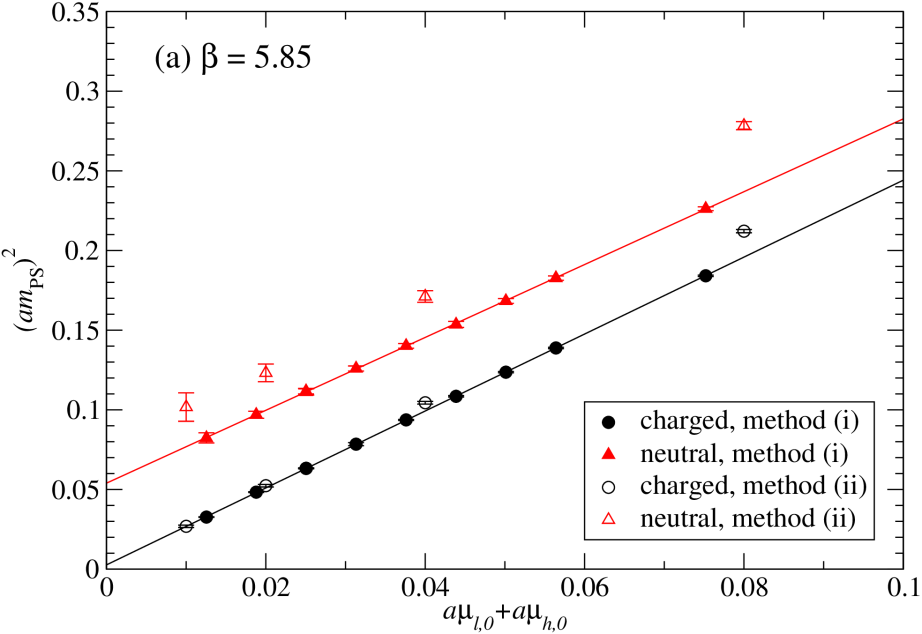
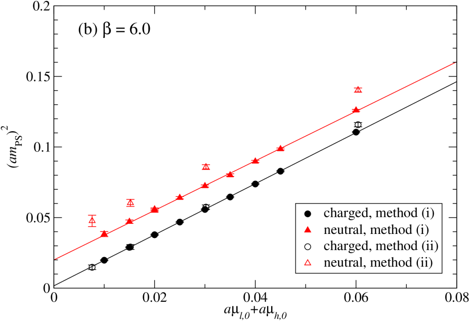
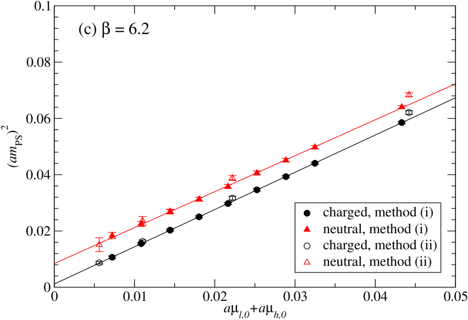
Figure 1: Pseudoscalar meson mass squared as a function of the sum of quark and antiquark twisted mass parameters. Subscripts $l$ and $h$ indicate the light and heavy doublets. Results labelled by method (i) are from the present work; results labelled by method (ii) are from Ref. flavorbreaking and have equal masses for the quark and anti-quark. Straight lines are linear fits to the data from method (i).

As sketched in Fig. 1 of Ref. Sharpe , methods (i), (ii) and (iii) are all acceptable non-perturbative definitions of maximal twist, and are superior to method (iv). Though most of our simulations use method (i), we will make frequent comparisons with results from the $\chi$LF collaborationflavorbreaking ; scaling using method (ii). We will also present our own results from method (ii) when discussing aspects of scalar correlators in Sec. VI.

Throughout this work, only local operators are used, and error bars reported in graphs and tables are statistical only. All statistical uncertainties are obtained from the bootstrap method with replacement, where the number of bootstrap ensembles is three times the number of data points in the original ensemble. Masses and decay constants are obtained from unconstrained three-state fits to correlators, using all time steps except the source. In the following sections, each discussion includes references to the relevant figures, but we note here that the corresponding numerical values are collected in Table 2.

V Pseudoscalar and vector mesons

Masses of the charged and neutral kaons, i.e. the ground state pseudoscalar mesons containing one $s$ (anti)quark from the heavy doublet and one $u$ or $d$ (anti)quark from the light doublet, are plotted in Fig. 1. Both twisted masses, $a\mu_{l,\,0}$ and $a\mu_{h,\,0}$, take on all values from Table 1 and the normal mass term is tuned accordingly (also shown in Table 1) to achieve maximal twist at each particular twisted mass value.

These data are expected to be consistent with a quenched versionquench1 ; quench2 ; CPPACS of Eq. (34), which at maximal twist reads

$$m^{2}_{K^{0}} =\hat{M}^{\prime}\left[1-\delta_{\rm quench}\left(\ln\frac{M_{l}^{\prime}}{(4\pi f)^{2}}+\frac{M_{h}^{\prime}}{M_{h}^{\prime}-M_{l}^{\prime}}\ln\frac{M_{h}^{\prime}}{M_{l}^{\prime}}\right)\right]$$

$$\quad+\frac{8\hat{M}^{\prime 2}}{f^{2}}(8L_{6}-4L_{4}+2L_{8}-L_{5})-\frac{64}{f^{2}}a^{2}W_{0}^{2}\widetilde{W}_{8}^{\prime}$$ (43)

$$=\hat{M}^{\prime}-\frac{64}{f^{2}}a^{2}W_{0}^{2}\widetilde{W}_{8}^{\prime}+O(M_{p}^{\prime 2})+O(\hat{M}^{\prime}\delta_{\rm quench})\,,\qquad p=l,h\,,$$ (44)

$$m^{2}_{K^{\pm}} =m^{2}_{K^{0}}+\frac{64}{f^{2}}a^{2}W_{0}^{2}\widetilde{W}_{8}^{\prime}$$

$$=\hat{M}^{\prime}+O(M_{p}^{\prime 2})+O(\hat{M}^{\prime}\delta_{\rm quench})\,,\qquad p=l,h\,,$$ (45)

where $\delta_{\rm quench}$ is the standard coefficient for the quenched logarithm. As Fig. 1 indicates, linear fits in $\hat{M}^{\prime}$ to the data at each $\beta$ value yield excellent results, so $O(M_{p}^{\prime 2})$ and $O(\hat{M}^{\prime}\delta_{\rm quench})$ effects are largely unnecessary. Notice in particular that our linear fit for the charged kaon did lead to a nonzero (but small) residual kaon mass at $\hat{M}^{\prime}=0$, thus reminding us that corrections to the linear form are important for such details. We have verified, for example, that the function $A\hat{M}^{\prime}+B\hat{M}^{\prime}\ln\hat{M}^{\prime}$ yields an equally excellent fit to our data, and of course it enforces the absence of any residual mass at $\hat{M}^{\prime}=0$.

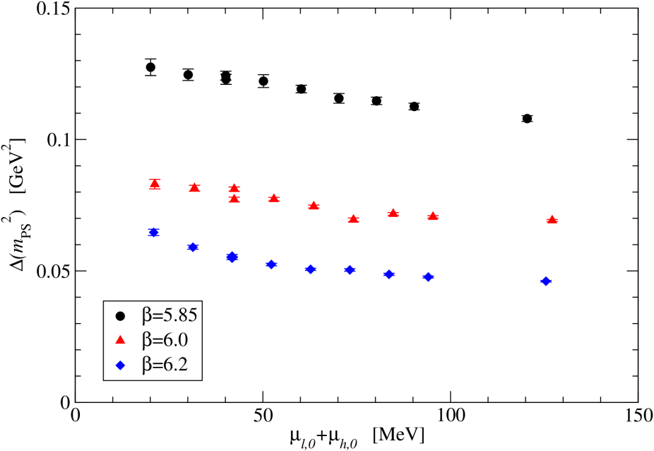
Figure 2: The difference between charged and neutral squared pseudoscalar meson masses as a function of the sum of quark and antiquark twisted masses. Subscripts $l$ and $h$ indicate the light and heavy doublets.

Fig. 1 also reveals differences between our results with method (i) and results from the $\chi$LF collaborationflavorbreaking using equal quark and antiquark masses with method (ii). For charged mesons, the method (i) mass difference is smaller than the method (ii) difference, and as expected from tm$\chi$PT the chiral limits appear to be very similar. For neutral mesons, the chiral limits appear to be somewhat different on the coarser lattices, particularly at $\beta=6.0$, but become consistent at $\beta=6.2$. We recall from Fig. 2 of Ref. flavorbreaking that the $\chi$LF data at $\beta=6.0$ happen to be statistically above their fitted $a^{2}$ extrapolation, so we see no essential disagreement among any of the data sets displayed in our Fig. 1.

The difference between the squared masses of charged and neutral kaons is plotted directly in Fig. 2, and is found to be only mildly dependent on (twisted) quark mass over the range we are studying. This implies that corrections to Eq. (39), arising from higher orders in the tm$\chi$PT expansion, are small but noticeable.

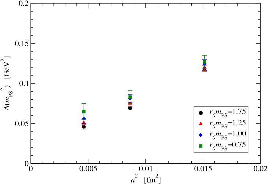
Figure 3: The difference between charged and neutral squared pseudoscalar meson masses as a function of squared lattice spacing, for selected values of the charged meson mass.

Fig. 3 shows the lattice spacing dependence of the squared mass differences for four mass values that span the range of our available data. At leading-order in tm$\chi$PT, Eq. (39) indicates that this quantity should be independent of mass, linear in $a^{2}$ and vanishing in the continuum limit. Modulo the unknown higher order effects, Fig. 3 is in reasonable agreement with these expectations. In particular, the approximate mass independence is evident and the dependence on $a^{2}$ is approximately linear, though a linear fit misses the massless prediction at $a=0$ by a few (statistical) standard deviations.

It should be noted from Fig. 3 that even at our smallest lattice spacing, the mass splitting of $m_{K^{0}}-m_{K^{\pm}}\sim 50$ MeV is significant relative to the kaon mass itself. However, in terms of the difference of mass squared, our results are consistent with the pseudoscalar meson mass splittings in Ref. flavorbreaking and compatible with the suggestion of ShindlerShindler that flavor breaking effects in tmLQCD are of a magnitude comparable to “taste” symmetry violations in pseudoscalar meson masses observed with improved staggered fermionsAubin . The appearance of sizable lattice spacing effects like this have led some authors to use a power counting scheme in which $O(a^{2})$ effects are taken to be LO rather than NLOAoki ; AokiBar2005 , but we will follow Eq. (7) throughout the present work.

The decay constant of a charged pseudoscalar meson can be obtained easily from the so-called indirect methodFrezSint ; Bietenholz ,

$$f_{\rm PS}=\left.\left.\frac{\mu_{l,\,0}+\mu_{h,\,0}}{m_{\rm PS}^{2}}\right|\left<0|\bar{s}\gamma_{5}u|K^{+}\right>\right|.$$ (46)

where the normalization is such that $f_{\pi}\approx 130$ MeV, i.e. larger than the normalization from our tm$\chi$PT conventions by $\sqrt{2}$. Unfortunately, the indirect method does not provide easy access to the neutral pseudoscalar decay constant, due to mixing with the scalar operator. The neutral decay constant is not directly accessible in the laboratory due to the absence of flavor-changing neutral currents in the standard model, but it is a quantity that appears in the parametrization of some neutral kaon matrix elements (see Ref. dimop for a very recent example in the context of tmLQCD). From the point of view of our work, the comparison of charged and neutral cases would be able to provide information about how flavor symmetry breaking in tmLQCD affects the structure of mesons. Note that if we had chosen a different convention in Eq. (1), i.e. interchanging the role of $c$ and $s$ quarks as was done in Ref. Pena which focuses on neutral kaons, then the situation would be reversed: the indirect method would have applied to the neutral kaon and not to the charged kaon.

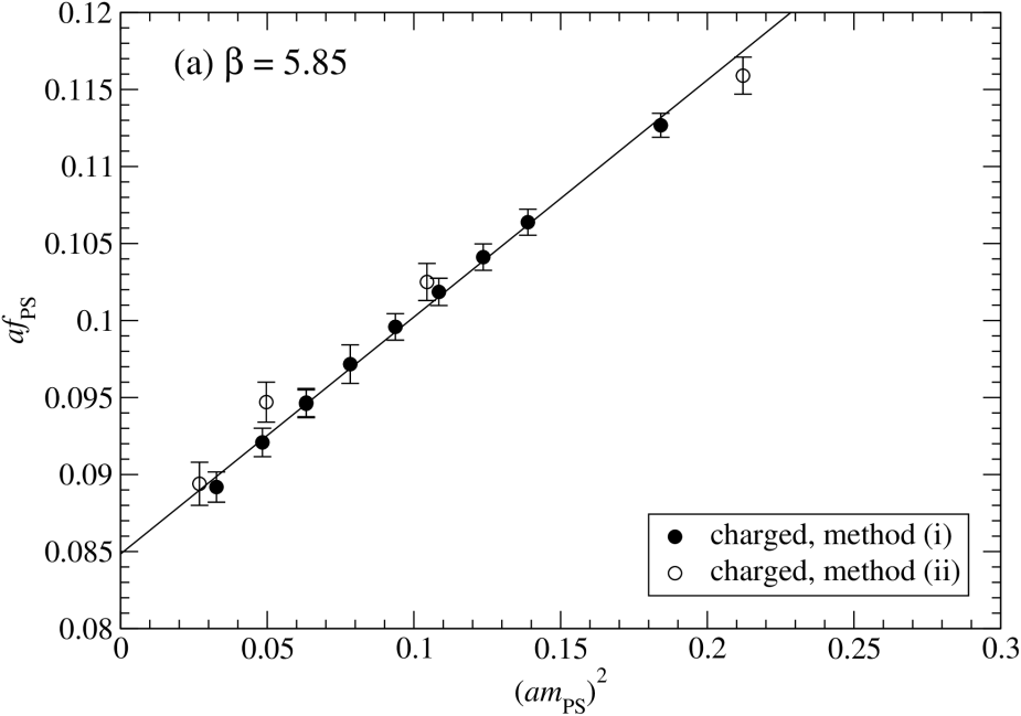
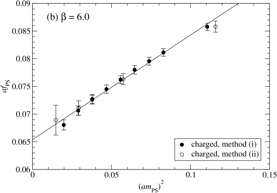
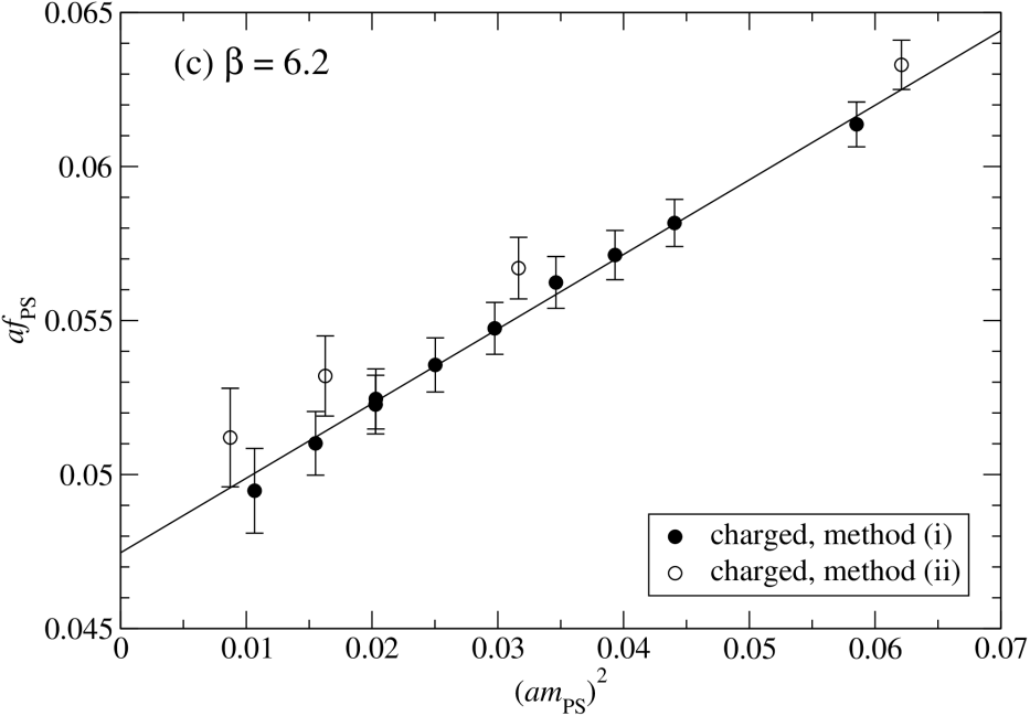
Figure 4: The pseudoscalar meson decay constant as a function of the squared charged pseudoscalar meson mass. Results labelled by method (i) are from the present work; results labelled by method (ii) are from Ref. scaling . Straight lines are linear fits to the data from method (i).

The charged kaon decay constant is plotted in Fig. 4 where we continue to define this meson to be the ground state pseudoscalar meson containing one $s$ (anti)quark from the heavy doublet and one $u$ (anti)quark from the light doublet. Central values show a hint of curvature, but within statistical uncertainties the decay constant is linear in the squared meson mass. This is consistent with the tm$\chi$PT expression, i.e. the quenched version of Eq. (III.3) where the slope has no logarithmic corrections. (We have verified that a tm$\chi$PT calculation of the right-hand side of Eq. (46) also yields Eq. (III.3).) The computations of Ref. scaling , using method (ii), also appear in Fig. 4 and are in agreement with the method (i) results.

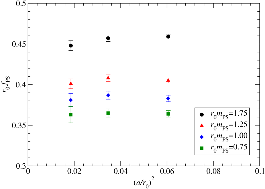
Figure 5: Scaling of the pseudoscalar decay constant for four choices of the quark mass.

As is evident from Fig. 5, there is no visible dependence of the decay constant on lattice spacing. For the kaon, fitting the data from three $\beta$ values linearly yields

$$r_{0}m_{K}=1.25\qquad\Rightarrow\qquad f_{K}=161\pm 5{\rm~{}MeV}\,.$$ (47)

Relying on a linear chiral extrapolation, we similarly obtain

$$f_{\pi}=142\pm 4{\rm~{}MeV}\,.$$ (48)

The ratio,

$$\frac{f_{K}}{f_{\pi}}=1.136(7)\,,$$ (49)

agrees nicely with the quenched results from Ref. CPPACS , though the individual decay constants are somewhat larger. Using the lattice spacings derived from Ref. Gockeler or Dong would bring us into closer agreement.

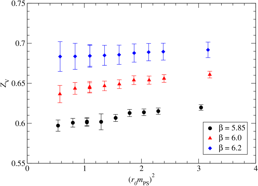
Figure 6: The renormalization factor associated with the pseudoscalar meson decay constant.

There is also a direct methodBietenholz for obtaining the decay constant, though it requires input of a renormalization factor for the twisted vector current. Here, we will use the ratio of results from the direct and indirect methods to determine this renormalization factor. Figure 6 shows that the renormalization factor is essentially mass-independent and that it becomes closer to unity as $a\to 0$. The numerical values are comparable to those obtained by the authors of Ref. scaling , and those authors also note that $Z_{V}$ is further from unity in tmLQCD than in both standard and boosted lattice perturbation theory. (See their Table 7.)

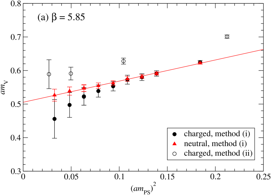
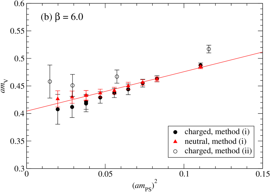
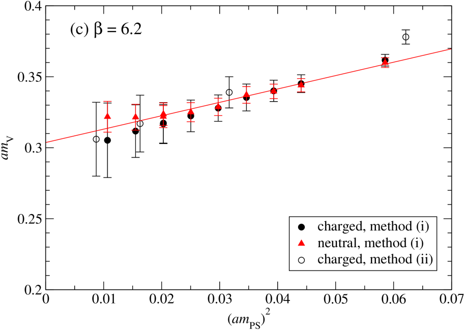
Figure 7: Vector meson mass as a function of the squared charged pseudoscalar meson mass. Results labelled by method (i) are from the present work; results labelled by method (ii) are from Ref. scaling . Straight lines are linear fits to the neutral data from method (i).

Vector meson masses, referred to here as $K^{*}$ masses since the strange (anti)quark from the heavy doublet is combined with a $u$ or $d$ (anti)quark from the light doublet, are shown in Fig. 7, as computed from local operators of the form $\sum_{k=1}^{3}\bar{\psi}\gamma_{k}\psi$. Within the statistical uncertainties, no mass splitting is visible between charged and neutral vector mesons. Comparison with data from the $\chi$LF collaboration reveals that methods (i) and (ii) lead to different $K^{*}$ masses on coarser lattices, and that the distinction vanishes as $a\to 0$. The sizable uncertainties make chiral extrapolations difficult, particularly for charged mesons. Linear fits to the neutral meson masses at each $\beta$ are displayed in Fig. 7.

It is noteworthy that the neutral $K^{*}$ masses are more precise than the charged $K^{*}$, just as the charged pseudoscalar masses are more precise than the neutral pseudoscalar. In both cases, the better precision comes in the channel where the interpolating fields are invariant under twisting. Moreover, the absence of large cutoff effects for charged pseudoscalars has been associated with the existence of an exact lattice axial Ward-Takahashi identity.FMPRcutoff

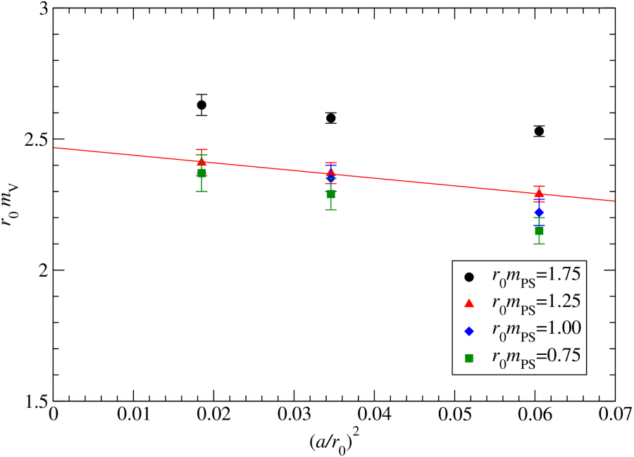
Figure 8: Scaling of the neutral vector meson mass for four choices of the quark mass. The straight line is a linear fit to the data having $r_{0}m_{\rm PS}=1.25$.

Scaling of the neutral vector meson mass with $a^{2}$ is shown in Fig. 8. The nonvanishing dependence on $a^{2}$ is barely significant with respect to the uncertainties. A linear $a^{2}$ fit to the $r_{0}m_{\rm PS}=1.25$ data produces

$$m_{K^{*}}=970\pm 20{\rm~{}MeV}\,,$$ (50)

and a linear $a^{2}$ fit to the linear chiral extrapolations from Fig. 7 yields

$$m_{\rho}=916\pm 20{\rm~{}MeV}\,.$$ (51)

These quenched values lie above the physical values, but using the lattice spacings derived from Ref. Gockeler or Dong would bring us closer to experiment.

VI Scalar meson masses and mixings

Our chosen definition of maximal twist, Eq. (32), tunes the mixing of vector and axial currents for charged mesons, or more precisely, for mesons built from a quark and antiquark having twist angles of opposite sign. Charged scalar and pseudoscalar densities do not mix. Conversely, there is mixing of neutral scalar and pseudoscalar densities, while neutral vector and axial currents do not mix. Our charged vector-axial tuning to maximal twist can differ from a neutral scalar-pseudoscalar definition, for example by differing discretization effects.

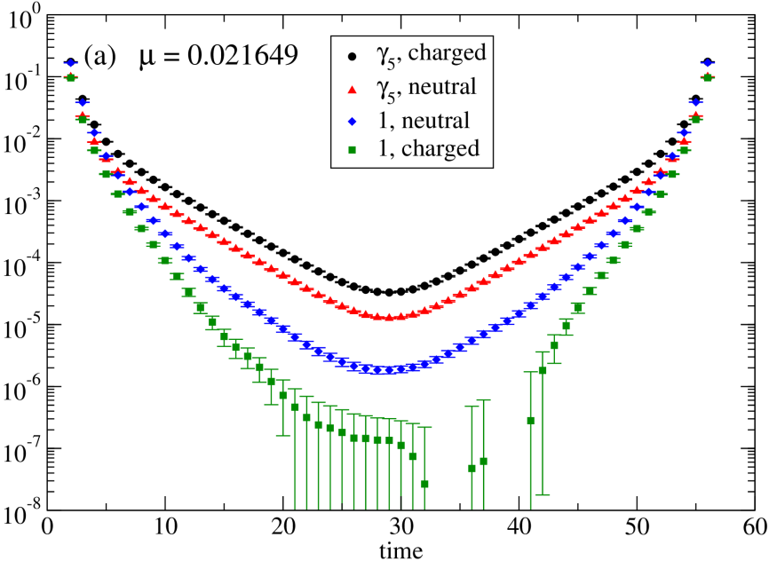
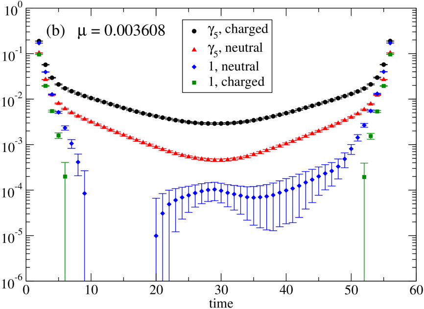
Figure 9: Scalar and pseudoscalar correlation functions for our (a) heaviest and (b) lightest quarks at $\beta=6.2$. The notation $\gamma_{5}$ and $1$ refers to the physical basis, defined using method (i).

Figure 9(a) shows four correlators at $\beta=6.2$ with our heaviest quark mass: charged and neutral scalar and pseudoscalar two-point correlators. The charged correlators cannot mix, and we see a clear ground state exponential behavior for the pseudoscalar and scalar mesons, with no contamination between them. The neutral pseudoscalar correlator also provides a clear ground state, where the slope in this log plot is slightly steeper than the charged case, as expected since we have already established that the neutral meson is heavier than the charged meson. The neutral scalar correlator is noticeably different: it maintains surprisingly small error bars even far from the source, it displays a kink (change of slope on the log plot) near timesteps 12 and 46, and it mirrors the neutral pseudoscalar curve between these timesteps. Apparently the quickly-decaying scalar signal is being overcome by the pseudoscalar further from the source, i.e. we are seeing scalar-pseudoscalar mixing.

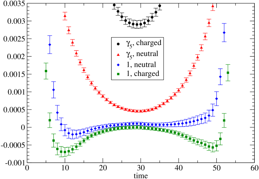
Figure 10: The data from Fig. 9 (b), replotted on a linear scale.

Figure 9(b) shows the same four correlators but now with our lightest quark mass. The effects are now more dramatic, and a new phenomenon is also observed. The charged scalar has a brief signal for the scalar meson near the source, then the correlator becomes negative. The neutral scalar similarly has a brief signal, then makes a curious waving shape on the graph. To understand this, see Fig. 10 where the data from Fig. 9(b) are replotted on a linear scale. The negative contribution to the charged scalar correlator is from the two particle state — quenched $\eta^{\prime}$ and kaon — as discussed in Refs. Bardeen ; Kentucky . The neutral scalar has this two particle state as well, but the correlator is deformed because it apparently also has a mixing with the neutral pseudoscalar.

One could imagine removing the scalar-pseudoscalar mixing by tuning to maximal twist directly in this sector, called method (iii) in the notation of Ref. Sharpe , but mixing could then arise between vector and axial currents. An interesting observation, sketched in Fig. 1 of Ref. Sharpe , is that method (iii) is distinct from method (i) but identical to method (ii) up to $O(a^{2})$ corrections. Could method (ii) be optimal for both the vector-axial and the scalar-pseudoscalar sectors?

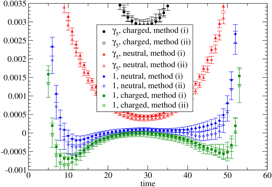
Figure 11: The data from Fig. 10, compared to computations using method (ii).

We have computed 100 quark propagators using method (ii) at $\beta=6.2$ and $\mu_{l,\,0}=0.003608$, allowing a direct comparison to our results from method (i). The method (ii) value of normal quark mass, $m_{l,\,0}=-0.741546$, was obtained from Table 3 in Ref. flavorbreaking . Our findings are displayed in Fig. 11, and we see that the scalar-pseudoscalar mixing is still apparent, confirming the presence of $O(a^{2})$ effects.

VII Untwisted strange with twisted up and down quarks

If the twist angle, $\omega_{h}$, of the heavy doublet is set to zero, then the strange quark becomes a standard Wilson fermion and its partner can be erased from the action. Exceptional configurations are typically not a problem for strange quarks, and $O(a)$ improvement could be accomplished via a Sheikholeslami-Wohlert term if desired, though we will use the unimproved Wilson action here. The $(u,d)$ doublet will be kept at maximal twist.

With this action, the $K^{+}$ and $\bar{K}^{0}$ mesons are exactly degenerate configuration by configuration since one correlator is the Hermitian conjugate of the other. The same is true for $K^{-}$ and $K^{0}$. Furthermore, these two pairs are numerically degenerate in the configuration average. This can easily be seen in the free quark limit, since the twisted mass in one propagator cannot contribute to the correlator if the other propagator is Wilson, due to the odd number of $\gamma_{5}$’s. Similarly, our tm$\chi$PT expression for the mass difference, Eq. (39), explicitly vanishes when $\omega_{h}=0$.

Numerical results at $\beta=6.0$ for kaon masses obtained with a Wilson strange quark are compared to results with a maximally-twisted strange quark in Fig. 12. For this plot, the twisted strange quark is held fixed at $a\mu_{h,\,0}=0.030$ and the Wilson strange quark’s hopping parameter, $\kappa$, is tuned such that the pseudoscalar mass (obtained from two Wilson propagators without any twisting) becomes numerically equal to the charged twisted pseudoscalar mass, $am_{\rm PS}=0.332(1)$. The resulting hopping parameter is $\kappa=0.1545$ or equivalently $m_{h,\,0}=-0.7634$. In both cases, the light quark takes on all four $(m_{l,\,0},\mu_{l,\,0})$ values from Table 1.

Fig. 12 shows that the Wilson strange quark leads to kaon masses that are numerically between the charged and neutral kaons with a twisted strange quark. All curves are visibly linear in $a\mu_{l,\,0}$, though the Wilson strange quark theory has a smaller slope than the twisted strange quark theory. Recall that method (i), used here, itself has a smaller slope than method (ii).

Untwisting the strange quark has other effects besides eliminating the mass splitting. When an untwisted quark field is combined with a maximally twisted one, parity violation induces parity mixing in all (charged and neutral) channels (this can be inferred from Eq (III.2)). This is unlike the situation with complete maximal twisting where in some channels the parity violation in the action interchanges parity of the correlator but does not mix it. With an untwisted strange quark the extraction of the decay constant becomes a much more difficult problem which is beyond the scope of the present work.

VIII Summary

Twisted mass lattice QCD is a practical method for numerical simulations involving light quarks. It has no exceptional configurations, automatic $O(a)$ improvement, and a corresponding version of chiral perturbation theory. However, there are issues of parity and flavor symmetry violation effects at non-zero lattice spacing that have to be understood and dealt with.

Quarks come in pairs in tmLQCD, so the best way to implement three-flavor simulations requires thought and exploration. In this work, we have considered two doublets at maximal twist, where in our quenched simulations the fourth quark is benign. This is in line with the two-doublet tmLQCD proposed in Ref. Pena . The chiral perturbation theory is formulated as a natural generalization of the existing two-flavor formulation, and used to obtain analytic expressions for masses and decay constants. Numerical tmLQCD results for $m_{\pi}$, $f_{\pi}$, $m_{K}$, $f_{K}$, $m_{\rho}$ and $m_{K^{*}}$ are obtained from four twisted quark masses at each of three lattice spacings, and are comparable to previous quenched studies with other actions.

Though dynamical simulations were not performed in this study, that is certainly an ultimate goal for QCD phenomenology. Dynamical simulations of the theory with two twisted doublets would mean the fourth quark is no longer benign. Identifying it with the physical charm quark requires the introduction of a mass splitting within the heavy doublet. Progress toward two-doublet dynamical twisted mass simulations is reviewed in Ref. Farchioni05 . Alternatively, one could avoid an active charm quark by using a mixed action formalismmixedaction , for example with twisted $(u,d)$ and untwisted $s$ quarks in the sea (recall Sec. VII), and Eq. (2) used for the valence quarks (so the strange quark’s partner is again benign).

One of the significant twist artifacts found in this work is the mass difference between charged and neutral kaons, which vanishes in the continuum limit but remains sizable at the lattice spacings studied here, $0.068$ fm $<a<0.123$ fm. This splitting depends upon the particular action that has been chosen; it may be different in other variants of tmLQCD or in nonquenched simulations. For example, if only the up and down quarks, not the strange quark, are twisted, then this large splitting vanishes however at the price of a more complicated pattern of parity mixing in the correlators. $O(a)$ errors also arise in that scenario, though these could be removed by the addition of a suitable clover operator.

Another artifact of twisting is the mixing of scalar and pseudoscalar operators when the standard definitions of maximal twist are employed. For sufficiently light quarks in the quenched approximation, this can be studied through the appearance of negative correlators that correspond to the opening of a quenched $\eta^{\prime}K$ channel.

Notwithstanding the existence of twisted lattice artifacts, we see value in the general approach of tmLQCD for applications involving $u$, $d$ and $s$ quarks. There are a number of options for constructing the action including strange quarks, and with systematic studies such as this one exploring them we can be hopeful that an optimal approach will be found.

Appendix A Currents and densities in the twisted basis

With the generators of $SU(2)$ replaced by those of $SU(4)$, the currents and densities in the twisted basis of the two-doublet theory are defined in the same way as for the one-doublet theorySW04 . At LO, the currents and densities have the same form, mutatis mutandis, as in the $SU(2)$ theory. In the physical basis, i.e. in terms of the physical variable $\Sigma_{ph}$, they take the forms (with a “hat” denoting the physical basis quantity),

$$V^{a}_{\mu,\,LO}=\cos(\Delta^{a}\omega_{m})\hat{V}^{a}_{\mu,\,LO}-\eta_{ab}\sin(\Delta^{a}\omega_{m})\hat{A}^{b}_{\mu,\,LO}\,,\qquad V^{3,\,8,\,15}_{\mu,\,LO}=\hat{V}^{3,\,8,\,15}_{\mu,\,LO}\,,$$

$$A^{a}_{\mu,\,LO}=\cos(\Delta^{a}\omega_{m})\hat{A}^{a}_{\mu,\,LO}-\eta_{ab}\sin(\Delta^{a}\omega_{m})\hat{V}^{b}_{\mu,\,LO}\,,\qquad A^{3,\,8,\,15}_{\mu,\,LO}=\hat{A}^{3,\,8,\,15}_{\mu,\,LO}\,,$$

$$S^{0}_{LO}=\frac{1}{2}(c_{l,\,m}+c_{h,\,m})\hat{S}^{0}_{LO}-2is_{l,\,m}\hat{P}^{3}_{LO}$$

$$\qquad\;\;\;+2(c_{l,\,m}-c_{h,\,m})\left(\frac{1}{\sqrt{3}}\hat{S}^{8}_{LO}+\frac{1}{\sqrt{6}}\hat{S}^{15}_{LO}\right)-2is_{h,\,m}\left(\frac{1}{\sqrt{3}}\hat{P}^{8}_{LO}-\sqrt{\frac{2}{3}}\hat{P}^{15}_{LO}\right)\,,$$

$$S^{a}_{LO}=\cos(\Sigma^{a}\omega_{m})\hat{S}^{a}_{LO}-i\sin(\Sigma^{a}\omega_{m})\hat{P}^{a}_{LO}\,,\qquad P^{a}_{LO}=\cos(\Sigma^{a}\omega_{m})\hat{P}^{a}_{LO}-i\sin(\Sigma^{a}\omega_{m})\hat{S}^{a}_{LO}\,,$$

$$a,\,b\in\mathfrak{K}\backslash\mathfrak{D}\,,\qquad\mathfrak{K}=\{1,\ldots,15\}\,,\qquad\mathfrak{D}=\{3,\,8,\,15\}\,,$$ (52)

where $c_{p,\,m}=\cos\omega_{p,\,m}$, $s_{p,\,m}=\sin\omega_{p,\,m}$, $p=l,\,h$, and we use the notation defined in Eqs. (28-30). Note that in the $SU(4)$ theory, $P^{0}_{LO}$ and $S^{k}_{LO}$, $k\in\mathfrak{K}$, do not vanish identically in contrast to the $SU(2)$ theorySW05 .

At NLO, the vector and axial currents are given by

$$V^{k}_{\mu} =V^{k}_{\mu,\,LO}\,(1+\mathcal{C})+L_{1,\,2,\,3,\,9}\,\mathrm{terms}$$

$$\quad+L_{5}\,\frac{1}{2}\mathrm{Tr}\Big{[}\Big{(}[\Lambda_{k},\Sigma]_{-}\,\partial_{\mu}\Sigma^{\dagger}-\partial_{\mu}\Sigma\,[\Lambda_{k},\Sigma]_{-}\Big{)}(\chi^{\prime}\Sigma^{\dagger}+\Sigma\chi^{\prime\dagger})\Big{]}$$

$$\quad+\widetilde{W}_{5}\,\frac{1}{2}\mathrm{Tr}\Big{[}\Big{(}[\Lambda_{k},\Sigma]_{-}\,\partial_{\mu}\Sigma^{\dagger}-\partial_{\mu}\Sigma\,[\Lambda_{k},\Sigma]_{-}\Big{)}(\hat{A}\Sigma^{\dagger}+\Sigma\hat{A}^{\dagger})\Big{]}\,,$$

$$A^{k}_{\mu} =A^{k}_{\mu,\,LO}\,(1+\mathcal{C})+\frac{8aW_{0}}{B_{0}f^{2}}W_{10}\,\partial_{\mu}P^{k}_{LO}+L_{1,\,2,\,3,\,9}\,\mathrm{terms}$$

$$\quad-L_{5}\,\frac{1}{2}\mathrm{Tr}\Big{[}\Big{(}[\Lambda_{k},\Sigma]_{+}\,\partial_{\mu}\Sigma^{\dagger}-\partial_{\mu}\Sigma\,[\Lambda_{k},\Sigma]_{+}\Big{)}(\chi^{\prime}\Sigma^{\dagger}+\Sigma\chi^{\prime\dagger})\Big{]}$$

$$\quad-\widetilde{W}_{5}\,\frac{1}{2}\mathrm{Tr}\Big{[}\Big{(}[\Lambda_{k},\Sigma]_{+}\,\partial_{\mu}\Sigma^{\dagger}-\partial_{\mu}\Sigma\,[\Lambda_{k},\Sigma]_{+}\Big{)}(\hat{A}\Sigma^{\dagger}+\Sigma\hat{A}^{\dagger})\Big{]}\,,$$ (53)

where $k\in\mathfrak{K}$, and

$$\mathcal{C} =\frac{4L_{4}}{f^{2}}\,\mathrm{Tr}[\chi^{\prime\dagger}\Sigma+\Sigma^{\dagger}\chi^{\prime}]+\frac{4\widetilde{W}_{4}}{f^{2}}\mathrm{Tr}(\hat{A}^{\dagger}\Sigma+\Sigma^{\dagger}\hat{A})$$ (54)

We do not give the form of the $L_{1,\,2,\,3,\,9}$ terms since each has the same form as in the continuum $SU(2)$ theoryGL84 .

Dropping terms proportional to the scalar and pseudoscalar sources, which give rise only to contact terms in correlation functions, the scalar and pseudoscalar densities at NLO are given by

$$S^{k} =S^{k}_{LO}\,(1+\mathcal{D}_{1})+P^{k}_{LO}\,\mathcal{D}_{2}+L_{5}\,B_{0}\mathrm{Tr}\big{[}\partial_{\mu}\Sigma\partial_{\mu}\Sigma^{\dagger}(\Lambda_{k}\Sigma^{\dagger}+\Sigma\Lambda_{k})\big{]}$$

$$\quad-L_{8}\,2B_{0}\mathrm{Tr}\big{[}(\Lambda_{k}\Sigma^{\dagger}+\Sigma\Lambda_{k})(\chi^{\prime}\Sigma^{\dagger}+\Sigma\chi^{\prime\dagger})\big{]}-\widetilde{W}_{8}\,B_{0}\mathrm{Tr}\big{[}(\Lambda_{k}\Sigma^{\dagger}+\Sigma\Lambda_{k})(\hat{A}\Sigma^{\dagger}+\Sigma\hat{A}^{\dagger})\big{]}\,,$$

$$P^{k} =P^{k}_{LO}\,(1+\mathcal{D}_{1})+S^{k}_{LO}\,\mathcal{D}_{2}+L_{5}\,B_{0}\mathrm{Tr}\big{[}\partial_{\mu}\Sigma\partial_{\mu}\Sigma^{\dagger}(\Lambda_{k}\Sigma^{\dagger}-\Sigma\Lambda_{k})\big{]}$$

$$\quad-L_{8}\,2B_{0}\mathrm{Tr}\big{[}(\Lambda_{k}\Sigma^{\dagger}-\Sigma\Lambda_{k})(\chi^{\prime}\Sigma^{\dagger}+\Sigma\chi^{\prime\dagger})\big{]}-\widetilde{W}_{8}\,B_{0}\mathrm{Tr}\big{[}(\Lambda_{k}\Sigma^{\dagger}-\Sigma\Lambda_{k})(\hat{A}\Sigma^{\dagger}+\Sigma\hat{A}^{\dagger})\big{]}\,,$$

$$\quad+4iH_{2}B_{0}^{2}\mathrm{Tr}(\Lambda_{k}\boldsymbol{\mu})\,,$$ (55)

where $k\in\mathfrak{K}$, and

$$\mathcal{D}_{1} =-\frac{4L_{4}}{f^{2}}\,\mathrm{Tr}[D_{\mu}\Sigma D_{\mu}\Sigma^{\dagger}]+\frac{8L_{6}}{f^{2}}\,\mathrm{Tr}(\chi^{\prime\dagger}\Sigma+\Sigma^{\dagger}\chi)+\frac{4\widetilde{W}_{6}}{f^{2}}\mathrm{Tr}(\hat{A}^{\dagger}\Sigma+\Sigma^{\dagger}\hat{A})\,,$$

$$\mathcal{D}_{2} =-\frac{8L_{7}}{f^{2}}\mathrm{Tr}(\chi^{\prime\dagger}\Sigma-\Sigma^{\dagger}\chi^{\prime})-\frac{4\widetilde{W}_{7}}{f^{2}}\mathrm{Tr}(\hat{A}^{\dagger}\Sigma-\Sigma^{\dagger}\hat{A})\,.$$ (56)

To write the NLO currents and densities in the physical basis, we need the results

$$\mathrm{Tr}(D_{\mu}^{\dagger}\Sigma D_{\mu}\Sigma^{\dagger})=\mathrm{Tr}(D_{\mu}^{\dagger}\Sigma_{ph}D_{\mu}\Sigma_{ph}^{\dagger})\,,$$

$$\mathrm{Tr}(\chi^{\prime\dagger}\Sigma\pm\Sigma^{\dagger}\chi)=\begin{cases}-\frac{4\hat{M}^{\prime}}{2B_{0}f^{2}}\hat{S}^{0}_{LO}-\frac{4\Delta M^{\prime}}{B_{0}f^{2}}(\frac{1}{\sqrt{3}}\hat{S}^{8}_{LO}+\frac{1}{\sqrt{6}}\hat{S}^{15}_{LO})\quad(+\;\mathrm{sign})\\ \quad\!\frac{4\hat{M}^{\prime}}{2B_{0}f^{2}}\hat{P}^{0}_{LO}+\frac{4\Delta M^{\prime}}{B_{0}f^{2}}(\frac{1}{\sqrt{3}}\hat{P}^{8}_{LO}+\frac{1}{\sqrt{6}}\hat{P}^{15}_{LO})\quad(-\;\mathrm{sign})\end{cases}+O(M_{p}^{\prime}\epsilon_{p})\,,$$

$$\mathrm{Tr}(\hat{A}^{\dagger}\Sigma\pm\Sigma^{\dagger}\hat{A})=\begin{cases}-\frac{8W_{0}a}{2B_{0}f^{2}}\hat{S}^{0}_{LO}\quad(+\;\mathrm{sign})\\ \quad\!\frac{8W_{0}a}{2B_{0}f^{2}}\hat{P}^{0}_{LO}\quad(-\;\mathrm{sign})\end{cases}+O(a\epsilon_{p})\,,\qquad p=l,\,h\,,$$ (57)

where

$$\hat{M}^{\prime}\equiv(M_{l}^{\prime}+M_{h}^{\prime})/2\,,\qquad\Delta M^{\prime}\equiv M_{l}^{\prime}-M_{h}^{\prime}\,,$$ (58)

which allow us to express $\mathcal{C}$, $\mathcal{D}_{1}$, and $\mathcal{D}_{2}^{\pm}$ in terms of the physical fields.

Next we write the $L_{5}$, $L_{8}$, $\widetilde{W}_{5}$, $\widetilde{W}_{8}$, and $H_{2}$ terms in the physical basis. For the $L_{5}$ terms, we need the results

$$\pm\frac{1}{2}\mathrm{Tr}\Big{[}\Big{(}[\Lambda_{a},\Sigma]_{\mp}\,\partial_{\mu}\Sigma^{\dagger}-\partial_{\mu}\Sigma\,[\Lambda_{a},\Sigma]_{\mp}\Big{)}(\chi^{\prime}\Sigma^{\dagger}+\Sigma\chi^{\prime\dagger})\Big{]}$$

$$\qquad=\begin{cases}\cos(\Delta^{a}\omega_{m})\hat{V}^{a}_{L_{5}}-\eta_{ab}\sin(\Delta^{a}\omega_{m})\hat{A}^{b}_{L_{5}}\quad(\mathrm{upper\;sign})\\ \cos(\Delta^{a}\omega_{m})\hat{A}^{a}_{L_{5}}-\eta_{ab}\sin(\Delta^{a}\omega_{m})\hat{V}^{b}_{L_{5}}\quad(\mathrm{lower\;sign})\end{cases},$$

$$\mathrm{Tr}\big{[}\partial_{\mu}\Sigma\partial_{\mu}\Sigma^{\dagger}(\Lambda_{a}\Sigma^{\dagger}\pm\Sigma\Lambda_{a})\big{]}=\begin{cases}\cos(\Sigma^{a}\omega_{m})\hat{S}^{a}_{L_{5}}-i\sin(\Sigma^{a}\omega_{m})\hat{P}^{a}_{L_{5}}\quad(+\;\mathrm{sign})\\ \cos(\Sigma^{a}\omega_{m})\hat{P}^{a}_{L_{5}}-i\sin(\Sigma^{a}\omega_{m})\hat{S}^{a}_{L_{5}}\quad(-\;\mathrm{sign})\end{cases},$$ (59)

where $a,\,b\in\mathfrak{K}\backslash\mathfrak{D}$, and

$$\hat{V}^{a}_{L_{5}} =\frac{1}{2}\left\langle\Lambda_{a}\Big{(}\big{[}\Sigma_{ph}\partial\Sigma^{\dagger}_{ph},\chi_{tw}^{\prime}\Sigma^{\dagger}+\Sigma_{ph}\chi_{tw}^{\prime\dagger}\big{]}_{+}+(\Sigma\leftrightarrow\Sigma^{\dagger},\,\chi^{\prime}\leftrightarrow\chi^{\prime\dagger})\Big{)}\right\rangle\,,\qquad\chi_{tw}^{\prime}\equiv\xi_{m}^{\dagger}\chi^{\prime}\xi_{m}^{\dagger}$$

$$\hat{A}^{a}_{L_{5}} =\frac{1}{2}\left\langle\Lambda_{a}\Big{(}\big{[}\Sigma_{ph}^{\dagger}\partial\Sigma_{ph},\chi_{tw}^{\prime\dagger}\Sigma+\Sigma_{ph}^{\dagger}\chi_{tw}^{\prime}\big{]}_{+}-(\Sigma\leftrightarrow\Sigma^{\dagger},\,\chi^{\prime}\leftrightarrow\chi^{\prime\dagger})\Big{)}\right\rangle\,,$$

$$\hat{S}^{a}_{L_{5}} =-\left\langle\Lambda_{a}\big{(}\partial_{\mu}\Sigma_{ph}\Sigma_{ph}^{\dagger}\partial_{\mu}\Sigma_{ph}+\mathrm{h.c.}\big{)}\right\rangle\,,\qquad\hat{P}^{a}_{L_{5}}=\left\langle\Lambda_{a}\big{(}\partial_{\mu}\Sigma_{ph}\Sigma_{ph}^{\dagger}\partial_{\mu}\Sigma_{ph}-\mathrm{h.c.}\big{)}\right\rangle\,,$$ (60)

and for the $L_{8}$ terms we need the results

$$-\mathrm{Tr}\big{[}(\Lambda_{a}\Sigma^{\dagger}\pm\Sigma\Lambda_{a})(\chi^{\prime}\Sigma^{\dagger}+\Sigma\chi^{\prime\dagger})\big{]}=\begin{cases}\cos(\Sigma^{a}\omega_{m})\hat{S}^{a}_{L_{8}}-i\sin(\Sigma^{a}\omega_{m})\hat{P}^{a}_{L_{8}}\quad(+\;\mathrm{sign})\\ \cos(\Sigma^{a}\omega_{m})\hat{P}^{a}_{L_{8}}-i\sin(\Sigma^{a}\omega_{m})\hat{S}^{a}_{L_{8}}\quad(-\;\mathrm{sign})\end{cases},$$

$$\hat{S}^{a}_{L_{8}}=-\left\langle\Lambda_{a}\big{(}\Sigma_{ph}\chi_{tw}^{\prime\dagger}\Sigma_{ph}+\mathrm{h.c.}\big{)}\right\rangle\,,\qquad\hat{P}^{a}_{L_{8}}=\left\langle\Lambda_{a}\big{(}\Sigma_{ph}\chi_{tw}^{\prime\dagger}\Sigma_{ph}-\mathrm{h.c.}\big{)}\right\rangle\,,\qquad a\in\mathfrak{K}\backslash\mathfrak{D}\,.$$ (61)

By replacing $\chi^{\prime}$ with $\hat{A}$, and $L_{5,\,8}$ with $\widetilde{W}_{5,\,8}$, the $\widetilde{W}_{5}$ and $\widetilde{W}_{8}$ terms can be expressed in the physical basis using the same results above for the $L_{5}$ and $L_{8}$ terms.

Lastly, the $H_{2}$ term contributes only in the flavor-diagonal case, i.e. when the flavor index $k=3,\,8,\,15$. Since we will not be using the flavor-diagonal currents and densities, we do not give results for the flavor-diagonal cases here.

To conclude this appendix, we provide the explicit expression for the axial current in the physics basis at NLO, using the twist angles determined in Sec. III.2:

$$\hat{A}^{a}_{\mu} =\hat{A}^{a}_{\mu,\,LO}-\frac{8W_{0}a}{f^{2}}W_{10}\cos(\Sigma^{a}\omega_{m})\sin(\Delta^{a}\omega_{m})\eta_{ab}\hat{V}^{b}_{\mu,\,LO}(1+\mathcal{C})+L_{1,\,2,\,3,\,9}\,\mathrm{terms}$$

$$\quad+\frac{8W_{0}a}{B_{0}f^{2}}W_{10}\cos(\Delta^{a}\omega_{m})\Big{[}\cos(\Sigma^{a}\omega_{m})\partial_{\mu}\hat{P}^{a}_{LO}-i\sin(\Sigma^{a}\omega_{m})\partial_{\mu}\hat{S}^{a}_{LO}\Big{]}$$

$$\quad+L_{5}\bigg{[}\hat{A}^{a}_{L_{5}}-\frac{8W_{0}a}{f^{2}}W_{10}\cos(\Sigma^{a}\omega_{m})\sin(\Delta^{a}\omega_{m})\eta_{ab}\hat{V}^{b}_{L_{5}}\bigg{]}+\big{[}L_{5}\leftrightarrow\widetilde{W}_{5}\big{]}\,.$$ (62)

The term $\mathcal{C}$ is the same as in Eq. (54), but now given in the physical basis.

Table 1: The parameters used for simulations in this work. Lattice spacings are taken from Ref. Jansen1 . Each $(am_{p,\,0},a\mu_{p,\,0})$ pair is the result of tuning to maximal twist with method (i) as discussed in Sec. IV. The subscript $p=l,h$ is used in the text to distinguish the “light” quark doublet from the “heavy” quark doublet, but for purposes of numerical tuning in this table there is no distinction. The twist angle was obtained from Eq. (41).

$\beta$	$a$ [fm]	#sites	#configurations	$am_{p,\,0}$	$a\mu_{p,\,0}$	twist angle (degrees)
5.85	0.123	$20^{3}\times 40$	600	-0.8965	0.0376	90.0$\pm$	0.3
				-0.9071	0.0188	90.2$\pm$	0.6
				-0.9110	0.01252	90.6$\pm$	0.8
				-0.9150	0.00627	90.6$\pm$	1.6
6.0	0.093	$20^{3}\times 48$	600	-0.8110	0.030	90.4$\pm$	0.4
				-0.8170	0.015	91.0$\pm$	0.7
				-0.8195	0.010	92.5$\pm$	1.0
				-0.8210	0.005	95.5$\pm$	2.1
6.2	0.068	$28^{3}\times 56$	200	-0.7337	0.021649	89.1$\pm$	0.8
				-0.7367	0.010825	87.3$\pm$	1.8
				-0.7378	0.007216	86.3$\pm$	2.8
				-0.7389	0.003608	86.4$\pm$	4.5

Table 2: Numerical values from our simulations. These are also shown graphically in the figures. The rows with superscripts $a$ and $b$ refer to ($a\mu_{h,0}$,$a\mu_{l,0}$)=(0.015,0.005) and (0.010,0.010) respectively.

$\beta$	$a\mu_{l,\,0}+a\mu_{h,\,0}$	$(am_{\rm PS})^{2}$		$af_{\rm PS}$	$Z_{V}$	$am_{V}$
		charged	neutral			charged	neutral
5.85	0.0752	0.1841(4)	0.2262(12)	0.1127(8)	0.620(4)	0.625(5)	0.622(3)
	0.0564	0.1388(4)	0.1827(14)	0.1064(8)	0.615(4)	0.591(8)	0.591(5)
	0.05012	0.1236(4)	0.1683(15)	0.1041(9)	0.614(4)	0.580(10)	0.582(6)
	0.04387	0.1085(4)	0.1536(19)	0.1019(9)	0.613(4)	0.573(13)	0.575(8)
	0.0376	0.0937(3)	0.1402(15)	0.0996(9)	0.607(4)	0.553(14)	0.563(7)
	0.03132	0.0784(10)	0.1259(16)	0.0972(13)	0.602(10)	0.539(18)	0.555(9)
	0.02507	0.0633(3)	0.1112(19)	0.0947(9)	0.602(5)	0.523(26)	0.548(10)
	0.02504	0.0633(3)	0.1117(17)	0.0946(9)	0.601(5)	0.522(25)	0.547(10)
	0.01879	0.0484(2)	0.0969(22)	0.0921(9)	0.601(5)	0.497(37)	0.539(12)
	0.01254	0.0327(2)	0.0824(33)	0.0892(10)	0.597(7)	0.456(58)	0.527(18)
6.0	0.060	0.1106(4)	0.1260(6)	0.0858(7)	0.661(4)	0.488(4)	0.484(3)
	0.045	0.0829(4)	0.0986(7)	0.0811(7)	0.656(5)	0.463(6)	0.462(4)
	0.040	0.0738(4)	0.0898(8)	0.0796(7)	0.654(5)	0.455(7)	0.456(5)
	0.035	0.0646(5)	0.0801(9)	0.0780(8)	0.654(6)	0.444(10)	0.450(7)
	0.030	0.0558(4)	0.0724(7)	0.0762(7)	0.649(5)	0.437(8)	0.441(6)
	0.025	0.0468(4)	0.0641(8)	0.0745(8)	0.647(6)	0.429(10)	0.437(7)
	0.020a	0.0378(4)	0.0550(10)	0.0726(8)	0.646(7)	0.418(15)	0.432(9)
	0.020b	0.0378(4)	0.0559(9)	0.0727(8)	0.644(6)	0.421(14)	0.433(9)
	0.015	0.0290(3)	0.0471(12)	0.0706(8)	0.644(7)	0.412(19)	0.430(11)
	0.010	0.0198(3)	0.0383(18)	0.0680(9)	0.637(11)	0.407(27)	0.426(15)
6.2	0.043298	0.0585(4)	0.0640(6)	0.0614(7)	0.692(10)	0.362(4)	0.360(3)
	0.032474	0.0441(4)	0.0497(6)	0.0582(8)	0.689(11)	0.345(6)	0.344(5)
	0.028865	0.0393(4)	0.0451(7)	0.0571(8)	0.689(11)	0.340(8)	0.340(5)
	0.025257	0.0346(5)	0.0406(7)	0.0562(8)	0.688(11)	0.335(9)	0.337(6)
	0.02165	0.0298(4)	0.0358(7)	0.0547(8)	0.686(12)	0.328(9)	0.329(6)
	0.018041	0.0250(4)	0.0313(7)	0.0536(9)	0.685(13)	0.322(11)	0.325(7)
	0.014433	0.0203(4)	0.0269(8)	0.0525(10)	0.684(13)	0.317(14)	0.324(8)
	0.014432	0.0203(4)	0.0268(8)	0.0523(10)	0.684(14)	0.317(14)	0.322(8)
	0.010824	0.0155(3)	0.0225(9)	0.0510(10)	0.684(16)	0.312(19)	0.321(9)
	0.007216	0.0107(5)	0.0184(11)	0.0495(14)	0.683(19)	0.305(26)	0.322(11)

Figure 12: Squared pseudoscalar meson masses with one strange quark/antiquark and one light quark/antiquark, plotted as a function of the light quark’s twisted mass.

References

- (1) R. Frezzotti, P. A. Grassi, S. Sint and P. Weisz [Alpha collaboration], JHEP 0108, 058 (2001).
- (2) R. Frezzotti and G. C. Rossi, JHEP 0408, 007 (2004).
- (3) A. Shindler, PoS LAT2005, 032 (2005).
- (4) G. Münster and C. Schmidt, Europhys. Lett. 66, 652 (2004).
- (5) G. Münster, JHEP 0409, 035 (2004).
- (6) L. Scorzato, Eur. Phys. J. C 37, 445 (2004).
- (7) S. R. Sharpe and J. M. S. Wu, Phys. Rev. D 70, 094029 (2004).
- (8) S. Aoki and O. Bär, Phys. Rev. D 70, 116011 (2004).
- (9) S. R. Sharpe and J. M. S. Wu, Phys. Rev. D 71, 074501 (2005).
- (10) S. Aoki and O. Bär, PoS LAT2005, 046 (2005).
- (11) S. R. Sharpe, Phys. Rev. D 72, 074510 (2005).
- (12) C. Pena, S. Sint and A. Vladikas, JHEP 0409, 069 (2004).
- (13) F. Farchioni, K. Jansen, I. Montvay, E. Scholz, L. Scorzato, A. Shindler, N. Ukita, C. Urbach and I. Wetzorke, Eur. Phys. J. C 42 73 (2005).
- (14) A. M. Abdel-Rehim, R. Lewis and R. M. Woloshyn, Phys. Rev. D 71, 094505 (2005).
- (15) K. Jansen, A. Shindler, C. Urbach and I. Wetzorke [LF collaboration], Phys. Lett. B 586, 432 (2004).
- (16) F. Farchioni et al., Nucl. Phys. Proc. Suppl. 140, 240 (2005)
- (17) R. Frezzotti and G. C. Rossi, Nucl. Phys. B (Proc. Suppl.) 128, 193 (2004).
- (18) F. Farchioni et al., PoS LAT2005, 072 (2005).
- (19) P. Dimopoulos, J. Heitger, F. Palombi, C. Pena, S. Sint and A. Vladikas, hep-ph/0601002.
- (20) R. Frezzotti and G. C. Rossi, JHEP 0410, 070 (2004)
- (21) G. Rupak and N. Shoresh, Phys. Rev. D 66, 054503 (2002).
- (22) O. Bar, G. Rupak and N. Shoresh, Phys. Rev. D 70, 034508 (2004).
- (23) O. Bar, G. Rupak and N. Shoresh, Phys. Rev. D 67, 114505 (2003).
- (24) S. Sharpe and R. Singleton, Jr, Phys. Rev. D 58, 074501 (1998).
- (25) J. Gasser and H. Leutwyler, Nucl. Phys. B 250, 465 (1985).
- (26) A. M. Abdel-Rehim, R. Lewis and R. M. Woloshyn, PoS LAT2005, 051 (2005).
- (27) K. Jansen, C. McNeile, C. Michael, K. Nagai, M. Papinutto, J. Pickavance, A. Shindler, C. Urbach and I. Wetzorke, hep-lat/0507032.
- (28) K. Jansen, M. Papinutto, A. Shindler, C. Urbach and I. Wetzorke, JHEP 0509, 071 (2005).
- (29) S. R. Sharpe, Phys. Rev. D 46, 3146 (1992).
- (30) C. W. Bernard and M. F. L. Golterman, Phys. Rev. D 46, 853 (1992).
- (31) S. Aoki et al. [CP-PACS collaboration], Phys. Rev. D 67, 034503 (2003).
- (32) M. Gockeler, R. Horsley, H. Perlt, P. Rakow, G. Schierholz, A. Schiller and P. Stephenson, Phys. Rev. D 57, 5562 (1998).
- (33) S. J. Dong, K. F. Liu and A. G. Williams, Phys. Rev. D 58, 074504 (1998).
- (34) C. Aubin et al., Phys. Rev. D 70, 094505 (2004).
- (35) S. Aoki, Phys. Rev. D 68, 054508 (2003).
- (36) R. Frezzotti and S. Sint, Nucl. Phys. B (Proc. Suppl.) 106, 814 (2002).
- (37) W. Bietenholz et al. [LF collaboration], JHEP 0412, 044 (2004).
- (38) R. Frezzotti, G. Martinelli, M. Papinutto and G. C. Rossi, hep-lat/0503034.
- (39) W. A. Bardeen, A. Duncan, E. Eichten, N. Isgur, H. Thacker, Phys. Rev. D 65, 014509 (2001).
- (40) Y. Chen, S.-J. Dong, T. Draper, I. Horvath, K. F. Liu, N. Mathur, S. Tamhankar, C. Srinivasan, F. X. Lee and J. Zhang, hep-lat/0405001.
- (41) J. Gasser and H. Leutwyler, Annals Phys. 158, 142 (1984).