The spontaneous generation of magnetic fields at high temperature in $SU(2)$-gluodynamics on a lattice

Abstract

The spontaneous generation of the chromomagnetic field at high temperature is investigated in a lattice formulation of the $SU(2)$-gluodynamics. The procedure of studying this phenomenon is developed. The Monte Carlo simulations of the free energy on the lattices $2\times 8^{3}$, $2\times 16^{3}$ and $4\times 8^{3}$ at various temperatures are carried out. The creation of the field is indicated by means of the $\chi^{2}$-analysis of the data set accumulating 5-10 millions MC configurations. A comparison with the results of other approaches is done.

1 Introduction

Among interesting problems of modern cosmology the origin of large-scale magnetic fields is intensively attacked nowadays. Various mechanisms of the field generation at different stages of the universe evolution were proposed [1]. Basically they are grounded on the idea of Fermi, Chandrasekhar and Zel’dovich that to have the present day galaxy magnetic fields of order $\sim 1\mu G$ correlated on a scale $\sim 1$Mpc seed magnetic fields must be present in the early universe. These fields had been frozen in a cosmic plasma and then amplified by some of the mechanisms of the field amplification. One of the ways to produce seed fields is a spontaneous vacuum magnetization at high temperature $T$ [2, 3, 4, 5]. Actually, this is an extension of the Savvidy model for the QCD vacuum [6], proposed already at $T=0$ and describing the creation of the Abelian chromomagnetic fields due to a vacuum polarization, in case of nonzero temperature. At zero temperature this field configuration is unstable because of the tachyonic mode in the gluon spectrum. At $T\not=0$, the possibility of having strong temperature-dependent and stable magnetic fields was discovered [4]. The field stabilization is ensured by the temperature and field dependent gluon magnetic mass.

Another related field of interest is the deconfinement phase of QCD. As it was realized recently, this is not the gas of free quarks and gluons, but a complicate interacting system of them. This was discovered at RHIC experiments [7] and observed in either perturbative [4, 8] or nonperturbative [9] investigations of the vacuum state with magnetic fields at high temperature. In Refs. [4, 8] the spontaneous creation of the chromomagnetic fields of order $gB\sim g^{4}T^{2}$ was observed in $SU(2)$- and $SU(3)$-gluodynamics within the one-loop plus daisy resummation accounted for. In Ref. [9] the chromomagnetic condensate of same order was obtained in stochastic QCD vacuum model and method of dimensional reduction by comparison with lattice data. In Refs. [10] the response of the vacuum to the influence of strong external fields at different temperatures has been investigated and it was shown that the confinement is restored by increasing the strength of the applied field. These results stimulated the present investigation.

We are going to determine the spontaneous creation of magnetic fields in lattice simulations of $SU(2)$-gluodynamics. In contrast to the problems in the external field, in the case of interest the field strength is a dynamical variable which values at different temperatures have to be determined by means of the minimization of the free energy. This procedure is not a simple one as in continuum because the field strength on a lattice is quantized. To deal with this peculiarity, we consider magnetic fluxes on a lattice as the main objects to be investigated. The fluxes take continuous values, and therefore the minimization of the free energy in presence of magnetic field can be fulfilled in a usual way. These speculations serve as an explanation of the strategy of our calculations.

One of the methods to introduce a magnetic flux on a lattice is to use the twisted boundary conditions (t.b.c.) [11]. In this approach the flux is a continuous quantity. So, in what follows we consider the free energy $F(\varphi)$ with the magnetic flux $\varphi$ on a lattice in the $SU(2)$-gluodynamics and calculate its values at different temperatures by means of Monte Carlo (MC) simulations. We will show that the global minimum of $F(\varphi)$ is located at some non-zero value $\varphi_{min}$ dependent on the temperature. It means the spontaneous creation of the temperature-dependent magnetic fields in the deconfinement phase.

The paper is organized as follows. In sect. 2 some necessary information about the magnetic fluxes on a lattice is adduced. In sect. 3 the calculation details and the results are given. Section 4 is devoted to discussion.

2 Magnetic fields on a lattice

In perturbation theory, the value of the macroscopic (classical) magnetic field generated inside a system is determined by the minimization of the free energy functional. The interaction with the classical field is introduced by splitting the gauge field potential in two parts: $A_{\mu}=\bar{A_{\mu}}+A_{\mu}^{R}$, where $A_{\mu}^{R}$ describes a radiation field and $\bar{A_{\mu}}=(0,0,Hx^{1},0)$ corresponds to the constant magnetic field directed along the third axis. However, on a lattice, the direct detection of the spontaneously generated field strength by straightforward analysis of the configurations, which are produced in the MC simulations, seems to be problematic. Therefore, it is reasonable to follow the approach used in the continuum field theory.

First, let us write down the free energy density,

$$F(\varphi)=-\log\frac{Z(\varphi)}{Z(0)},$$ (1)

$$Z(\varphi)=\int[DU(\varphi)]\exp\{-S(U(\varphi))\}.$$ (2)

Here, $Z(\varphi)$ and $Z(0)$ are the partition function at finite and zero magnetic fluxes, respectively; the link variable $U$ is the lattice analogue of the potential $A_{\mu}$.

The free energy density relates to the effective action as follows,

$$F(\varphi)=\bar{S}(\varphi)-\bar{S}(0),$$ (3)

where $\bar{S}(\varphi)$ and $\bar{S}(0)$ are the effective lattice actions with and without magnetic field, correspondingly.

To detect the spontaneous creation of the field it is necessary to show that the free energy density has the global minimum at a non-zero magnetic flux, $\varphi_{min}\not=0$.

In what follows, we use the hypercubic lattice $L_{t}\times L_{s}^{3}$ ($L_{t}<L_{s}$) with the hypertorus geometry; $L_{t}$ and $L_{s}$ are the temporal and the spatial sizes of the lattice, respectively. In the limit of $L_{s}\to\infty$ the temporal size $L_{t}$ is related to physical temperature. The one-plaquette action of the $SU(2)$ lattice gauge theory can be written as

$$S_{W}=\beta\sum_{x}\sum_{\mu>\nu}\left[1-\frac{1}{2}{\leavevmode\nobreak\ \rm Tr\leavevmode\nobreak\ }U_{\mu\nu}(x)\right];$$ (4)

$$U_{\mu\nu}(x)=U_{\mu}(x)U_{\nu}(x+a\hat{\mu})U_{\mu}^{\dagger}(x+a\hat{\nu})U_{\nu}^{\dagger}(x),$$ (5)

where $\beta=4/g^{2}$ is the lattice coupling constant, $g$ is the bare coupling, $U_{\mu}(x)$ is the link variable located on the link leaving the lattice site $x$ in the $\mu$ direction, $U_{\mu\nu}(x)$ is the ordered product of the link variables.

The effective action $\bar{S}$ in (3) is the Wilson action averaged over the Boltzmann configurations, produced in the MC simulations.

The lattice variable $U_{\mu}(x)$ can be decomposed in terms of the unity, $I$, and Pauli, $\sigma_{j},$ matrices in the color space,

$$U_{\mu}(x)=IU_{\mu}^{0}(x)+i\sigma_{j}U_{\mu}^{j}(x)=\left(\begin{array}[]{cc}U_{\mu}^{0}(x)+iU_{\mu}^{3}(x)&U_{\mu}^{2}(x)+iU_{\mu}^{1}(x)\\ -U_{\mu}^{2}(x)+iU_{\mu}^{1}(x)&U_{\mu}^{0}(x)-iU_{\mu}^{3}(x)\end{array}\right).$$ (8)

The four components $U_{\mu}^{j}(x)$ are subjected to the normalization condition $\sum_{j}U_{\mu}^{j}(x)U_{\mu}^{j}(x)=1$. Hence, only three components are independent.

Since the spontaneously generated magnetic field is to be the Abelian one, the Abelian parametrization of the lattice variables is used to introduce the magnetic field,

$$U_{\mu}(x)=\left(\begin{array}[]{cc}\cos\phi_{\mu}(x)e^{i\theta_{\mu}(x)}&\sin\phi_{\mu}(x)e^{i\chi_{\mu}(x)}\\ -\sin\phi_{\mu}(x)e^{-i\chi_{\mu}(x)}&\cos\phi_{\mu}(x)e^{-i\theta_{\mu}(x)}\end{array}\right),$$ (11)

where the angular variables are changed in the following ranges $\theta,\chi\in[-\pi;+\pi)$, $\phi\in[0;\pi/2)$.

The Abelian part of the lattice variables is represented by the diagonal components of the matrix and the condensate Abelian magnetic field influences the field $\theta_{\mu}(x)$, only.

The second important task is to incorporate the magnetic flux in this formalism. The most natural way was proposed by ’t Hooft [11]. In his approach, the constant homogeneous external flux $\varphi$ in the third spatial direction can be introduced by applying the following t.b.c.:

$$U_{\mu}(L_{t},x_{1},x_{2},x_{3})=U_{\mu}(0,x_{1},x_{2},x_{3}),$$ (12)

$$U_{\mu}(x_{0},L_{s},x_{2},x_{3})=U_{\mu}(x_{0},0,x_{2},x_{3}),$$

$$U_{\mu}(x_{0},x_{1},L_{s},x_{3})=e^{i\varphi}U_{\mu}(x_{0},x_{1},0,x_{3}),$$

$$U_{\mu}(x_{0},x_{1},x_{2},L_{s})=U_{\mu}(x_{0},x_{1},x_{2},0).$$

It could be seen, the edge links in all directions are identified as usual periodic boundary conditions except for the links in the second spatial direction, for which the additional phase $\varphi$ is added (Fig. 1). In the continuum limit, such t.b.c. settle the magnetic field with the potential $A_{\mu}(x)=(0,0,Hx^{1},0)$. The magnetic flux $\varphi$ is measured in angular units and can take a value from $0$ to $2\pi$.

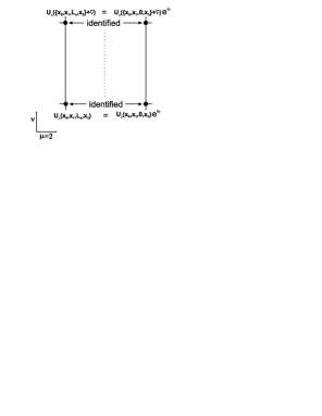
Figure 1: The plaquette presentation of the twisted boundary conditions.

The lattice variables (in the Abelian parametrization) in the presence of the magnetic flux $\varphi$ are

$$U_{\mu}(x)=\left(\begin{array}[]{cc}\cos\phi_{\mu}(x)e^{i(\theta_{\mu}(x)+\varphi_{\mu}(x))}&\sin\phi_{\mu}(x)e^{i\chi_{\mu}(x)}\\ -\sin\phi_{\mu}(x)e^{-i\chi_{\mu}(x)}&\cos\phi_{\mu}(x)e^{-i(\theta_{\mu}(x)+\varphi_{\mu}(x))}\end{array}\right),$$ (15)

where $\varphi_{\mu}(x)=\varphi$ for the edge links at $x=(x_{0},x_{1},L_{s},x_{3})$ with $\mu=2$ and $\varphi_{\mu}(x)=0$ for other links.

The total flux through the plane spanned by the plaquettes $p$, which affects the edge links at $x=(x_{0},x_{1},L_{s},x_{3})$ with $\mu=2$, is

$$g\Phi=\sum_{p\in plane}(\theta_{p}+\varphi),$$ (16)

$$\theta_{p}=\theta_{\mu\nu}(x)=\theta_{\mu}(x)+\theta_{\nu}(x+a\hat{\mu})-\theta_{\mu}(x+a\hat{\nu})-\theta_{\nu}(x).$$ (17)

Eq. (16) is the lattice analogue of the flux in the continuum:

$$\Phi_{c}=\int_{S}d^{2}\sigma_{\mu\nu}F_{\mu\nu}.$$ (18)

In this approach the variable $\varphi$ describes a flux through the whole lattice plane, not just through an elementary plaquette.

The t.b.c. for the components (15),

$$U_{\mu}^{0}(x) = \cos(\theta_{\mu}(x)+\varphi_{\mu}(x))\cos\phi_{\mu}(x),$$ (19)

$$U_{\mu}^{1}(x) = \sin\phi_{\mu}(x)\cos\chi_{\mu}(x),$$

$$U_{\mu}^{2}(x) = \sin\phi_{\mu}(x)\sin\chi_{\mu}(x),$$

$$U_{\mu}^{3}(x) = \sin(\theta_{\mu}(x)+\varphi_{\mu}(x))\cos\phi_{\mu}(x),$$

read

$$U^{0}_{\mu}(x)=\Biggl{\{}\begin{array}[]{l}U^{0}_{\mu}(x)\cos\varphi-U^{3}_{\mu}(x)\sin\varphi\leavevmode\nobreak\ \leavevmode\nobreak\ \leavevmode\nobreak\ \leavevmode\nobreak\ $for$\leavevmode\nobreak\ x=\{x_{0},x_{1},L_{s},x_{3}\}\leavevmode\nobreak\ $and$\leavevmode\nobreak\ \mu=2,\\ U^{0}_{\mu}(x)\hskip 108.12054pt\leavevmode\nobreak\ $for other links$,\end{array}$$ (22)

$$U^{3}_{\mu}(x)=\Biggl{\{}\begin{array}[]{l}U^{0}_{\mu}(x)\sin\varphi+U^{3}_{\mu}(x)\cos\varphi\leavevmode\nobreak\ \leavevmode\nobreak\ \leavevmode\nobreak\ \leavevmode\nobreak\ $for$\leavevmode\nobreak\ x=\{x_{0},x_{1},L_{s},x_{3}\}\leavevmode\nobreak\ $and$\leavevmode\nobreak\ \mu=2,\\ U^{3}_{\mu}(x)\hskip 108.12054pt\leavevmode\nobreak\ $for other links$.\end{array}$$ (25)

The relations (22) and (25) have been implemented into the kernel of the MC procedure in order to produce the configurations with the magnetic flux $\varphi$. In this case the flux $\varphi$ is accounted for in obtaining a Boltzmann ensemble at each MC iteration.

3 Description of simulations and data fits

The MC simulations are carried out by means of the heat bath method. The lattices $2\times 8^{3}$, $2\times 16^{3}$ and $4\times 8^{3}$ at $\beta=3.0$, $5.0$ are considered. These values of the coupling constant correspond to the deconfinement phase and perturbative regime. To thermalize the system, 200-500 iterations are fulfilled. At each working iteration, the plaquette value (5) is averaged over the whole lattice leading to the Wilson action (4). Then the effective action is calculated by averaging over the 1000-5000 working iterations. By setting a set of magnetic fluxes $\varphi$ in the MC simulations we obtain the corresponding set of values of the effective action. The value of the condensed magnetic flux $\varphi_{min}$ is obtained as the result of the minimization of the free energy density (3).

The spontaneous generation of magnetic field is the effect of order $\sim g^{4}$ [4]. The results of MC simulations show the comparably large dispersion. So, the large amount of the MC data is collected and the standard $\chi^{2}$-method for the analysis of data is applied to determine the effect. We consider the results of the MC simulations as observed ‘‘experimental data’’.

The effective action depends smoothly on the flux $\varphi$ in the region $\varphi\sim 0$. Therefore, the free energy density can be fitted by the quadratic function of the flux $\varphi$,

$$F(\varphi)=F_{min}+b(\varphi-\varphi_{min})^{2}.$$ (26)

This choice is motivated also by the results obtained already in continuum field theory [13] where it was determined that free energy has a global minimum at $\varphi\not=0$. The parametrization (26) is the most reasonable in this case. It is based on the effective action accounting for the one-loop plus daisy diagrams [13],

$$F(H)=\frac{H^{2}}{2}+\frac{11}{48}\frac{g^{2}}{\pi^{2}}H^{2}\log\frac{T^{2}}{\mu^{2}}-\frac{1}{3}\frac{(gH)^{3/2}T}{\pi}-\frac{1}{12}{\leavevmode\nobreak\ \rm Tr\leavevmode\nobreak\ }\left[\Pi_{00}(0)\right]^{3/2},$$ (27)

having $g^{2}$ and $(g^{2})^{3/2}$ orders in coupling constant. Here, $H$ is field strength (flux $\varphi\sim H$), $T$ is the temperature, $\mu$ is the normalization point, $\Pi_{00}(0)$ is the zero–zero component of the gluon polarazation operator calculated in the external field at the finite temperature and taken at zero momentum. The value of $\beta=3$, which was used, corresponds to a deep perturbation regime. So, a comparison with perturbation results is reasonable. The systematic errors in fitting function (26) could come from not taking into account the high-order diagrams in (27). However, as it is well known [15], the lack of an expansion parameter at finite temperature starts from the three-loop diagram contributions that is of $g^{6}$ order and could not remove an effect derived in $g^{2}$ and $g^{3}$ orders. As the finite-size effects are concerned, in the present investigation we just made calculations for two lattices $2\times 8^{3}$ and $2\times 16^{3}$ and have derived the same results for the $\varphi_{min}$ (as it will be seen below). A more detailed investigation of this issue requires much more computer resources, which were limited.

There are 3 unknown parameters, $F_{min}$, $b$ and $\varphi_{min}$ in Eq.(26). The parameter $\varphi_{min}$ denotes the minimum position of the free energy, whereas the $F_{min}$ and $b$ are the free energy density at the minimum and the curvature of the free energy function, correspondingly.

The value $\varphi_{min}$ is obtained as the result of the minimization of the $\chi^{2}$-function

$$\chi^{2}(F_{min},b,\varphi_{min})=\sum_{i}\frac{(F_{min}+b(\varphi_{i}-\varphi_{min})^{2}-F(\varphi_{i}))^{2}}{D(F(\varphi_{i}))},$$ (28)

where $\varphi_{i}$ is the array of the set fluxes and $D(F(\varphi_{i}))$ is the data dispersion. It can be obtained by collecting the data into the bins (as a function of flux),

$$D(F(\varphi_{i}))=\sum_{i\in bin}\frac{(F(\varphi_{i})-\hat{F}_{bin})^{2}}{n_{bin}-1},$$ (29)

where $n_{bin}$ is the number of points in the considered bin, $\hat{F}_{bin}$ is the mean value of free energy density in the considered bin. As it is determined in the data analysis, the dispersion is independent of the magnetic flux values $\varphi$. The deviation of $\varphi_{min}$ from zero indicates the presence of spontaneously generated field.

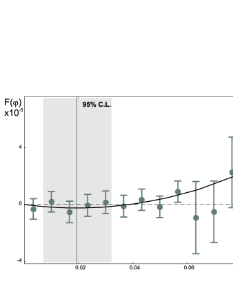
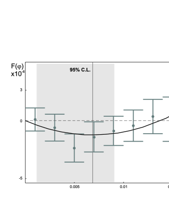
Figure 2: $\chi^{2}$-fit of the free energy density on lattice $2\times 8^{3}$ (left figure) and $2\times 16^{3}$ (right figure) for $\beta=3.0$ (grey regions describe the $\varphi_{min}=0.019^{+0.013}_{-0.012}$ and $\varphi_{min}=0.0069^{+0.0022}_{-0.0057}$, at the 95% C.L., correspondingly).

Table 1: The values of the generated fluxes $\varphi_{min}$ for different lattices (at the $95\%$ C.L.).

	$2\times 8^{3}$	$2\times 16^{3}$	$4\times 8^{3}$
$\beta=3.0$	${0.019^{+0.013}_{-0.012}}$	$0.0069^{+0.0022}_{-0.0057}$	$0.005^{+0.005}_{-0.003}$
$\beta=5.0$	${0.020^{+0.011}_{-0.010}}$

The fit results are given in the Table 1. As one can see, $\varphi_{min}$ demonstrates the $2\sigma$-deviation from zero. The dependence of $\varphi_{min}$ on the temperature is also in accordance with the results known in perturbation theory: the increase in temperature results in the increase of the field strength [4].

The fits for the lattices $2\times 8^{3}$ and $2\times 16^{3}$ at $\beta=3.0$ are shown in Fig. 2. The maximum-likelihood estimate of $F(\varphi)$ by the whole data set is shown as the solid curve. In addition, all $\varphi$ values are divided into 15 bins. The mean values and the 95% confidence intervals are presented as points for each bin. The first 9 bins contain about 600-2000 points per bin. The large number of points in the bins allow to find the free energy $F$ with the accuracy which substantively exceeds the dispersion, $\sqrt{D(F(\varphi_{i}))}\sim 10^{-4}$. It makes possible to detect the effect of interest. As it is also seen, the maximum-likelihood estimate of $F(\varphi)$ is in a good accordance with the bins pointed, because the solid line is located in the 95% confidence intervals of all bins.

The 95% C.L. area of the parameters $F_{min}$ ($b$ for the right figure) and $\varphi_{min}$ is represented in Fig. 3. The black cross marks the position of the maximum-likelihood values of $F_{min}$ ($b$ for the right figure) and $\varphi_{min}$. It can be seen that the flux is positive determined. The 95% C.L. area becomes more symmetric with the center at the $F_{min}$, $b$ and $\varphi_{min}$ when the statistics is increasing. This also confirms the results of the fitting.

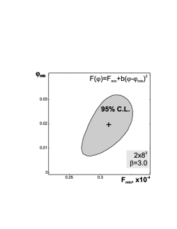
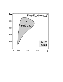
Figure 3: The 95% C.L. area for the parameters $F_{min}$ and $\varphi_{min}$, determining the free energy density dependence on the flux $\varphi_{min}$ on lattice $2\times 8^{3}$ for $\beta=3.0$ (left figure). The 95% C.L. area for the parameters $F_{min}$ and $b$ , determining the free energy density dependence on the flux $\varphi_{min}$ on lattice $2\times 16^{3}$ for $\beta=3.0$ (right figure).

4 Discussion

The main conclusion from the results obtained is that the spontaneously created temperature-dependent chromomagnetic field is present in the deconfinement phase of QCD. This supports the results derived already in the continuum quantum field theory [4, 12] and in lattice data analysis [9].

Let us first discuss the stability of the magnetic field at high temperature. It was observed in Refs. [4, 12] that the stabilization happens due to the gluon magnetic mass calculated from the one-loop polarization operator in the field at temperature. This mass has the order $m^{2}_{magn}\sim g^{2}(gH)^{1/2}T\sim g^{4}T^{2}$ as it should be because the chromomagnetic field is of order $(gH)^{1/2}\sim g^{2}T$ [4]. The stabilization is a nontrivial fact that, in principle, could be changed when the higher order Feynman diagrams to be accounted for. Now we see that the stabilization of the field really takes place.

Our approach based on the joining of calculation of the free energy functional and the consequent statistical analysis of its minimum positions at various temperatures and flux values. This overcomes the difficulties peculiar to the description of the field on a lattice. Here we mean that the field strength on a lattice is quantized and therefore a nontrivial tuning of the coupling constant, temperature and field strength values has to be done in order to determine the spontaneously created magnetic field.

We also would like to note that in the present paper the flux dependence on temperature remains not investigated in details. This is because of the small lattice size considered. That restricts the number of points permissible to study. However, at this stage we have determined the effect of interest as a whole. Even at the small lattice, one needs to take into consideration thousands points of free energy (that corresponds to an analysis of 5-10 millions MC configurations for different lattices) to determine the flux value $\varphi_{min}$ at the $95\%$ C.L. In case of larger lattices this number and corresponding computer resources should be increased considerably. This problem is left for the future.

As we mentioned in Section 2, the finite-size effects have not been investigated in detail. However, these effects are important near the phase transition temperature. They make difficult to distinguish a first-order phase transition from a second-order one. In our case, the temperature is far from $T_{c}$. The fact that external field penetrates the Coulomb phase is well known [10, 16], so the only really new thing is that this field is spontaneously created. It was first observed in continuum [4], where the field strength of order $g^{4}$ in coupling constant was established. Finite-size effects are not able to remove this result. The values $\varphi_{min}$ obtained on the lattices $2\times 8^{3}$ and $2\times 16^{3}$ (see the Table 1) are in a good agrement with each other, within the statistical errors at $95\%$ C.L.

One could speculate that the lattice sizes $2\times 8^{3}$ and $2\times 16^{3}$ are not sufficient. However, these lattice sizes were used in the Refs. [17]. The main aim of present paper is to show a possibility of spontaneous generation of chromomagnetic field at high temperature in lattice simulation, which was investigated already by perturbative methods [4, 8].

It is interesting to compare our results with that of in Ref. [10] where the response of the vacuum on the external field was investigated. These authors have observed in lattice simulations for the $SU(2)$- and $SU(3)$-gluodynamics that the external field is completely screened by the vacuum at low temperatures, as it should be in the confinement phase. With the temperature increase, the field penetrates into the vacuum and, moreover, increase in temperature results in existing more strong external fields in the vacuum. On the other hand, increase in the applied external field strength leads to the decreasing of the deconfinement temperature. These interesting properties are closely related to the studies in the present work. Actually, we have also investigated the vacuum properties as an external field problem when the field is described in terms of fluxes. This was the first step of the calculations. The next step was the statistical analysis of the minimum position of free energy, in order to determine the spontaneous creation of the field. In fact, at the first step we reproduced the results of Refs. [10] (in terms of fluxes).

Note that the present investigations also correspond to the case of the early universe. They support our previous results on the magnetic field generation in the standard model [13] and in the minimal supersymmetric standard model [14]. As it was discussed by Pollock [5], the field generated by this mechanism at the Planck era might serve as a seed field to produce the present day magnetic fields in galaxies.

We would like to conclude with the note that the deconfinement phase of gauge theories is a very interesting object to study. The temperature dependent magnetic fields, which are present in this state, influence various processes that should be taken into consideration to have an adequate concept about them.

References

- [1] D. Grasso, H. Rubinstein, Phys. Rept. 348 (2001) 163.
- [2] K. Enqvist, P. Olesen, Phys. Lett. B 329 (1994) 195.
- [3] A. Starinets, A. Vshivtsev, V. Zhukovsky, Phys. Lett. B 322 (1994) 403.
- [4] V. Skalozub, M. Bordag, Nucl. Phys. B 576 (2000) 430.
- [5] M. Pollock, Int. J. Mod. Phys. D 12 (2003) 1289.
- [6] G. Savvidy, Phys. Lett. B 71 (1977) 133.
- [7] STAR Collaboration, J. Adams, et al., Nucl. Phys. A 757 (2005) 102.
- [8] V. Skalozub, A. Strelchenko, Eur. Phys. J. C 40 (2005) 121.
- [9] N. Agasian, Phys. Lett. B 562 (2003) 257.
-
[10]
P. Cea, L. Cosmai,
Phys. Rev. D 60 (1999) 094506;
P. Cea, L. Cosmai, JHEP 0508 (2005) 079;
P. Cea, L. Cosmai, hep-lat/0101017. - [11] G. ’t Hooft, Nucl. Phys. B 153 (1979) 141.
- [12] V. Skalozub, A. Strelchenko, Eur. Phys. J. C 33 (2004) 105.
- [13] V. Demchik, V. Skalozub, Eur. Phys. J. C 25 (2002) 291.
- [14] V. Demchik, V. Skalozub, Eur. Phys. J. C 27 (2003) 601.
- [15] A. Linde, Rept. Prog. Phys. 42 (1979) 389.
- [16] M. Vettorazzo, Ph. de Forcrand, Nucl. Phys. B 686 (2004) 85.
-
[17]
T.A. DeGrand, D. Toussaint,
Phys. Rev. D 25 (1982) 526;
J. Engels, F. Karsch, H. Satz, Phys. Lett. B 101 (1981) 89;
J. Ambjorn, V. Mitrjushkin, V. Bornyakov, A. Zadorozhnyi, Phys. Lett. B 225 (1989) 153;
J. Fingberg, Urs M. Heller, V.K. Mitrjushkin, Nucl. Phys. B 435 (1995) 311.