DFTT 01/06
IFUP-TH 2006-01
DIAS-STP-06-01
High precision Monte Carlo simulations of interfaces in the three-dimensional Ising model:
a comparison with the Nambu-Goto effective string model
Michele Casellea, Martin Hasenbuschb and Marco Paneroc
a Dipartimento di Fisica Teorica dell’Università di Torino and I.N.F.N.,
Via Pietro Giuria 1, I-10125 Torino, Italy
e–mail: caselle@to.infn.it
b Dipartimento di Fisica dell’Università di Pisa and I.N.F.N.,
Largo Bruno Pontecorvo 3, I-56127 Pisa, Italy
e–mail: Martin.Hasenbusch@df.unipi.it
c School of Theoretical Physics, Dublin Institute for Advanced Studies,
10 Burlington Road, Dublin 4, Ireland
e–mail: panero@stp.dias.ie
Motivated by the recent progress in the effective string description of the interquark potential in lattice gauge theory, we study interfaces with periodic boundary conditions in the three-dimensional Ising model. Our Monte Carlo results for the associated free energy are compared with the next-to-leading order (NLO) approximation of the Nambu-Goto string model. We find clear evidence for the validity of the effective string model at the level of the NLO truncation.
1 Introduction
Recently, the effective string description of the interquark potential in lattice gauge theories (LGT) has attracted a renewed interest [1, 2, 3, 4, 5, 6, 7, 8, 9, 10, 11, 12, 13, 14, 15, 16, 17, 18]: the increased computational power and improved algorithm efficiency [19, 20, 21] have allowed to perform stringent numerical tests of the model predictions, while a better understanding of the theoretical aspects was achieved [22, 23, 24, 25, 26]. One of the plenary talks at the XXIII International Symposium on Lattice Field Theory held in Trinity College, Dublin, in July 2005 was devoted to the topic [27].
Many of the mentioned studies are focused on the behaviour of the two-point Polyakov loop correlation function: the numerical results for the free energy associated with a pair of static external sources in a pure gauge theory were compared with predictions from effective string models, as a function of the interquark distance and of the inverse temperature .
One of the simplest effective string theories is based on the action originally formulated by Nambu and Goto [28, 29]: it is a purely bosonic model, which, despite the difficulties related to anomaly and non-renormalisability, has a straightforward geometric interpretation, and for which the leading order (LO) and next-to-leading order (NLO) terms in an expansion around the classical, long-string configuration agree with the effective model proposed by Polchinski and Strominger [25]. Furthermore, the Nambu-Goto action also appears (together with other terms) in the derivation of an effective description for QCD [30, 31].
In this paper, as a further step in this direction, we compare the Nambu-Goto model with a set of high precision results on the interface free energy of the Ising spin model in three dimensions with periodic boundary conditions in the directions parallel to the interface. As it will be discussed in detail in section 2, an interface can be forced into the Ising spin system by introducing a seam of antiferromagnetic bonds through a whole cross-section of the system. Via duality, Wilson loops and Polyakov loop correlators in the gauge theory are related with interfaces in the Ising spin model: Wilson loops are mapped into interfaces with fixed boundary conditions in both directions, while Polyakov loop correlators are mapped into interfaces with periodic boundary conditions in one direction and fixed boundary conditions in the other direction. Hence, the present study is complementary to our previous work on the Polyakov-loop correlator; the periodic boundary conditions in both directions allow us to disentangle the pure string contributions from other effects, possibly (directly or indirectly) induced by fixed boundaries.
Besides these reasons of interest, which are primarily motivated by the study of confinement in lattice gauge theories, fluid interfaces are also very interesting because they have several experimental realizations, ranging from binary mixtures to amphiphilic membranes (for a review see for instance [32, 33]). Moreover the Nambu-Goto model (which is based on the assumption that the action of a given string configuration is proportional to the area of the surface spanned by the string during its time-like evolution) is closely related [33] to the so-called capillary wave model [34], which was proposed several decades ago (actually before the Nambu-Goto action), as a tool to describe interfaces in three-dimensional statistical physics systems.
Finally, it is interesting to remark that interfaces in spin models are also naturally connected to maximal ’t Hooft loops in lattice gauge theory — see, for instance, [35, 36].
The problem of the interface with periodic boundary conditions has been studied in a number of articles, particularly in the early Nineties of last century — see [37, 38] and references therein. The level of precision in these studies favoured the NLO prediction of the Nambu-Goto model against the Gaussian approximation, however it did not allow for a precise quantitative check of the NLO prediction itself.
The increase in computer power and a slightly smaller correlation length compared with [37, 38] allow us a significantly better statistical control of the next to leading order corrections considered here. In particular, our present statistics is about 1000 times larger than that of [37].
The structure of this paper is the following: in section 2 we briefly describe the introduction of an interface in the 3D Ising model, and the associated free energy; next, in section 3, we describe the numerical algorithm used in this work. Section 4 offers a review of known theoretical and numerical results, while our new results are presented in section 5. Finally, we summarise our conclusions in section 6.
2 The 3D Ising model and the interface free energy
The confined phase of the gauge model in 3D is mapped by duality into the low temperature phase of the Ising spin model, where the global symmetry is spontaneously broken and a non-vanishing magnetisation exists. According to the duality transformation, the observables of the gauge theory can be represented introducing an antiferromagnetic coupling for suitable sets of bonds in the spin model: these bonds pierce a surface having the original source lines as its boundary. This procedure can be naturally extended by introducing a seam of antiferromagnetic bonds throughout a whole time-slice on the lattice. Effectively, this amounts to imposing antiperiodic boundary conditions along the “time-like” direction, and induces an interface separating a domain of positive from a domain of negative magnetisation.111An alternative way to generate an interface in the Ising spin system would require to fix all the spin variables on the two opposite time-slices at the boundaries to the values and , respectively; however such Dirichlet boundary conditions would lead to rather large finite-size effects. Further methods to determine the interface free energy are discussed in the literature. For a collection of articles on this subject see e.g. [39].
These interfaces are the main subject of our analysis; to define the notations, we consider a periodic, cubic lattice with sizes . Let denote the coordinates of the lattice sites, with for . The action is given by:
| (1) |
Let us focus on two possible choices for the variables:
-
•
setting for all , we obtain a system with periodic boundary conditions in all directions; the corresponding partition function is denoted by ;
-
•
setting for and , and for all the remaining links we obtain a system with antiperiodic boundary conditions in the -direction and periodic boundary conditions in the remaining directions; the corresponding partition function is denoted by .
The latter choice induces an interface in the system, whose free energy222For convenience, we use the so-called “reduced free energy”, which is dimensionless. is given — in first-approximation — by the difference between the free energy of the system with anti-periodic and periodic boundary conditions: . This quantity has a characteristic -dependence, due the fact that the interface induced by the anti-periodic boundary conditions enjoys full translational invariance in the -direction. This entropy effect can be easily taken into account defining:
| (2) |
However, for large values of , an arbitrary odd (even) number of interfaces can appear in the system with antiperiodic (periodic) boundary conditions; assuming that the interfaces do not interact,333This assumption is reasonable for a low density of interfaces. the reduced interface free energy can be defined as [40]:
| (3) |
which is used in the following.
Finally, we would like to remark that the ratio of partition functions is directly related with the tunneling correlation length in a system with cylindrical geometry; for a detailed discussion see section 4.2 of [37].
3 The simulation algorithm
There are different methods available to compute the ratio of partition functions by Monte Carlo simulations.
-
•
Integration of the energy difference over , starting from a value of in the high temperature phase of the Ising spin model, where the interface tension vanishes. (See e.g. [38] and references therein.)
-
•
Snake-algorithm [21, 20]: A sequence of systems that interpolate between the periodic and anti-periodic case is defined, introducing the defects one-at-a-time; the ratio can be factored as:
(4) where is the partition function associated with the system where defects have been introduced (so that , while ). The free energy differences between and can be easily computed, as the two systems only differ by the value of on a single bond: since in general there is a sufficiently large overlap between configurations contributing to and , importance sampling with respect to the denominators on the right-hand side of eq. (4) is possible. However, for any the translational invariance in the -direction is broken. However, for sufficiently close to , the entropy gain of “depinning” becomes comparable with the energy cost and the interface starts to move along the lattice in the -direction. This causes severe autocorrelation problems in a numerical simulation of these systems.
These two choices are quite similar in spirit: the free energy difference is evaluated from the sum of many small contributions that can be easily computed. Both methods allow to investigate large interfaces, and the computational effort required for a given precision grows only with a power of the lattice size. However, the obvious practical difficulty with both methods is that a large number of individual simulations have to be run.
In the present work, we have measured the ratio of the partition functions directly, using a variant of the boundary flip algorithm [40]. As in [41], we did not actually change the boundary conditions during the simulation: rather, we counted the configurations with periodic boundary conditions that would allow for this flip. This method is efficient as long as is not too small. Since , is a rather strict upper bound on the interface size that can be reached with this method, since the signal to noise ratio decays exponentially with the interface area.444Due to our enormous statistics we could obtain a meaningful result for interface areas with slightly larger than . However, these lattice sizes are sufficient for our purpose as we shall see in the following.
For the update of the configuration, we have used the standard single cluster algorithm [42]. For most of our simulations we have used the G05CAF random number generator of the NAG library, which is a linear congruential generator characterised by , and modulus . As a check of the reliability of the random number generator, we have repeated a few of the runs for with the RANLUX generator discussed in [43], and the results are consistent with those obtained before with the G05CAF generator. Since there is no hint of a problem with the G05CAF, and the RANLUX generator is more time-consuming, we continued with the G05CAF generator.
4 Summary of results given in literature
In the following subsections we review the theoretical expectations and the numerical results which are available in the literature.
4.1 Theoretical expectations
A possible description for the dynamics of the interface in the continuum is provided by the Nambu-Goto model [28, 29]: it is based on the hypothesis that the action associated with a given interface configuration is proportional to the area of the interface itself:
| (5) |
where are the surface coordinates, while is the metric induced by the embedding in the three-dimensional space. For sake of simplicity, it is assumed that the interface can be parametrised in terms a single-valued, real function describing the transverse displacement of the surface with respect to a reference plane. This model is essentially the same as the capillary wave model [33], with the further assumption that does not depend on the direction of the normal to the infinitesimal surface element. Here we neglect the theoretical difficulties associated with the fact that the model is actually anomalous, and non-renormalisable; in the following of the discussion, the model will be regarded as an effective theory expected to describe the dynamics of the interface for sufficiently large values of (i.e. of the minimal interface area, in dimensionless units).
A perturbative expansion in powers of yields the following result for the partition function associated with the interface:
| (6) |
This expression was obtained for the first time in [44] with a zeta-function regularization and then re-obtained in [37, 45] with three other different types of regularization. In eq. (6), is a parameter that can be predicted by an argument from perturbation theory of the model in three dimensions (see below), is the modulus of the torus associated with the cross-section of the system, is Dedekind’s function:
| (7) |
and
| (8) |
where is the first Eisenstein series:
| (9) |
In most of our simulations, we have chosen ; for this choice one gets: .
In the following we shall be interested in the interface free energy, which, for square lattices of size takes the form:
| (10) |
This is the theoretical expectation which, in the following section, we shall compare with our numerical results for — see eq. (3).
4.2 Numerical results
In table 1 we have summarised numerical estimates for basic quantities at the values of studied in the present work. The result for the critical finite temperature phase transition is taken from table 4 of [49]. The interface tension is taken from table 8 of [9]. Note that in [9] only the leading order quantum corrections were used to obtain these results. The system sizes were large enough to safely ignore NLO contributions. The result for the exponential correlation length is taken from table 1 of [9]. These numbers were obtained interpolating the results of [50, 48] and from the analysis of the low temperature series [51]. The magnetisation has been computed from the interpolation formula eq. (10) of [52].
| 0.276040 | 0.65608 | 2 | 0.204864(9) | 0.644(1) | 0.85701 |
|---|---|---|---|---|---|
| 0.236025 | 0.73107 | 4 | 0.044023(3) | 1.456(3) | 0.63407 |
| 0.226102 | 0.75180 | 8 | 0.0105241(15) | 3.09(1) | 0.45311 |
5 New numerical results
In this section we present our new numerical results.
First we studied the finite effects in the interface free energy as defined by eq. (3). To this end, we run a series of simulations at with . Writing and in terms of eigenvalues of the transfer matrix (for discussion see e.g. section 4.2 of [37]), one sees that the leading corrections in to vanish as . Indeed, the results in table 2 show that the results for quickly converge with increasing . For all values of given in table 2, the choice should guarantee that corrections due to the finiteness of are far smaller than the statistical errors of our numerical estimates. In the following, we shall use also for other values of . In table 3 and in table 4 we present our results for and , respectively.
| stat/100000 | ||||
| 6 | 6 | 6 | 500 | 3.37985(29) |
| 8 | 6 | 6 | 500 | 3.38689(26) |
| 10 | 6 | 6 | 500 | 3.38989(22) |
| 12 | 6 | 6 | 500 | 3.39067(20) |
| 18 | 6 | 6 | 500 | 3.39079(17) |
| 7 | 7 | 7 | 500 | 3.97243(37) |
| 10 | 7 | 7 | 1000 | 3.99356(22) |
| 14 | 7 | 7 | 500 | 3.99783(26) |
| 21 | 7 | 7 | 599 | 3.99802(19) |
| 24 | 8 | 8 | 500 | 4.67900(28) |
| 18 | 9 | 9 | 1000 | 5.44197(35) |
| 27 | 9 | 9 | 1000 | 5.44170(28) |
| 30 | 10 | 10 | 910 | 6.29015(44) |
| 22 | 11 | 11 | 1000 | 7.22382(78) |
| 33 | 11 | 11 | 1000 | 7.22219(64) |
| 36 | 12 | 12 | 1000 | 8.2441(10) |
| 26 | 13 | 13 | 1000 | 9.3487(21) |
| 39 | 13 | 13 | 1000 | 9.3481(17) |
| 42 | 14 | 14 | 1000 | 10.5403(30) |
| 12 | 4 | 4 | 4.29672(23) |
| 15 | 5 | 5 | 6.18752(56) |
| 18 | 6 | 6 | 8.4669(16) |
| 21 | 7 | 7 | 11.1540(57) |
| 24 | 8 | 8 | 14.239(25) |
| stat/100000 | ||||
|---|---|---|---|---|
| 30 | 10 | 10 | 1000 | 3.53042(11) |
| 33 | 11 | 11 | 1000 | 3.78620(11) |
| 36 | 12 | 12 | 1000 | 4.05312(12) |
| 39 | 13 | 13 | 1000 | 4.33451(13) |
| 42 | 14 | 14 | 1000 | 4.63149(15) |
| 45 | 15 | 15 | 1000 | 4.94717(17) |
| 48 | 16 | 16 | 1000 | 5.28138(19) |
| 51 | 17 | 17 | 1000 | 5.63492(22) |
| 54 | 18 | 18 | 1000 | 6.00959(27) |
| 57 | 19 | 19 | 1000 | 6.40446(32) |
| 60 | 20 | 20 | 1000 | 6.82040(38) |
| 63 | 21 | 21 | 1000 | 7.25587(46) |
| 66 | 22 | 22 | 1326 | 7.71339(50) |
| 69 | 23 | 23 | 999 | 8.19094(72) |
| 72 | 24 | 24 | 1033 | 8.68895(88) |
| 75 | 25 | 25 | 1000 | 9.2063(12) |
| 78 | 26 | 26 | 1050 | 9.7462(14) |
| 81 | 27 | 27 | 1017 | 10.3062(19) |
| 84 | 28 | 28 | 1015 | 10.8894(25) |
| 87 | 29 | 29 | 1022 | 11.4881(33) |
| 90 | 30 | 30 | 1008 | 12.1181(45) |
5.1 Fitting the data
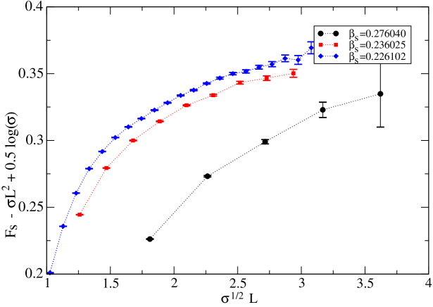
In figure 1 we have plotted as a function of the dimensionless quantity , where . The values for are taken from table 1. As , in the scaling limit, the curves for different values of should fall on top of each other. While the curve for is clearly different from the other two, those for and are close to each other — their difference being approximately constant. We have checked that these observations still hold when varying within the quoted errors. One should note that the LO effective string prediction corresponds to being constant.
Next we performed a more quantitative analysis of our data. Motivated by the theoretical prediction of eq. (6), we fitted our data with the ansatz:
| (13) |
for the interface free energy. Using the interface tension as parameter of the fit, we get results that are consistent with those in table 1. However, the statistical error of our new results for is clearly larger than the error quoted in table 1. Also, since we are mainly interested in the value of , we have fixed to the values given in table 1 in the following.
Our results for the remaining fit parameters and are shown in tables 5, 6 and 7 for , and , respectively. In these fits, we have included data for all available lattice sizes . Throughout, we have only included data obtained with .
| d.o.f. | |||
|---|---|---|---|
| 4 | 1.1500(14) | -0.430(5) | 0.81 |
| 5 | 1.154(5) | -0.45(3) | 0.92 |
| d.o.f. | |||
|---|---|---|---|
| 7 | 1.9320(5) | -0.1972(13) | 4.22 |
| 8 | 1.9348(8) | -0.208(3) | 2.37 |
| 9 | 1.9383(13) | -0.223(5) | 0.86 |
| 10 | 1.9387(22) | -0.225(11) | 1.00 |
| 11 | 1.944(4) | -0.258(22) | 0.65 |
| 12 | 1.935(7) | -0.195(48) | 0.27 |
| d.o.f. | |||
|---|---|---|---|
| 16 | 2.65513(51) | -0.1855(16) | 7.62 |
| 17 | 2.65853(65) | -0.1994(24) | 2.49 |
| 18 | 2.66067(85) | -0.2090(34) | 1.33 |
| 19 | 2.6627(11) | -0.2187(49) | 0.73 |
| 20 | 2.6636(15) | -0.2240(72) | 0.70 |
| 21 | 2.6656(20) | -0.235(10) | 0.52 |
| 22 | 2.6642(27) | -0.227(15) | 0.50 |
To estimate the effect of the error in , we redid the fits for with . This leads to slightly smaller values of , e.g. for we get . We also repeated the fit for using as input for the interface tension. This leads to a slight decrease in ; for instance, for we get instead of for ; the error on the value of that is used as input in the fits only plays a minor role.
The result at is clearly inconsistent with the prediction . However, we should note that and we should expect huge scaling corrections.
The fit results for and have similar features. In both cases, the value of increases as is increased. Also the d.o.f. decreases as is increased. For , d.o.f. is reached at , where . For the slightly larger we get: , which is fully consistent with the theoretical prediction.
For , d.o.f. is reached at , where . For we get: , which is consistent with the theoretical prediction within two units of the standard deviation.
Next we fitted our data for with the ansatz:
| (14) |
to check possible effects of higher order corrections on the numerical results for and . The results are displayed in table 8. Again, we have checked that the error of the input value for is not relevant. Now the numerical results for are smaller than the theoretical prediction . Adding higher order corrections to the fit does not allow for a more accurate numerical determination of . However these fits clearly show that the small deviation of obtained from the fit to eq. (13) can be explained by higher order corrections that are omitted in the ansatz.
| d.o.f. | ||||
|---|---|---|---|---|
| 14 | 2.6629(10) | -0.244(6) | 0.103(9) | 4.48 |
| 15 | 2.6696(14) | -0.293(9) | 0.187(15) | 1.03 |
| 16 | 2.6731(20) | -0.320(15) | 0.240(26) | 0.55 |
| 17 | 2.6713(27) | -0.305(22) | 0.207(42) | 0.52 |
| 18 | 2.6716(37) | -0.308(32) | 0.214(70) | 0.57 |
Finally, let us briefly discuss the results for . The results are quite stable for different values of . Also, fits to eq. (13) and eq. (14) give consistent results. As a final result, we quote , and for , and , respectively. Correspondingly, one gets: , and , which is somewhat larger than the theoretical prediction from [46, 38].
5.2 Results for
For we have also performed simulations for lattices with non-square cross-section (): the results of these simulations are given in table 9. In order to compare with the theoretical prediction for the NLO contribution to , we have subtracted the classical and the leading order contribution from . To this end, we have used from table 1 and from the fits summarised in table 6. For comparison, in the last column of table 9 we give the theoretical prediction for the NLO contribution — see eq. (6). The absolute value of the numerical results is found to be about larger than the theoretical prediction for the NLO contribution. This can be interpreted as an effect due to higher order corrections. It is interesting to observe that such higher order terms become more and more important as the ratio increases: this is an effect we already observed in our previous analysis of the Polyakov loop correlators [1].
| stat/100000 | LO | NLO | ||||
|---|---|---|---|---|---|---|
| 36 | 10 | 12 | 1000 | 7.1670(6) | –0.0489(6) | –0.0487 |
| 45 | 10 | 15 | 693 | 8.4449(12) | –0.0471(12) | –0.0440 |
| 54 | 10 | 18 | 1000 | 9.6976(17) | –0.0493(17) | –0.0439 |
| 60 | 10 | 20 | 1029 | 10.5235(25) | –0.0518(25) | –0.0454 |
| 66 | 10 | 22 | 999 | 11.3466(36) | –0.0521(36) | –0.0478 |
6 Conclusions
In this work, we studied interfaces in the 3D Ising model with periodic boundary conditions. We compared our numerical results for the interface free energy with predictions derived from the Nambu-Goto effective string model, which is essentially equivalent to the capillary wave model. Compared with previous work on the problem [37], the statistical errors are reduced by a factor of about 30, which allows for a quantitative check of the next-to-leading order (i.e. beyond the free string approximation) prediction. For the two coupling values closest to the phase transition, we found for a linear extension of the interface a good agreement with the next-to-leading order prediction of the Nambu-Goto model. Expressed in terms of the inverse deconfinent temperature this corresponds to . In the case of the Polyakov loop correlation function we found in [1] a similar behaviour along the compactified direction of the Polyakov loop correlator. On the contrary, along the direction with Dirichlet boundary conditions clear deviations from the Nambu-Goto string prediction were observed for distances of the order of . In fact, we actually found that the Nambu-Goto string fits the numerical data for the interquark potential at low temperatures less well than its free string approximation. Even if the presence of a boundary term in the effective string action is ruled out (at least in three dimensions) by string duality arguments [24]555Notice however that the argument of[24] only rules out the dominant boundary correction (the one which can be reinterpreted as a shift in the interquark distance [9]) but it does not exclude possible higher order boundary corrections. Notice also that the absence of such a dominant boundary corrections is compatible with the numerical data (see again [9]) on short distance Polyakov loop correlators., the above comparison between the present results and our previous analysis on the Polyakov loop correlators clearly shows that some kind of boundary correction is present in the latter case.
By virtue of the absence of boundary effects, we think that the interface free energy discussed in this paper is the perfect setting to study limits and merits of effective string models and also, if possible, to improve these effective descriptions. In this respect it would be very interesting to further analyze the deviations from the Nambu-Goto predictions which we observe in the range . Understanding the origin of these deviations remains one of the most intriguing challenges towards a consistent and satisfactory effective string description of the confining potential in lattice gauge theories.
Acknowledgements. This work was partially supported by the European Commission TMR programme HPRN-CT-2002-00325 (EUCLID). M. P. acknowledges support received from Enterprise Ireland under the Basic Research Programme. The authors would like to thank M. Billó, D. Ebert, L. Ferro and F. Maresca for useful discussions.
References
- [1] M. Caselle, M. Hasenbusch and M. Panero, JHEP 01, 076 (2006) [arXiv:hep-lat/0510107].
- [2] N. D. H. Dass and P. Majumdar, PoS LAT2005 (2005) 312 [arXiv:hep-lat/0511055].
- [3] M. Billó, M. Caselle, M. Hasenbusch and M. Panero, PoS LAT2005 (2005) 309 [arXiv:hep-lat/0511008].
- [4] M. Panero, JHEP 0505, 066 (2005) [arXiv:hep-lat/0503024].
- [5] M. Caselle, M. Hasenbusch and M. Panero, JHEP 0503, 026 (2005) [arXiv:hep-lat/0501027].
- [6] H. Meyer and M. Teper, JHEP 0412 (2004) 031 [arXiv:hep-lat/0411039].
- [7] P. Majumdar, “Continuum limit of the spectrum of the hadronic string,” arXiv:hep-lat/0406037.
- [8] M. Caselle, M. Pepe and A. Rago, JHEP 0410 (2004) 005 [arXiv:hep-lat/0406008].
- [9] M. Caselle, M. Hasenbusch and M. Panero, JHEP 0405, 032 (2004) [arXiv:hep-lat/0403004].
- [10] K. J. Juge, J. Kuti and C. Morningstar, “QCD string formation and the Casimir energy,” arXiv:hep-lat/0401032.
- [11] F. Maresca, Ph.D. thesis, Trinity College, Dublin, 2004.
- [12] Y. Koma, M. Koma and P. Majumdar, Nucl. Phys. B 692 (2004) 209 [arXiv:hep-lat/0311016].
- [13] K. J. Juge, J. Kuti, F. Maresca, C. Morningstar and M. J. Peardon, Nucl. Phys. Proc. Suppl. 129 (2004) 703 [arXiv:hep-lat/0309180].
- [14] P. Majumdar, Nucl. Phys. B 664 (2003) 213 [arXiv:hep-lat/0211038].
- [15] M. Caselle, M. Hasenbusch and M. Panero, JHEP 0301, 057 (2003) [arXiv:hep-lat/0211012].
- [16] K. J. Juge, J. Kuti and C. Morningstar, “Fine structure of the QCD string spectrum,” Phys. Rev. Lett. 90, 161601 (2003) [arXiv:hep-lat/0207004].
- [17] M. Lüscher and P. Weisz, “Quark confinement and the bosonic string,” JHEP 0207, 049 (2002) [arXiv:hep-lat/0207003].
- [18] M. Caselle, M. Panero and P. Provero, JHEP 0206, 061 (2002) [arXiv:hep-lat/0205008].
- [19] M. Lüscher and P. Weisz, JHEP 0109 (2001) 010 [arXiv:hep-lat/0108014].
- [20] M. Pepe and P. De Forcrand, Nucl. Phys. Proc. Suppl. 106 (2002) 914 [arXiv:hep-lat/0110119].
- [21] P. de Forcrand, M. D’Elia and M. Pepe, Phys. Rev. Lett. 86 (2001) 1438 [arXiv:hep-lat/0007034].
- [22] M. Billó and M. Caselle, JHEP 0507 (2005) 038 [arXiv:hep-th/0505201].
- [23] J. M. Drummond, arXiv:hep-th/0411017.
- [24] M. Lüscher and P. Weisz, JHEP 0407 (2004) 014 [arXiv:hep-th/0406205].
- [25] J. Polchinski and A. Strominger, Phys. Rev. Lett. 67 (1991) 1681.
- [26] M. Billó, M. Caselle and L. Ferro, in preparation.
- [27] J. Kuti, PoS LAT2005 (2005) 001 [arXiv:hep-lat/0511023].
- [28] T. Goto, “Relativistic Quantum Mechanics Of One-Dimensional Mechanical Continuum And Subsidiary Condition Of Dual Resonance Model,” Prog. Theor. Phys. 46, 1560 (1971).
- [29] Y. Nambu, “Strings, Monopoles, And Gauge Fields,” Phys. Rev. D 10, 4262 (1974).
- [30] Y. Koma, M. Koma, D. Ebert and H. Toki, Nucl. Phys. B 648 (2003) 189 [arXiv:hep-th/0206074].
- [31] D. Antonov, Ph.D. thesis, Humboldt-Universität zu Berlin, Berlin, 1999.
- [32] M. P. Gelfand and M. E. Fisher, Physica A 166 (1990) 1
- [33] V. Privman, Int. J. Mod. Phys. C 3 (1992) 857 [arXiv:cond-mat/9207003].
- [34] F. P. Buff, R. A. Lovett and F. H. Stillinger Jr., Phys. Rev. Lett. 15 (1965) 621
- [35] P. de Forcrand and D. Noth, Phys. Rev. D 72 (2005) 114501 [arXiv:hep-lat/0506005].
- [36] F. Bursa and M. Teper, JHEP 0508 (2005) 060 [arXiv:hep-lat/0505025].
- [37] M. Caselle, R. Fiore, F. Gliozzi, M. Hasenbusch, K. Pinn and S. Vinti, Nucl. Phys. B 432 (1994) 590 [arXiv:hep-lat/9407002].
- [38] M. Hasenbusch and K. Pinn, Physica A 245 (1997) 366, [arXiv:cond-mat/9704075].
- [39] H. J. Herrmann, W. Janke and F. Karsch (eds.), Int. J. Mod. Phys. C 3(5): Workshop on Dynamics of First Order Phase Transitions, 1-3 June 1992.
- [40] M. Hasenbusch, J.Phys. I (France) 3 (1993) 753, [arXiv:hep-lat/9209016].
- [41] M. Hasenbusch, K. Pinn and S. Vinti, arXiv:hep-lat/9806012.
- [42] U. Wolff, Phys. Rev. Lett. 62 (1989) 361.
- [43] M. Lüscher, Comput. Phys. Commun. 79 (1994) 100 [arXiv:hep-lat/9309020].
- [44] K. Dietz and T. Filk, Phys. Rev. D 27 (1983) 2944.
- [45] M. Caselle and K. Pinn, Phys. Rev. D 54 (1996) 5179 [arXiv:hep-lat/9602026].
- [46] G. Münster, Nucl. Phys. B 340 (1990) 559.
- [47] P. Provero and S. Vinti, Nucl. Phys. B 441, 562 (1995) [arXiv:hep-th/9501104].
- [48] M. Caselle and M. Hasenbusch, J. Phys. A 30, 4963 (1997) [arXiv:hep-lat/9701007].
- [49] M. Caselle and M. Hasenbusch, Nucl. Phys. B 470, 435 (1996) [arXiv:hep-lat/9511015].
- [50] V. Agostini, G. Carlino, M. Caselle and M. Hasenbusch, Nucl. Phys. B 484, 331 (1997) [arXiv:hep-lat/9607029].
- [51] H. Arisue and K. Tabata, “Low temperature series for the correlation length in d = 3 Ising model,” Nucl. Phys. B 435, 555 (1995) [arXiv:hep-lat/9407023].
- [52] A. L. Talapov and H. W. J. Blöte, J. Phys. A 29 (1996) 5727 [arXiv:cond-mat/9603013].