The CKM matrix and CP violation (in the continuum approximation)

Abstract:

The first part of this talk reviews recent developments in flavor physics that can be made without detailed understanding of hadronic physics, driven by the data. The error of $\sin 2\beta$ has shrunk below 5%, and the measurements of $\alpha$ and $\gamma$ have reached interesting precisions. For the first time, there are significant constraints on the deviations from the standard model in $B-\,\overline{\!B}$ mixing and in $b\to s$ and $b\to d$ transitions. In the second part, I review some theoretical developments for exclusive semileptonic and nonleptonic $B$ decays that have become possible using the soft-collinear effective theory. I concentrate on topics where the recent progress has model independent implications for interpreting the data. LBNL-59133, MIT-CTP 3715

PoS(LAT2005)012

1 Introduction

In the last few years the study of $CP$ violation and flavor physics has undergone dramatic developments. While for 35 years, until 1999, the only unambiguous measurement of $CP$ violation (CPV) was $\epsilon_{K}$ [1], the constraints on the Cabibbo-Kobayashi-Maskawa (CKM) matrix [2, 3] improved tremendously since the $B$ factories turned on. The error of $\sin 2\beta$ is now below 5%, and a new set of measurements started to give the best constraints on the CKM parameters.

In the standard model (SM), the masses and mixings of quarks originate from their Yukawa interactions with the Higgs condensate. We do not understand the hierarchy of the quark masses and mixing angles. Moreover, if there is new physics (NP) at the TeV scale, as suggested by the hierarchy problem, then it is not clear why it has not shown up in flavor physics experiments. A four-quark operator $(s\bar{d})^{2}/\Lambda_{\rm NP}^{2}$ with ${\cal O}(1)$ coefficient would give a contribution exceeding the measured value of $\epsilon_{K}$ unless $\Lambda_{\rm NP}\mathrel{\!\mathchoice{\lower 3.5pt\vbox{\halign{$\displaystyle\hfill#\hfil$\cr>\crcr\sim\crcr}}}{\lower 3.5pt\vbox{\halign{$\textstyle\hfill#\hfil$\cr>\crcr\sim\crcr}}}{\lower 3.5pt\vbox{\halign{$\scriptstyle\hfill#\hfil$\cr>\crcr\sim\crcr}}}{\lower 3.5pt\vbox{\halign{$\scriptscriptstyle\hfill#\hfil$\cr>\crcr\sim\crcr}}}}\!10^{4}\,{\rm TeV}$. Similarly, $(d\bar{b})^{2}/\Lambda_{\rm NP}^{2}$ yields $\Delta m_{B_{d}}$ above its measured value unless $\Lambda_{\rm NP}\mathrel{\!\mathchoice{\lower 3.5pt\vbox{\halign{$\displaystyle\hfill#\hfil$\cr>\crcr\sim\crcr}}}{\lower 3.5pt\vbox{\halign{$\textstyle\hfill#\hfil$\cr>\crcr\sim\crcr}}}{\lower 3.5pt\vbox{\halign{$\scriptstyle\hfill#\hfil$\cr>\crcr\sim\crcr}}}{\lower 3.5pt\vbox{\halign{$\scriptscriptstyle\hfill#\hfil$\cr>\crcr\sim\crcr}}}}\!10^{3}\,{\rm TeV}$. Flavor physics provides significant constraints on NP model building; for example generic SUSY models have 43 new $CP$ violating phases [4, 5], and we already know that many of them have to be suppressed not to contradict the experimental data.

Flavor and $CP$ violation were excellent probes of new physics in the past: (i) the absence of $K_{L}\to\mu^{+}\mu^{-}$ predicted the charm quark; (ii) $\epsilon_{K}$ predicted the third generation; (iii) $\Delta m_{K}$ predicted the charm mass; (iv) $\Delta m_{B}$ predicted the heavy top mass. From these measurements we knew already before the $B$ factories turned on that if there is NP at the TeV scale, it must have a very special flavor and $CP$ structure to satisfy these constraints. So what does the new data tell us?

Sections 2–4 summarize the status of $CP$ violation measurements and their implications within and beyond the SM, concentrating on measurements where the data can be interpreted without detailed understanding of the hadronic physics. Sections 5–7 deal with some recent model independent theoretical developments and their implications.

1.1 Testing the flavor sector

The only interaction that distinguishes between the fermion generations is their Yukawa couplings to the Higgs condensate. This sector of the SM contains 10 physical quark flavor parameters, the 6 quark masses and the 4 parameters in the CKM matrix: 3 mixing angles and 1 $CP$ violating phase (for reviews, see, e.g., [5, 6]). Therefore, the SM predicts intricate correlations between dozens of different decays of $s$, $c$, $b$, and $t$ quarks, and in particular between $CP$ violating observables. Possible deviations from CKM paradigm may upset some predictions:

• Subtle (or not so subtle) changes in correlations, e.g., constraints from $B$ and $K$ decays inconsistent, or $CP$ asymmetries not equal in $B\to\psi K_{S}$ and $B\to\phi K_{S}$, etc.;

• Flavor-changing neutral currents at an unexpected level, e.g., $B_{s}$ mixing incompatible with SM, enhanced $B_{(s)}\to\ell^{+}\ell^{-}$, etc.;

• Enhanced (or suppressed) $CP$ violation, e.g., in $B\to K^{*}\gamma$ or $B_{s}\to\psi\phi$.

The goal of the program is not just to determine SM parameters as precisely as possible, but to test by many overconstraining measurements whether all observable flavor-changing interactions can be explained by the SM, i.e., by integrating out virtual $W$ and $Z$ bosons and quarks. It is convenient to use the Wolfenstein parameterization of the CKM matrix,

$$V_{\rm CKM}=\pmatrix{V_{ud}&V_{us}&V_{ub}\cr V_{cd}&V_{cs}&V_{cb}\cr V_{td}&V_{ts}&V_{tb}}=\pmatrix{1-\frac{1}{2}\lambda^{2}&\lambda&A\lambda^{3}(\bar{\rho}-i\bar{\eta})\cr-\lambda&\!\!1-\frac{1}{2}\lambda^{2}\!\!&A\lambda^{2}\cr A\lambda^{3}(1-\bar{\rho}-i\bar{\eta})&-A\lambda^{2}&1}+\ldots\,,$$ (2)

which exhibits its hierarchical structure by expanding in $\lambda\simeq 0.23$, and is valid to order $\lambda^{4}$. The unitarity of the CKM matrix implies $\sum_{i}V_{ij}V_{ik}^{*}=\delta_{jk}$ and $\sum_{j}V_{ij}V_{kj}^{*}=\delta_{ik}$, and the six vanishing combinations can be represented by triangles in a complex plane. The ones obtained by taking scalar products of neighboring rows or columns are nearly degenerate, so one usually considers

$$V_{ud}\,V_{ub}^{*}+V_{cd}\,V_{cb}^{*}+V_{td}\,V_{tb}^{*}=0\,.$$ (3)

A graphical representation of this is the unitarity triangle, obtained by rescaling the best-known side to unit length (see Fig. 1). Its sides and angles can be determined in many ”redundant” ways, by measuring $CP$ violating and conserving observables. Comparing constraints on $\bar{\rho}$ and $\bar{\eta}$ provides a convenient language to compare the overconstraining measurements.

Figure 1: Sketch of the unitarity triangle.

1.2 Constraints from $K$ and $D$ decays

We knew from the measurement of $\epsilon_{K}$ that CPV in the $K$ system is at a level compatible with the SM, as $\epsilon_{K}$ can be accommodated with an ${\cal O}(1)$ value of the KM phase [3]. The other observed $CP$ violating quantity in kaon decay, $\epsilon_{K}^{\prime}$, is notoriously hard to interpret, because for the large top quark mass the electromagnetic and gluonic penguin contributions tend to cancel [10], thereby significantly amplifying the hadronic uncertainties. At present, we cannot even rule out that a large part of the measured value of $\epsilon_{K}^{\prime}$ is due to NP, and so we cannot use it to tests the KM mechanism. In the kaon sector precise tests will come from the study of $K\to\pi\nu\bar{\nu}$ decays. The $K_{L}\to\pi^{0}\nu\bar{\nu}$ decay is $CP$ violating, and therefore theoretically very clean, and there is progress in understanding the largest uncertainties in $K^{\pm}\to\pi^{\pm}\nu\bar{\nu}$ due to charm and light quark loops [11, 12]. In this mode three events have been observed so far, yielding [13]

$${\cal B}(K^{+}\to\pi^{+}\nu\bar{\nu})=\big{(}1.5^{+1.3}_{-0.9}\big{)}\times 10^{-10}\,.$$ (4)

This is consistent with the SM within the large uncertainties, but much more statistics is needed to make definitive tests.

The $D$ meson system is complementary to $K$ and $B$ mesons, because flavor and $CP$ violation are suppressed both by the GIM mechanism and by the Cabibbo angle. Therefore, CPV in $D$ decays, rare $D$ decays, and $D-\,\overline{\!D}$ mixing are predicted to be small in the SM and have not been observed. This is the only neutral meson system in which mixing generated by down-type quarks in the SM (or up-type squarks in SUSY). The strongest hint for $D^{0}-\,\overline{\!D}{}^{0}$ mixing is the lifetime difference between the $CP$-even and -odd states [14]

$$y_{CP}={\Gamma(CP\mbox{ even})-\Gamma(CP\mbox{ odd})\over\Gamma(CP\mbox{ even})+\Gamma(CP\mbox{ odd})}=(0.9\pm 0.4)\%\,.$$ (5)

Unfortunately, due to hadronic uncertainties, this central value alone could not be interpreted as a sign of new physics [15]. At the present level of sensitivity, CPV or enhanced rare decays would be the only clean signal of NP in the $D$ sector.

2 $CP$ violation in $B$ decays and the measurement of $\sin 2\beta$

2.1 $CP$ violation in decay

This is the simplest form of $CP$ violation, which can be observed in both charged and neutral meson as well as in baryon decays. If at least two amplitudes with nonzero relative weak $(\phi_{k})$ and strong $(\delta_{k})$ phases contribute to a decay,

$$A_{f}=\langle f|{\cal H}|B\rangle=\sum_{k}A_{k}\,e^{i\delta_{k}}\,e^{i\phi_{k}}\,,\qquad\overline{A}_{\overline{f}}=\langle\overline{f}|{\cal H}|\,\overline{\!B}\rangle=\sum_{k}A_{k}\,e^{i\delta_{k}}\,e^{-i\phi_{k}}\,,$$ (6)

then it is possible that $|{\overline{A}_{\overline{f}}/A_{f}}|\neq 1$, and thus $CP$ is violated.

This type of $CP$ violation is unambiguously observed in the kaon sector by $\epsilon^{\prime}_{K}\neq 0$, and now it is also established in $B$ decays [16, 17],

$$A_{K^{-}\pi^{+}}\equiv{\Gamma(\,\overline{\!B}{}^{0}\to K^{-}\pi^{+})-\Gamma(B^{0}\to K^{+}\pi^{-})\over\Gamma(\,\overline{\!B}{}^{0}\to K^{-}\pi^{+})+\Gamma(B^{0}\to K^{+}\pi^{-})}=-0.115\pm 0.018\,.$$ (7)

This is simply a counting experiment: there are $\sim 20\%$ more $B^{0}\to K^{+}\pi^{-}$ than $\,\overline{\!B}{}^{0}\to K^{-}\pi^{+}$ decays.

This measurement implies that after the ”$K$-superweak” model [18], now also ”$B$-superweak” models are excluded. I.e., models in which $CP$ violation only occurs in mixing are no longer viable. This measurement also establishes that there are sizable strong phases between the tree $(T)$ and penguin $(P)$ amplitudes in charmless $B$ decays, since $|T/P|$ is estimated to be not much larger than $|A_{K^{-}\pi^{+}}|$. Such information on strong phases will have broader implications for charmless nonleptonic decays and for understanding the $B\to K\pi$ and $\pi\pi$ rates discussed in Sec. 7.2.1.

The bottom line is that, similar to $\epsilon^{\prime}_{K}$, our theoretical understanding at present is insufficient to either prove or rule out that the $CP$ asymmetry in Eq. (7) is due to NP.

2.2 CPV in mixing

The two $B$ meson mass eigenstates are related to the flavor eigenstates via

$$|B_{L,H}\rangle=p|B^{0}\rangle\pm q|\,\overline{\!B}{}^{0}\rangle\,.$$ (8)

$CP$ is violated if the mass eigenstates are not equal to the $CP$ eigenstates. This happens if $|q/p|\neq 1$, i.e., if the physical states are not orthogonal, $\langle B_{H}|B_{L}\rangle\neq 0$, showing that this is an intrinsically quantum mechanical phenomenon.

The simplest example of this type of $CP$ violation is the semileptonic decay asymmetry to ”wrong sign” leptons. The measurements give [19]

$$A_{\rm SL}={\Gamma(\,\overline{\!B}{}^{0}(t)\to\ell^{+}X)-\Gamma(B^{0}(t)\to\ell^{-}X)\over\Gamma(\,\overline{\!B}{}^{0}(t)\to\ell^{+}X)+\Gamma(B^{0}(t)\to\ell^{-}X)}={1-|q/p|^{4}\over 1+|q/p|^{4}}=-(3.0\pm 7.8)\times 10^{-3}\,,$$ (9)

implying $|q/p|=1.0015\pm 0.0039$, where the average is dominated by a recent BELLE result [20]. In semileptonic kaon decays the similar asymmetry was measured [21], in agreement with the expectation that it is equal to $4\,{\rm Re}\,\epsilon$.

The calculation of $A_{\rm SL}$ is possible from first principles only in the $m_{b}\gg\Lambda_{\rm QCD}$ limit, using an operator product expansion to evaluate the relevant nonleptonic rates. Last year the NLO QCD calculation was completed [22, 23], predicting $A_{\rm SL}=-(5.5\pm 1.3)\times 10^{-4}$, where I averaged the central values and quoted the larger of the two theory error estimates. (The similar asymmetry in the $B_{s}$ sector is expected to be $\lambda^{2}$ smaller.) Although the experimental error in Eq. (9) is an order of magnitude larger than the SM expectation, this measurement already constraints new physics [24], as the $m_{c}^{2}/m_{b}^{2}$ suppression of $A_{\rm SL}$ in the SM can be avoided by NP.

2.3 CPV in the interference between decay with and without mixing: $B\to\psi K_{S,L}$

It is possible to obtain theoretically clean information on weak phases in $B$ decays to certain $CP$ eigenstate final states. The interference phenomena between $B^{0}\to f_{CP}$ and $B^{0}\to\,\overline{\!B}{}^{0}\to f_{CP}$ is described by

$$\lambda_{f_{CP}}=\frac{q}{p}\,\frac{\overline{A}_{f_{CP}}}{A_{f_{CP}}}=\eta_{f_{CP}}\,\frac{q}{p}\,\frac{\overline{A}_{\overline{f}_{CP}}}{A_{f_{CP}}}\,,$$ (10)

where $\eta_{f_{CP}}=\pm 1$ is the $CP$ eigenvalue of $f_{CP}$. Experimentally one can study the time dependent $CP$ asymmetry,

$$a_{f_{CP}}={\Gamma[\,\overline{\!B}{}^{0}(t)\to f]-\Gamma[B^{0}(t)\to f]\over\Gamma[\,\overline{\!B}{}^{0}(t)\to f]+\Gamma[B^{0}(t)\to f]}\qquad\\ =S_{f_{CP}}\sin(\Delta m\,t)-C_{f_{CP}}\cos(\Delta m\,t)\,,$$

where

$$S_{f}={2\,{\rm Im}\,\lambda_{f}\over 1+|\lambda_{f}|^{2}}\,,\qquad C_{f}(=-A_{f})={1-|\lambda_{f}|^{2}\over 1+|\lambda_{f}|^{2}}\,.$$ (11)

If amplitudes with one weak phase dominate a decay then $a_{f_{CP}}$ measures a phase in the Lagrangian theoretically cleanly. In this case $C_{f}=0$, and $S_{f_{CP}}={\rm Im}\,\lambda_{f_{CP}}=\sin(\arg\lambda_{f_{CP}})$, where ${\rm arg}\lambda_{f_{CP}}$ is the phase difference between the $\,\overline{\!B}{}^{0}\to f$ and $\,\overline{\!B}{}^{0}\to B^{0}\to f$ decay paths.

The theoretically cleanest example of this type of $CP$ violation is $B\to\psi K^{0}$. While there are tree and penguin contributions to the decay with different weak phases, the dominant part of the penguin amplitudes have the same weak phase as the tree amplitude. Therefore, contributions with the tree amplitude’s weak phase dominate, to an accuracy better than $\sim$1%. In the usual phase convention $S_{\psi K_{S,L}}=\mp\sin[(B\mbox{-mixing}=-2\beta)+(\mbox{decay}=0)+(K\mbox{-mixing}=0)]$, so we expect $S_{\psi K_{S,L}}=\pm\sin 2\beta$ and $C_{\psi K_{S,L}}=0$ to a similar accuracy. The current world average is

$$\sin 2\beta=0.687\pm 0.032\,,$$ (12)

which is now a 5% measurement. In the last two years the $2\beta$ vs. $\pi-2\beta$ discrete ambiguity has also been resolved by ingenious studies of the time dependent angular analysis of $B\to\psi K^{*0}$ and the time dependent Dalitz plot analysis of $B^{0}\to\,\overline{\!D}{}^{0}h^{0}$ with $\,\overline{\!D}{}^{0}\to K_{S}\pi^{+}\pi^{-}$, pioneered by BABAR [25] and BELLE [26], respectively. As a result, the negative $\cos 2\beta$ solutions are excluded, eliminating two of the four discrete ambiguities.

To summarize, $S_{\psi K}$ was the first observation of $CP$ violation outside the kaon sector, and the first observation of an ${\cal O}(1)$ $CP$ violating effect. It implies that models with approximate $CP$ symmetry (in the sense that all CPV phases are small) are excluded. The constraints on the CKM matrix from the measurements of $S_{\psi K}$, $|V_{ub}/V_{cb}|$, $\epsilon_{K}$, $B$ and $B_{s}$ mixing are shown in Fig. 2 using the CKMfitter package [27, 9]. The results throughout this paper are based on the latest averages, except for $|V_{ub}|$, for which the pre-Lepton-Photon 2005 value is used, $|V_{ub}|=(4.05\pm 0.13\pm 0.50)\times 10^{-3}$, as explained in Sec. 5.2. The overall consistency between these measurements was the first precise test of the CKM picture. It also implies that it is unlikely that ${\cal O}(1)$ deviations from the SM can occur, and one should look for corrections rather than alternatives of the CKM picture.

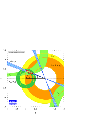
Figure 2: The present CKM fit using the measurements of $\epsilon_{K}$, $|V_{ub}/V_{cb}|$, $\Delta m_{d,s}$, and $\sin 2\beta$.

2.4 Other $CP$ asymmetries that are approximately $\sin 2\beta$ in the SM

The $b\to s$ transitions, such as $\,\overline{\!B}{}^{0}\to\phi K$, $\eta^{\prime}K$, $K^{+}K^{-}K_{S}$, etc., are dominated by one-loop (penguin) diagrams in the SM, and therefore new physics could compete with the SM contributions [28]. Using CKM unitarity we can write the contributions to such decays as a term proportional to $V_{cb}V_{cs}^{*}$ and another proportional to $V_{ub}V_{us}^{*}$. Since their ratio is about 0.02, we expect amplitudes with the $V_{cb}V_{cs}^{*}$ weak phase to dominate these decays as well. Thus, in the SM, the measurements of $-\eta_{f}S_{f}$ should agree with $S_{\psi K}$ (and $C_{f}$ should vanish) to an accuracy of order $\lambda^{2}\sim 0.05$.

If the SM and NP contributions are both significant, the $CP$ asymmetries depend on their relative size and phase, which depend on hadronic matrix elements. Since these are mode-dependent, the asymmetries will, in general, be different between the various modes, and different from $S_{\psi K}$. One may also find $C_{f}$ substantially different from 0.

Dominant $f_{CP}$ SM allowed range of${}^{\,*}$ $-\eta_{f}S_{f}$ $C_{f}$ process $|\!-\eta_{f_{CP}}S_{f_{CP}}-\sin 2\beta|$ $b\to c\bar{c}s$ $\psi K^{0}$ $<0.01$ $+0.687\pm 0.032$ $+0.016\pm 0.046$ $b\to c\bar{c}d$ $\psi\pi^{0}$ $\sim 0.2$ $+0.69\pm 0.25$ $-0.11\pm 0.20$ $D^{*+}D^{*-}$ $\sim 0.2$ $+0.67\pm 0.25$ $+0.09\pm 0.12$ $D^{+}D^{-}$ $\sim 0.2$ $+0.29\pm 0.63$ $+0.11\pm 0.36$ $b\to s\bar{q}q$ $\phi K^{0}$ $<0.05$ $+0.47\pm 0.19$ $-0.09\pm 0.14$ $\eta^{\prime}K^{0}$ $<0.05$ $+0.48\pm 0.09$ $-0.08\pm 0.07$ $\pi^{0}K_{S}$ $\sim 0.15$ $+0.31\pm 0.26$ $-0.02\pm 0.13$ $K^{+}K^{-}K_{S}$ $\sim 0.15$ $+0.51\pm 0.17$ $+0.15\pm 0.09$ $K_{S}K_{S}K_{S}$ $\sim 0.15$ $+0.61\pm 0.23$ $-0.31\pm 0.17$ $f^{0}K_{S}$ $\sim 0.25$ $+0.75\pm 0.24$ $+0.06\pm 0.21$ $\omega K_{S}$ $\sim 0.25$ $+0.63\pm 0.30$ $-0.44\pm 0.23$

Table 1: $CP$ asymmetries for which the SM predicts $-\eta_{f}S_{f}\approx\sin 2\beta$. The 3rd column contains my estimates of limits on the deviations from $\sin 2\beta$ in the SM (strict bounds are worse), and the last two columns show the world averages [19]. (The $CP$-even fractions in $K^{+}K^{-}K_{S}$ and $D^{*+}D^{*-}$ are determined experimentally.)

The averages of the latest BABAR and BELLE results are shown in Table 1. The two data sets are fairly consistent by now. The largest hint of a deviation from the SM is now in the $\eta^{\prime}K$ mode,

$$S_{\psi K}-S_{\eta^{\prime}K}=0.21\pm 0.10\,,\qquad S_{\psi K}-S_{\phi K}=0.22\pm 0.19\,,$$ (13)

which is $2\sigma$. The average $CP$ asymmetry in all $b\to s$ modes, which also equals $S_{\psi K}$ in the SM, has a bit more significant deviation, $S_{\psi K}-\langle-\eta_{f}S_{f(b\to s)}\rangle=0.18\pm 0.07$. This is currently a $2.6\sigma$ effect, however, this average is not too meaningful, because some of the modes included may deviate significantly from $S_{\psi K}$ in the SM. The third column in Table 1 shows my estimates of limits on the deviations from $S_{\psi K}$ in the SM. The hadronic matrix elements multiplying the generic ${\cal O}(0.05)$ suppression of the ”SM pollution” are hard to bound model independently [29], so strict bounds are weaker, while model calculations obtain better limits.

To understand the significance of these measurements, note that a very conservative bound using $SU(3)$ flavor symmetry using the current experimental limits on related modes gives [29, 30] $|S_{\psi K}-S_{\eta^{\prime}K}|<0.2$ in the SM. Estimates based on factorization [31] obtain deviations at the 0.02 level. Thus, $|S_{\psi K}-S_{\eta^{\prime}K}|\approx 0.2$ would be a sign of NP if established at the $5\sigma$ level. (The deviation of $S_{\phi K}$ from $S_{\psi K}$ is now statistically insignificant, but the present central value with a smaller error could still establish NP.) Such a discovery would exclude in addition to the SM, models with minimal flavor violation, and universal SUSY models, such as gauge mediated SUSY breaking.

3 Measurements of $\alpha$ and $\gamma$

To clarify terminology, I’ll call a measurement of $\gamma$ the determination of the phase difference between $b\to u$ and $b\to c$ transitions, while $\alpha(\equiv\pi-\beta-\gamma)$ will refer to the measurements of $\gamma$ in the presence of $B-\,\overline{\!B}$ mixing. The main difference between the measurements of $\gamma$ and those of the other two angles is that $\gamma$ is measured in entirely tree-level processes, so it is unlikely that new physics could modify it. It is therefore very important in searching for and constraining new physics. Interestingly, the best methods for measuring both $\alpha$ and $\gamma$ are new since 2003.

3.1 $\alpha$ from $B\to\pi\pi$, $\rho\rho$ and $\rho\pi$

In contrast to $B\to\psi K$, which is dominated by amplitudes with one weak phase, in $B\to\pi^{+}\pi^{-}$ there are two comparable contributions with different weak phases. Therefore, to determine $\alpha$ model independently, it is necessary to carry out an isospin analysis [32] (for other possibilities, see Sec. 7.2.1). The hardest ingredients are the measurement of the $\pi^{0}\pi^{0}$ rate,

$${\cal B}(B\to\pi^{0}\pi^{0})=(1.45\pm 0.29)\times 10^{-6}\,,$$ (14)

and the $CP$-asymmetry,

$${\Gamma(\,\overline{\!B}\to\pi^{0}\pi^{0})-\Gamma(B\to\pi^{0}\pi^{0})\over\Gamma(\,\overline{\!B}\to\pi^{0}\pi^{0})+\Gamma(B\to\pi^{0}\pi^{0})}=0.28\pm 0.39.$$ (15)

If these measurements were precise, one could pin down from the isospin analysis the penguin pollution, $\Delta\alpha\equiv\alpha-\alpha_{\rm eff}$ ($2\alpha_{\rm eff}={\rm arg}\,\lambda_{\pi^{+}\pi^{-}}=\arcsin[S_{\pi^{+}\pi^{-}}/(1-C_{\pi^{+}\pi^{-}}^{2})^{1/2}]$). In Fig. 3, the dark shaded region shows the confidence level using Eq. (15), while the light shaded region is the constraint without it. One finds $|\Delta\alpha|<37^{\circ}$ at 90% CL, a small improvement over the $39^{\circ}$ bound without Eq. (15). This indicates that it will take a lot more data to determine $\alpha$ precisely. In addition, the BABAR [33] and BELLE [34] results are still not quite consistent; see Table 2.

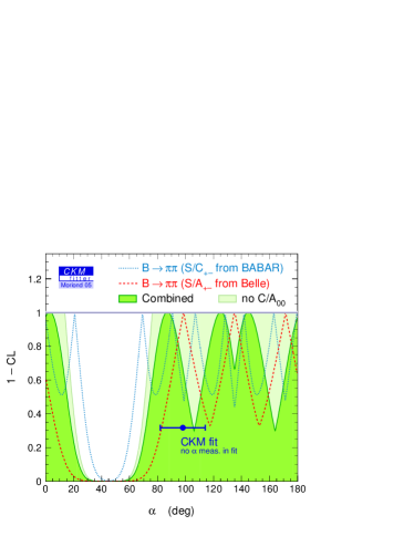
Figure 3: Constraints on $\alpha$ from $B\to\pi\pi$. Some of the eight mirror solutions may overlap.

$B\to\pi^{+}\pi^{-}$ $S_{\pi^{+}\pi^{-}}$ $C_{\pi^{+}\pi^{-}}$ BABAR $-0.30\pm 0.17$ $-0.09\pm 0.15$ BELLE $-0.67\pm 0.17$ $-0.56\pm 0.13$ average $-0.50\pm 0.12\ [0.18]$ $-0.37\pm 0.10\ [0.23]$

Table 2: $CP$ asymmetries in $B\to\pi^{+}\pi^{-}$. The brackets show the errors inflated using the PDG perscription.

The $B\to\rho\rho$ mode is more complicated than $B\to\pi\pi$, because a vector-vector ($VV$) final state is a mixture of $CP$-even ($L=0$ and 2) and -odd ($L=1$) components. The $B\to\pi\pi$ isospin analysis applies for each $L$ in $B\to\rho\rho$ (or for each transversity, and, therefore, for the longitudinal polarization component as well). The situation is simplified dramatically by the experimental observation that in the $\rho^{+}\rho^{-}$ and $\rho^{+}\rho^{0}$ modes the longitudinal polarization fraction is near unity, so the $CP$-even fraction dominates. Thus, one can simply bound $\Delta\alpha$ from [35]

$${\cal B}(B\to\rho^{0}\rho^{0})<1.1\times 10^{-6}\ (90\%\ {\rm CL})\,.$$ (16)

The smallness of this rate implies that $\Delta\alpha$ in $B\to\rho\rho$ is much smaller than in $B\to\pi\pi$. To appreciate the difference, note that ${{\cal B}(B\to\pi^{0}\pi^{0})/{\cal B}(B\to\pi^{+}\pi^{0})}=0.26\pm 0.06$, while ${\cal B}(B\to\rho^{0}\rho^{0})/{\cal B}(B\to\rho^{+}\rho^{0})<0.04\ \ (90\%\ {\rm CL})$. From $S_{\rho^{+}\rho^{-}}$ and the isospin bound on $\Delta\alpha$ one obtains

$$\alpha=96\pm 10\pm 4\pm 11^{\circ}(\alpha-\alpha_{\rm eff})\,.$$ (17)

Ultimately the isospin analysis is more complicated in $B\to\rho\rho$ than in $\pi\pi$, because the finite width of the $\rho$ allows for the final state to be in an isospin-1 state [36]. This only affects the results at the ${\cal O}(\Gamma_{\rho}^{2}/m_{\rho}^{2})$ level, which is smaller than other errors at present. With higher statistics, it will be possible to constrain this effect using the data [36].

Finally, in $B\to\rho\pi$ it is possible in principle to use a Dalitz plot analysis [37] of the interference regions of the $\pi^{+}\pi^{-}\pi^{0}$ final state to obtain a model independent determination of $\alpha$, without discrete ambiguities. The first such analysis gives [38]

$$\alpha=(113^{+27}_{-17}\pm 6)^{\circ}.$$ (18)

Viewing $B\to\rho\pi$ as two-body decays, isospin symmetry gives two pentagon relations [39]. Solving them would require measurements of the rates and $CP$ asymmetries in all the $B\to\rho^{+}\pi^{-}$, $\rho^{-}\pi^{+}$, and $\rho^{0}\pi^{0}$ modes, which are not available. BABAR and BELLE agree on the direct $CP$ asymmetries, and their average

$$A_{\pi^{-}\rho^{+}}=-0.47^{+0.13}_{-0.14}\,,\qquad A_{\pi^{+}\rho^{-}}=-0.15\pm 0.09\,,$$ (19)

is a $3.6\sigma$ signal of direct $CP$ violation, i.e., $(A_{\pi^{-}\rho^{+}}$, $A_{\pi^{+}\rho^{-}})\neq(0,0)$. Translating the available measurements to a value of $\alpha$ involves assumptions about factorization and $SU(3)$ flavor symmetry, and are theory error dominated.

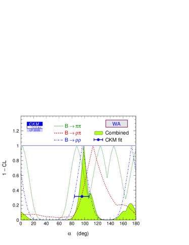
Figure 4: Confidence levels of the $\alpha$ measurements.

Combining the $\rho\rho$ and $\pi\pi$ isospin analyses with the $\rho\pi$ Dalitz plot analysis yields [9]

$$\alpha=(99^{+12}_{-9})^{\circ},$$ (20)

which is shown in Fig. 4. This direct determination of $\alpha$ is already more precise than it is from the CKM fit (without using $\alpha$ and $\gamma$), which gives $\alpha=(98\pm 16)^{\circ}$.

3.2 $\gamma$ from $B^{\pm}\to DK^{\pm}$

Here the idea is to measure the interference of $B^{-}\to D^{0}K^{-}$ ($b\to c\bar{u}s$) and $B^{-}\to\,\overline{\!D}{}^{0}K^{-}$ ($b\to u\bar{c}s$) transitions, which can be studied in final states accessible in both $D^{0}$ and $\,\overline{\!D}{}^{0}$ decays. The key is to extract the $B$ and $D$ decay amplitudes, the relative strong phases, and the weak phase $\gamma$ from the data. A practical complication is that the precision depends sensitively on the ratio of the interfering amplitudes,

$$r_{B}\equiv{A(B^{-}\to\,\overline{\!D}{}^{0}K^{-})\over A(B^{-}\to D^{0}K^{-})}\,,$$ (21)

which is around $0.1-0.2$. In the original GLW method [40, 41] one considers $D$ decays to $CP$ eigenstate final states, such as $B^{\pm}\to D^{(*)}_{CP}K^{\pm(*)}$. To overcome the smallness of $r_{B}$ and make the product of the $B$ and $D$ decay amplitudes comparable in magnitude, the ADS method [42] considers final states where Cabibbo-allowed $\,\overline{\!D}{}^{0}$ and double Cabibbo-suppressed $D^{0}$ decays interfere. So far the constraints on $\gamma$ from these analyses are fairly weak. There are other possibilities; e.g., if $r_{B}$ is not much below $\sim 0.2$ then studying single Cabibbo-suppressed $D\to KK^{*}$ decays may be advantageous [43], or in three-body $B$ decays the color suppression can be avoided [44].

It was recently realized [45, 46] that both $D^{0}$ and $\,\overline{\!D}{}^{0}$ have Cabibbo-allowed decays to certain three-body final states, such as $K_{S}\pi^{+}\pi^{-}$. This analysis can be optimized by studying the Dalitz plot dependence of the interference, and there is only a two-fold discrete ambiguity. The best present determination of $\gamma$ comes from this analysis. BELLE [47] and BABAR [48] obtained

$$\gamma=68^{+14}_{-15}\pm 13\pm 11^{\circ}\,,\qquad\gamma=67\pm 28\pm 13\pm 11^{\circ}\,,$$ (22)

where the last uncertainty is due to the $D$ decay modelling. The error is very sensitive to the central value of the amplitude ratio $r_{B}$ (and $r_{B}^{*}$ for the $D^{*}K$ channel), for which BELLE found somewhat larger central values than BABAR. The same values of $r_{B}^{(*)}$ also enter the ADS analyses, and the data can be combined to fit for $\gamma$. Combining the GLW, ADS, and Dalitz analyses, one finds [9]

$$\gamma=\big{(}63^{+15}_{-12}\big{)}^{\circ}.$$ (23)

More data will reduce the error of $\gamma$, allow for a significant measurement of $r_{B}$, and reduce the dependence on the $D$ decay modelling.

4 Implications of the $\alpha$ and $\gamma$ measurements

Since the goal of the $B$ factories is to overconstrain the CKM matrix, one should include in the CKM fit all measurements that are not limited by theoretical uncertainties. The result of such a fit is shown in the right plot in Fig. 5, which includes in addition to the inputs in Fig. 2 the above measurements of $\alpha$ and $\gamma$. The left plot shows the fit using the angle measurements only, and indicates that determination of $\bar{\rho},\bar{\eta}$ from the angles alone is almost as precise as from all inputs combined. The allowed region of $\bar{\rho},\bar{\eta}$ shrinks only slightly compared to Fig. 2, and the most interesting implication of the $\alpha$ and $\gamma$ measurements is the reduction in the allowed range of the $B_{s}-\,\overline{\!B}_{s}$ mixing frequency. While the fit in Fig. 2 gives $\Delta m_{s}=\big{(}17.9^{+10.5}_{-1.7}\,{}^{[+20.0]}_{[-2.8]}\big{)}\,{\rm ps}^{-1}$ at $1\sigma\ [2\sigma]$, the full fit gives $\Delta m_{s}=\big{(}17.9^{+3.6}_{-1.4}\,{}^{[+8.6]}_{[-2.4]}\big{)}\,{\rm ps}^{-1}$.

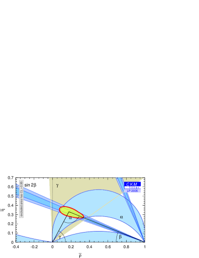
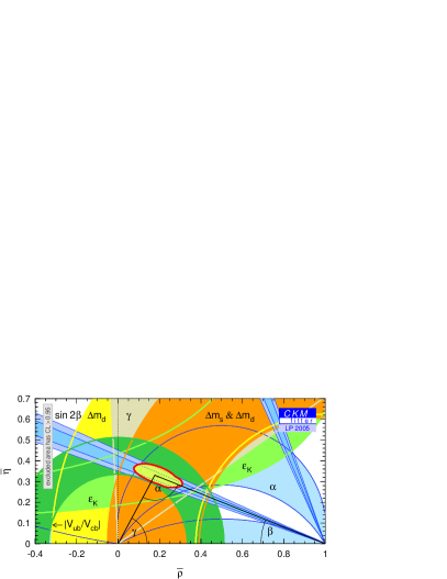
Figure 5: SM CKM fit including only the angle measurements (left), and all available measurements not limited by theoretical uncertainties (right).

4.1 New physics in $B^{0}-\,\overline{\!B}{}^{0}$ mixing

      

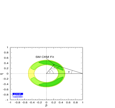
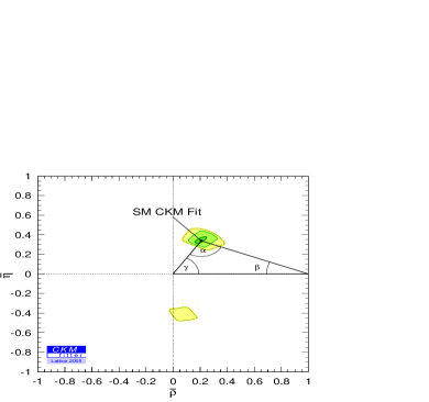
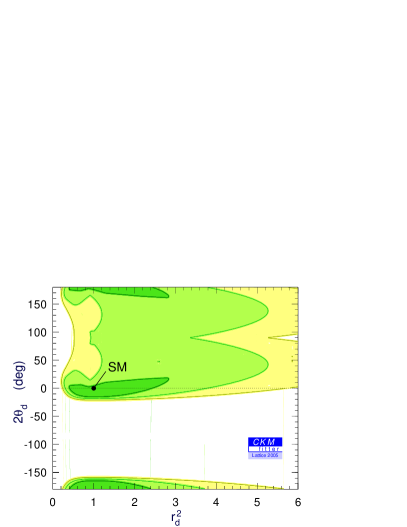
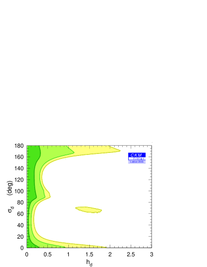
Figure 6: Allowed regions in the $\bar{\rho}-\bar{\eta}$ plane (top) and the $r_{d}^{2}-2\theta_{d}$ plane (bottom) in the presence of new physics in $B-\,\overline{\!B}$ mixing. The left [right] plots are the allowed regions without [with] the constraints on $\alpha$, $\gamma$, and $\cos 2\beta$. The dark, medium, and light shaded areas have CL $>$ 0.90, 0.32, and 0.05, respectively.

Figure 7: Allowed regions in the $h_{d}-\sigma_{d}$ plane.

In a large class of models the dominant NP effect in $B$ physics is to modify the $B^{0}-\,\overline{\!B}{}^{0}$ mixing amplitude [49], which can be parameterized as

$$M_{12}=M_{12}^{\rm(SM)}r_{d}^{2}\,e^{2i\theta_{d}}=M_{12}^{\rm(SM)}(1+h_{d}\,e^{2i\sigma_{d}}).$$ (24)

Then $\Delta m_{B}=r_{d}^{2}\,\Delta m_{B}^{\rm(SM)}$, $S_{\psi K}=\sin(2\beta+2\theta_{d})$, $S_{\rho^{+}\rho^{-}}=\sin(2\alpha-2\theta_{d})$, while the tree-level measurements $|V_{ub}/V_{cb}|$ and $\gamma$ extracted from $B\to DK$ are unaffected. Since $\theta_{d}$ drops out from $\alpha+\beta$, the measurements of $\alpha$, together with $\beta$, are effectively equivalent in these models to NP-independent measurements of $\gamma$ (up to discrete ambiguities). Measurements irrelevant for the SM CKM fit, such as the $CP$ asymmetry in semileptonic decays, $A_{\rm SL}$, become important for these constraints [24].

Figure 7 shows the fit results using only $|V_{ub}/V_{cb}|$, $\Delta m_{B}$, $S_{\psi K}$, and $A_{\rm SL}$ as inputs (left) and also including the measurements of $\alpha$, $\gamma$, and $\cos 2\beta$ (right) in the $\bar{\rho}-\bar{\eta}$ plane (top) and the $r_{d}^{2}-2\theta_{d}$ plane (bottom). The recent $\gamma$ and $\alpha$ measurements determine $\bar{\rho},\bar{\eta}$ from (effectively) tree-level $B$ decays for the first time, independent of mixing, and agree with the other SM constraints [50, 9, 51]. The disfavored ”non-SM” region around $2\theta_{d}\sim 90^{\circ}$ is due to the $\eta<0$ region in the top right plot and discrete ambiguities. Thus, NP in $B^{0}-\,\overline{\!B}{}^{0}$ mixing is severely constrained for the first time.

The $h_{d},\sigma_{d}$ parameterization is more convenient to study specific NP scenarios, since in a given model it is an additive contribution to $M_{12}^{\rm(SM)}$ that is directly calculable. The allowed range of $h_{d},\sigma_{d}$ is shown in Fig. 7. While the constraints are significant, new physics with arbitrary weak phase may still contribute to $M_{12}$ at the level of $20\%$ of the SM [52]. Similar results for the constraints on NP in $K$ and $B_{s}$ mixing can be found in Refs. [52, 53]. These constraints would not follow from just measuring each CKM element one way, and could be derived only due to overconstraining measurements.

Theoretical developments

Studying $B$ decays is not only a window to new physics, it also allows us to investigate the interplay of weak and strong interactions at a level of unprecedented detail. Many observables beyond those discussed so far are sensitive to NP, and the question is in which cases we can disentangle signals of NP from hadronic physics.

Most of the recent theoretical progress in understanding $B$ decays (using continuum methods) utilize that $m_{b}$ is much larger than $\Lambda_{\rm QCD}$. In particular, in the last few years there were significant developments toward a model independent theory of certain exclusive semileptonic and nonleptonic decays in the $m_{B}\gg\Lambda_{\rm QCD}$ limit. However, depending on the process under consideration, the relevant hadronic scale may or may not be much smaller than $m_{b}$ (and especially $m_{c}$). For example, $f_{\pi}$, $m_{\rho}$, and $m_{K}^{2}/m_{s}$ are all of order $\Lambda_{\rm QCD}$, but their numerical values span an order of magnitude. In most cases experimental guidance is needed to determine how well the theory works.

5 Inclusive semileptonic decays

5.1 $|V_{cb}|$ and $m_{b}$ from $B\to X_{c}\ell\bar{\nu}$

I would like to use the determination of $|V_{cb}|$ from inclusive semileptonic $B\to X_{c}\ell\bar{\nu}$ decay as an example to illustrate what we have learned without lattice QCD (LQCD). The state of the art is that using an operator product expansion (OPE) [54] the semileptonic rate, as well as moments of the lepton energy and the hadronic invariant mass spectra have been computed to order $\Lambda_{\rm QCD}^{3}/m_{b}^{3}$ and $\alpha_{s}^{2}\beta_{0}$. The expressions are of the form

$$\Gamma(B\to X_{c}\ell\bar{\nu})={G_{F}^{2}|V_{cb}|^{2}\over 192\pi^{3}}\,\bigg{(}{m_{\Upsilon}\over 2}\bigg{)}^{\!5}\,(0.534)$$

$$\times\!\!\! \!\!\bigg{[} \!\!\!1-0.22\Big{(}{\Lambda_{1S}\over 500\,{\rm MeV}}\Big{)}-0.011\Big{(}{\Lambda_{1S}\over 500\,{\rm MeV}}\Big{)}^{2}-0.052\Big{(}{\lambda_{1}\over(500\,{\rm MeV})^{2}}\Big{)}-0.071\Big{(}{\lambda_{2}\over(500\,{\rm MeV})^{2}}\Big{)}$$ (25)

$$- 0.006\Big{(}{\lambda_{1}\Lambda_{1S}\over(500\,{\rm MeV})^{3}}\Big{)}+0.011\Big{(}{\lambda_{2}\Lambda_{1S}\over(500\,{\rm MeV})^{3}}\Big{)}-0.006\Big{(}{\rho_{1}\over(500\,{\rm MeV})^{3}}\Big{)}+0.008\Big{(}{\rho_{2}\over(500\,{\rm MeV})^{3}}\Big{)}$$

$$+ 0.011\Big{(}{T_{1}\over(500\,{\rm MeV})^{3}}\Big{)}+0.002\Big{(}{T_{2}\over(500\,{\rm MeV})^{3}}\Big{)}-0.017\Big{(}{T_{3}\over(500\,{\rm MeV})^{3}}\Big{)}-0.008\Big{(}{T_{4}\over(500\,{\rm MeV})^{3}}\Big{)}$$

$$+ 0.096\epsilon-0.030\epsilon^{2}_{\rm BLM}+0.015\epsilon\Big{(}{\Lambda_{1S}\over 500\,{\rm MeV}}\Big{)}+\ldots\bigg{]}\,,$$

where $\Lambda_{1S}\equiv m_{\Upsilon}/2-m_{b}^{1S}$ is related to a short distance $b$ quark mass [55, 56], and the ${\cal O}(\Lambda_{\rm QCD}^{2}/m_{b}^{2})$ corrections are parameterized by $\lambda_{1,2}$. The other terms are $\Lambda_{\rm QCD}^{3}/m_{b}^{3}$ and perturbative corrections, where $\varepsilon\equiv 1$ counts the order and the BLM subscript denotes terms with the highest power of $\beta_{0}$.

Such formulae are fitted to about $90$ observables. The fits determine $|V_{cb}|$ and the hadronic parameters, and their consistency provides a powerful test of the theory. The fits have been performed in several schemes and give [57, 58],

$$|V_{cb}|=(41.7\pm 0.7)\times 10^{-3}\,,$$ (26)

where I averaged the central values and kept the error quoted in each paper. For the quark masses one gets [57, 59]

$$m_{b}^{1S}=(4.68\pm 0.03)\,{\rm GeV}\,,\qquad\overline{m}_{c}(\overline{m}_{c})=(1.22\pm 0.06)\,{\rm GeV}\,,$$ (27)

which correspond to $\overline{m}_{b}(\overline{m}_{b})=(4.18\pm 0.04)\,{\rm GeV}$ and $m_{c}^{1S}=(1.41\pm 0.05)\,{\rm GeV}$.

5.2 $B\to X_{u}\ell\bar{\nu}$, $X_{s}\gamma$ and $X_{s}\ell^{+}\ell^{-}$

One could easily spend a whole talk on inclusive heavy to light decays, but since it has little relevance for LQCD, I will be brief. The determination of $|V_{ub}|$ is more complicated than that of $|V_{cb}|$, because of the large $B\to X_{c}\ell\bar{\nu}$ background. The total $B\to X_{u}\ell\bar{\nu}$ rate is known at the 5% level [55], but the cuts used in most experimental analyses to remove the $B\to X_{c}\ell\bar{\nu}$ background introduce ${\cal O}(1)$ dependence on a nonperturbative $b$ quark light-cone distribution function (sometimes called the shape function). At leading order, one universal function occurs [60], which can be extracted from $B\to X_{s}\gamma$ and applied to the analyses of the measured $E_{\ell}$, $m_{X}$ or $P_{X}^{+}(=E_{X}-|\vec{p}_{X}|)$ spectra in $B\to X_{u}\ell\bar{\nu}$. At order $\Lambda_{\rm QCD}/m_{b}$ several new functions occur [61], and it is not known how to extract these from data. The hadronic physics being parameterized by functions is a significant complication compared to the determination of $|V_{cb}|$, where it is encoded by numbers.

A different approach is to eliminate the $B\to X_{c}\ell\bar{\nu}$ background using $q^{2}$ and $m_{X}$ cuts, in which case the local OPE remains valid [62]. The dependence on the shape function can also be reduced by extending the measurements into the $B\to X_{c}\ell\bar{\nu}$ region. Recent analyses could measure the $B\to X_{u}e\bar{\nu}$ rates for $p_{e}\geq 1.9$ GeV, which is well below the charm threshold [63].

Averaging the inclusive measurements, HFAG quotes $|V_{ub}|=(4.38\pm 0.19\pm 0.27)\times 10^{-3}$ [19], which is in slight tension with the CKM fit for $|V_{ub}|$ dominated by the $\sin 2\beta$ measurement; see Fig. 8. HFAG uses the prescription [64], and due to concerns about how the shape function model dependence and error is estimated, I use an older value of $|V_{ub}|$ (see end of Sec. 2.3).

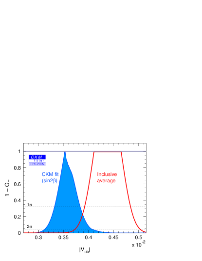
Figure 8: HFAG’s inclusive average for $|V_{ub}|$ vs. the prediction from the CKM fit.

The loop-dominated $B\to X_{s}\gamma$ and $X_{s}\ell^{+}\ell^{-}$ decays received a lot of attention, because of their sensitivity to new physics. We recently learned that both ${\cal B}(B\to X_{s}\gamma)=(3.39^{+0.30}_{-0.27})\times 10^{-4}$ and ${\cal B}(B\to X_{s}\ell^{+}\ell^{-})=(4.5\pm 1.0)\times 10^{-6}$ [19] agree with the SM at the 10% and 20% level, respectively, which is a great triumph for the SM. There is a major ongoing effort toward the NNLO calculation of ${\cal B}(B\to X_{s}\gamma)$ [65], which may reduce the perturbation theory error to $\mathrel{\!\mathchoice{\lower 3.5pt\vbox{\halign{$\displaystyle\hfill#\hfil$\cr<\crcr\sim\crcr}}}{\lower 3.5pt\vbox{\halign{$\textstyle\hfill#\hfil$\cr<\crcr\sim\crcr}}}{\lower 3.5pt\vbox{\halign{$\scriptstyle\hfill#\hfil$\cr<\crcr\sim\crcr}}}{\lower 3.5pt\vbox{\halign{$\scriptscriptstyle\hfill#\hfil$\cr<\crcr\sim\crcr}}}}\!5\%$.

As mentioned above, the $B\to X_{s}\gamma$ photon spectrum is also important for the determination of the shape function that enters many $|V_{ub}|$ measurements. It was realized recently that the same nonperturbative shape function is also relevant for $B\to X_{s}\ell^{+}\ell^{-}$ [66], where the measured rate for $q^{2}<m_{\psi}^{2}$ depends on it, because experimantally an additional cut on $m_{X_{s}}$ has to be used.

These rare decay measurements may actually make model building more interesting. The present central values of the $CP$ asymmetries, $S_{\eta^{\prime}K}$ and $S_{\phi K}$, can be reasonably accommodated by NP, such as SUSY (unlike ${\cal O}(1)$ deviations from $S_{\psi K}$ shown by the central values before 2004). While $B\to X_{s}\gamma$ mainly constrains left-right ($LR$) mass insertions in SUSY, $B\to X_{s}\ell^{+}\ell^{-}$ also constrains $RR$ and $LL$ mass insertions contributing in penguin diagrams. Thus, NP models have to satisfy a growing number of interrelated constraints.

6 Exclusive semileptonic heavy to light decays

6.1 What we knew a few years ago

I will not talk about exclusive $B\to D^{(*)}\ell\bar{\nu}$ decays. Its status using LQCD was reviewed in the next talk [67]. In $B$ decays to light mesons LQCD is also indispensible, as there is much more limited use of heavy quark symmetry (HQS) than in $B\to D^{(*)}$. Heavy quark spin symmetry implies relations between the $B\to\rho\ell\bar{\nu}$, $K^{*}\ell^{+}\ell^{-}$, and $K^{*}\gamma$ form factors in the large $q^{2}$ region [68], but it does not determine their normalization. We shall return to the small $q^{2}$ region below.

To determine $|V_{ub}|$ with sub-10% error from an exclusive decay, unquenched LQCD calculations are required, which have started to become available, so far limited to large $q^{2}$. Without using LQCD, one can combine heavy quark and chiral symmetries to form ”Grinstein-type double ratios” [69], whose deviation from unity is suppressed in both symmetry limits. For example,

$${f_{B}\over f_{B_{s}}}\times{f_{D_{s}}\over f_{D}}=1+{\cal O}\bigg{(}{m_{s}\over m_{c}}-{m_{s}\over m_{b}}\,,\;{m_{s}\over 1\,{\rm GeV}}\,{\alpha_{s}(m_{c})-\alpha_{s}(m_{b})\over\pi}\bigg{)}\,,$$ (28)

and lattice calculations indicate that the deviation from unity is indeed at the few percent level. Similar double ratios can be constructed for the semileptonic form factors [70, 71],

$${f^{(B\to\rho\ell\bar{\nu})}\over f^{(B\to K^{*}\ell^{+}\ell^{-})}}\times{f^{(D\to K^{*}\ell\bar{\nu})}\over f^{(D\to\rho\ell\bar{\nu})}}\,,$$ (29)

or for appropriately weighted $q^{2}$-spectra in these decays, and may be experimentally accessible soon. Recently, the leading power corrections to the HQS relations between the $B$ and $D$ decay form factors were analyzed [72]. With data from LHCB and a super-$B$-factory the double ratio [73]

$${{\cal B}(B\to\ell\bar{\nu})\over{\cal B}(B_{s}\to\ell^{+}\ell^{-})}\times{{\cal B}(D_{s}\to\ell\bar{\nu})\over{\cal B}(D\to\ell\bar{\nu})}$$ (30)

could give a determination of $|V_{ub}|$ with theoretical errors at the few percent level.

Interestingly, the most recent CLEO-c [74] and FOCUS [75] data are still consistent with no $SU(3)$ breaking in the $D\to\rho\ell\bar{\nu}$ vs. $D\to K^{*}\ell\bar{\nu}$ form factors. Averaging these measurements gives ${\cal B}(D^{+}\to\rho^{0}\ell^{+}\nu)/{\cal B}(D^{+}\to\,\overline{\!K}{}^{0}{}^{*}\ell^{+}\nu)=0.041\pm 0.005$, while the theoretical prediction using the measured $D\to K^{*}$ form factors and neglecting $SU(3)$ breaking in the matrix elements is 0.044 [71].

6.2 A ”one-page” introduction to SCET

To discuss recent developments in understanding the semileptonic form factors at small $q^{2}$ and some nonleptonic decays, we need to sketch some features of the soft collinear effective theory (SCET) [76, 77]. It is a theory designed to describe the interactions of energetic and low invariant mass partons in the $Q\gg\Lambda$ limit. SCET is constructed by introducing distinct fields for the relevant degrees of freedom, and a power counting parameter $\lambda$. It is convenient to distinguish two theories, SCET_I in which $\lambda=\sqrt{\Lambda_{\rm QCD}/Q}$ and SCET_II in which $\lambda=\Lambda_{\rm QCD}/Q$ [78]. They are appropriate for final states with invariant mass $Q\lambda$; i.e., SCET_I for jets and inclusive $B\to X_{s}\gamma$, $X_{u}\ell\bar{\nu}$, $X_{s}\ell^{+}\ell^{-}$ decays in the shape function regions ($m^{2}\sim\Lambda_{\rm QCD}Q$), and SCET_II for exclusive hadronic final states ($m^{2}\sim\Lambda_{\rm QCD}^{2}$). The fields in SCET are shown in Table 3. It is convenient to use light-cone coordinates, decomposing momenta as $p^{\mu}=\frac{1}{2}(\bar{n}\cdot p)n^{\mu}+p_{\perp}^{\mu}+\frac{1}{2}(n\cdot p)\bar{n}^{\mu}$, where $n^{2}=\bar{n}^{2}=0$ and $n\cdot\bar{n}=2$. For a light quark moving in the $n$ direction, $\psi(x)=\sum_{p}e^{-ip\cdot x}\big{[}\frac{1}{4}n/\bar{n}/\xi_{n,p}(x)+\frac{1}{4}\bar{n}/n/\widetilde{\xi}_{n,p}(x)\big{]}$ separates the large ($\xi_{n,p}$) and small ($\widetilde{\xi}_{n,p}$) components of the spinor, similar to HQET [79] where $b(x)=\sum_{v}e^{-im_{b}v\cdot x}\big{[}\frac{1}{2}(1+v\!\!\!\!/)h_{v}^{(b)}\!(x)+\frac{1}{2}(1-v\!\!\!\!/)\widetilde{h}_{v}^{(b)}\!(x)\big{]}$ separates the large ($h_{v}^{(b)}$) and small ($\widetilde{h}_{v}^{(b)}$) components of a $b$ quark field. Contrary to HQET, there is no superselection rule in SCET, because collinear gluons can change $p$ without any suppression.

modes fields $p=(+,-,\perp)$ $p^{2}$ collinear $\xi_{n,p},\ A_{n,q}^{\mu}$ $Q(\lambda^{2},1,\lambda)$ $Q^{2}\lambda^{2}$ soft $q_{q},\ A_{s}^{\mu}$ $Q(\lambda,\lambda,\lambda)$ $Q^{2}\lambda^{2}$ usoft $q_{us},\ A_{us}^{\mu}$ $Q(\lambda^{2},\lambda^{2},\lambda^{2})$ $Q^{2}\lambda^{4}$

Table 3: Fields and their scalings in SCET. There are no soft [ultrasoft] fields in SCET_I [SCET_II].

In matching QCD on SCET_I (and when appropriate on SCET_II) and expanding the weak currents and the Lagrangian in $\lambda$, a complication is that integrating out the off-shell degrees of freedom builds up Wilson lines. For example, the heavy to light current, $\bar{q}\,\Gamma\,b$, matches onto the SCET current $\bar{\xi}_{n,p}W\,\Gamma\,h_{v}^{(b)}$, where $W$ is a Wilson line built out of collinear gluons. The theory also requires soft and ultrasoft Wilson lines, usually denoted by $S$ and $Y$. Powerful constraints on the structure of SCET operators arise from the requirement of separate collinear, soft, and usoft gauge invariances. All fields transform under ultrasoft gauge transformation, but, for example, heavy quark fields do not transform under collinear ones. Some of the simplifications in dealing with nonperturbative phenomena in SCET_I arise from the observation that by the field redefinitions [77]

$$\xi_{n,p}=Y_{n}\,\xi_{n,p}^{(0)}\,,\qquad A_{n,q}=Y_{n}\,A_{n,q}^{(0)}\,Y_{n}^{\dagger}\,,\qquad Y_{n}={\rm P}\,\exp\Big{[}ig\int_{-\infty}^{x}{\rm d}s\,n\cdot A_{us}(ns)\Big{]}\,,$$ (31)

one can decouple at leading order in $\lambda$ the ultrasoft gluons from the collinear Lagrangian. Thus, nonperturbative usoft effects can be made explicit through factors of $Y_{n}$ in operators. This way SCET simplified the proofs of classic factorization theorems (e.g., Drell-Yan, DIS, etc. [80]) and allowed new ones to be proven to all orders in $\alpha_{s}$ (e.g., $B\to D^{+}\pi^{-}$ [81], $B\to D^{0}\pi^{0}$ [82]).

Going to subleading order in $\lambda$ is essential if one wants to study heavy to light transitions. Collinear and ultrasoft quarks cannot interact at leading order, so a particularly important term is the mixed usoft-collinear Lagrangian, ${\cal L}_{\xi q}^{(1)}$, which is suppressed by one power of $\lambda$ and allows to couple an usoft and a collinear quark to a collinear gluon [83]. We shall come back to it below.

6.3 The semileptonic form factors and $|V_{ub}|$

It has been proven using SCET that at leading order in $\Lambda_{\rm QCD}/Q$ ($Q=E,m_{b}$), to all orders in $\alpha_{s}$, the semileptonic form factors for $q^{2}\ll m_{B}^{2}$ can be written as a sum of two terms [84, 78, 85],

$$F(Q)=C_{i}(Q)\,\zeta_{i}(Q)+{m_{B}f_{B}f_{M}\over 4E^{2}}\int\!\ {\rm d}z\,{\rm d}x\,{\rm d}k_{+}\,T(z,Q)\,J(z,x,k_{+},Q)\,\phi_{M}(x)\,\phi_{B}(k_{+})\,,$$ (32)

where we omitted the $\mu$-dependences. The two terms arise from matrix elements of distinct time ordered products of the form, for example, $\int\!{\rm d}^{4}x\,T\big{[}J^{(n)}(0)\,{\cal L}_{\xi q}^{(m)}(x)\big{]}$, where $J^{(n)}$ is the expansion of the current and the ${\cal L}_{\xi q}$ terms can turn the ultrasoft spectator to a collinear quark. In Eq. (32) the second, factorizable (or hard scattering), term only contains ultrasoft fields in the combination $Y^{\dagger}h_{v}^{(b)}$ and $Y^{\dagger}q_{us}$, and is calculable in an expansion in $\alpha_{s}(\sqrt{\Lambda_{\rm QCD}m_{b}})$. The first, nonfactorizable (or form-factor), term satisfies symmetry relations [86]. For any current (Dirac structure) the nonfactorizable parts of the 3 $B\to$ pseudoscalar and the 7 $B\to$ vector meson form factors are related to just 3 universal functions in the heavy quark limit.

The two terms are of the same order in the $\Lambda_{\rm QCD}/m_{b}$ power counting. The factorizable (2nd) term contains $\alpha_{s}(\sqrt{\Lambda_{\rm QCD}m_{b}})$ explicitly, but whether the nonfactorizable (1st) term has a similar suppression at the physical value of $m_{b}$, or in the $m_{b}\to\infty$ limit when effects of order $\alpha_{s}(m_{b})$ and $\alpha_{s}(\sqrt{m_{b}\Lambda_{\rm QCD}})$ are fully accounted for is an open question. In the applications of the three often-discussed approaches, the assumptions for organizing the expansions and making predictions are

$$\mbox{SCET: 1st $\sim$ 2nd}\,,\qquad\mbox{QCDF: 2nd $\sim\alpha_{s}\times$(1st)}\,,\qquad\mbox{PQCD: 1st $\ll$ 2nd}\,.$$ (33)

In PQCD, the definition of the (non)factorizable terms also differs from the above. Clearly, what is called the leading order result and what is an $\alpha_{s}$ correction differs between these approaches. While some relations between semileptonic and nonleptonic decays can be insensitive to this, others are not. An important example is the value of $q^{2}$ where the forward-backward asymmetry in $B\to K^{*}\ell^{+}\ell^{-}$ vanishes, $A_{\rm FB}(q_{0}^{2})=0$. While $q_{0}^{2}$ is model independent when only the nonfactorizable part of the form factors are considered [87], the effect of the factorizable term is not suppressed by $\Lambda_{\rm QCD}/m_{b}$. Recent calculations show that they may in fact be sizable [88].

The determination of $|V_{ub}|$ from $B\to\pi\ell\bar{\nu}$ relies on measuring the rate and calculating the form factor $f_{+}(q^{2})$,

$${{\rm d}\Gamma(\,\overline{\!B}{}^{0}\to\pi^{+}\ell\bar{\nu})\over{\rm d}q^{2}}={G_{F}^{2}|\vec{p}_{\pi}|^{3}\over 24\pi^{3}}\,|V_{ub}|^{2}\,|f_{+}(q^{2})|^{2}\,.$$ (34)

Unquenched calculations of $f_{+}$ are only available for large $q^{2}$ (small $|\vec{p}_{\pi}|$) [89, 90], but experiment loses statistics, since the phase space is proportional to $|\vec{p}_{\pi}|^{3}$. Averaging these LQCD calculations and using data in the $q^{2}>16\,{\rm GeV}^{2}$ region yields $|V_{ub}|=(4.13\pm 0.62)\times 10^{-3}$ [19, 67].

Some of the current $|V_{ub}|$ determinations use model dependent parameterizations of $f_{+}(q^{2})$ to extend the lattice results to a larger part of the phase space, or to combine them with QCD sum rule calculations at small $q^{2}$ (which tend to give smaller values for $|V_{ub}|$ [91]). Such model dependent ingredients should be avoided; given the successes of the CKM picture, only analyses with well-defined errors are interesting. It has long been known that dispersion relations and the knowledge of $f_{+}(q^{2})$ at a few values of $q^{2}$ give strong bounds on its shape [92]. The new LQCD results revitalized this area [93, 94, 95], including the possibility of using factorization and the $B\to\pi\pi$ data to constrain $f_{+}(m_{\pi}^{2})$ [94]. Using the lattice calculations of $f_{+}$, the experimental measurements and dispersion relation to constrain $f_{+}(q^{2})$ at all $q^{2}$, yields $|V_{ub}|=(3.92\pm 0.52)\times 10^{-3}$ [96].

6.3.1 $B\to\rho\gamma$ vs. $K^{*}\gamma$

The factorization formula for the form factors in Eq. (32) also provides the basis for addressing the corrections to unity in the $SU(3)$ breaking parameters, $\xi_{\gamma}^{0,\pm}$, in the ratios

$${{\cal B}(B^{0}\to\rho^{0}\gamma)\over{\cal B}(B^{0}\to K^{*0}\gamma)}=\frac{1}{2}\,\bigg{|}{V_{td}\over V_{ts}}\bigg{|}^{2}(\xi_{\gamma}^{0})^{-2}\,,\qquad{{\cal B}(B^{\pm}\to\rho^{\pm}\gamma)\over{\cal B}(B^{\pm}\to K^{*\pm}\gamma)}=\bigg{|}{V_{td}\over V_{ts}}\bigg{|}^{2}(\xi_{\gamma}^{\pm})^{-2}\,.$$ (35)

The $\xi_{\gamma}$ are the analogs of $\xi$ that enters for $\Delta m_{B_{d}}/\Delta m_{B_{s}}$. The neutral mode gives a theoretically cleaner determination of $|V_{td}/V_{ts}|$, because the weak annihilation contribution is absent. (It is suppressed by $\Lambda_{\rm QCD}/m_{b}$, but may be numerically significant and is hard to estimate.) So far, there is no direct LQCD calculation of $\xi_{\gamma}$, and I was glad to hear at this meeting that this may soon become possible using a moving NRQCD action.

Recently, BELLE observed the exclusive $B\to(\rho/\omega)\gamma$ decay [97]. Assuming isospin symmetry, the average of the BELLE and BABAR data (without including the $\omega$) is ${\cal B}(B\to\rho\gamma)/{\cal B}(B\to K^{*}\gamma)=0.017\pm 0.006$ [19]. Using $\xi_{\gamma}=1.2\pm 0.15$ for this average [98] implies $|V_{td}/V_{ts}|=0.16\pm 0.03$. The smallness of ${\cal B}(B\to\rho\gamma)$, due to its non-observation at BABAR, may be a fluctuation or indicate that $\Delta m_{B_{s}}$ could be not near the experimental lower bound. While the theoretical error of this determination of $|V_{td}/V_{ts}|$ will not become competitive with that from $\Delta m_{B_{d}}/\Delta m_{B_{s}}$, it provides an important test of the SM, as NP could contribuite to these decays and $B-\,\overline{\!B}$ mixing differently.

6.4 Photon polarization in $B\to K^{*}\gamma$ and $X_{s}\gamma$

Although the $B\to X_{s}\gamma$ rate is correctly predicted by the SM at the 10% level, the measurement sums over the rates to left- and right-handed photons, and their ratio is also sensitive to NP. In the SM, $b$ quarks mainly decay to $s\gamma_{L}$ and $\bar{b}$ quarks to $\bar{s}\gamma_{R}$. This is easy to see at a hand-waving level, considering angular momentum conservation in the two-body $b\to s\gamma$ decay and the fact that due to the left-handed $W$ couplings the $s$ quark is left-handed in the $m_{s}\ll m_{b}$ limit. It also holds to all orders in $\alpha_{s}$ for the dominant operator $O_{7}\sim\bar{s}\,\sigma^{\mu\nu}F_{\mu\nu}(m_{b}P_{R}+m_{s}P_{L})b=\bar{s}\,(m_{b}F_{\mu\nu}^{L}+m_{s}F_{\mu\nu}^{R})b$. Here $F_{\mu\nu}^{L,R}=\frac{1}{2}(F_{\mu\nu}\pm i\widetilde{F}_{\mu\nu})$ are the field-strength tensors for $\gamma_{L,R}$, and $\widetilde{F}_{\mu\nu}=\frac{1}{2}\varepsilon_{\mu\nu\rho\lambda}F^{\rho\lambda}$.

The only observable measured so far that is sensitive to the photon polarization is the time dependent $CP$ asymmetry, which is proportional to $r=A(\,\overline{\!B}{}^{0}\to X_{f_{s}}\gamma_{R})/A(\,\overline{\!B}{}^{0}\to X_{f_{s}}\gamma_{L})$. It has been believed that $r\propto m_{s}/m_{b}$, and therefore the SM prediction for $S_{K*\gamma}$ [see Eq. (2.3)] is at the few percent level [99]. The world average is $S_{K*\gamma}=-0.13\pm 0.32$, consistent with a small value.

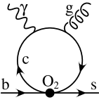
Figure 9: Dominant contribution to the ”wrong-helicity” amplitude, $A(\,\overline{\!B}{}^{0}\to X_{f_{s}}\gamma_{R})$.

It was recently realized that contributions from four-quark operators (see Fig. 9) give rise to $r$ not suppressed by $m_{s}/m_{b}$ [100]. The numerically dominant contribution is due to the matrix element of $O_{2}=(\bar{c}\,\gamma^{\mu}P_{L}b)(\bar{s}\,\gamma_{\mu}P_{L}c)$. Its contribution to the inclusive rate can be calculated reliably, and at ${\cal O}(\alpha_{s}^{2}\beta_{0})$ one finds $\Gamma(\,\overline{\!B}{}^{0}\to X_{s}\gamma_{R})/\Gamma(\,\overline{\!B}{}^{0}\to X_{s}\gamma_{L})\approx 0.01$ [100]. This suggests that for most final states, on average, $r\sim 0.1$ should be expected.

Experimentally most relevant is $r_{K^{*}}$ in the exclusive $K^{*}\gamma$ channel, which can be analyzed using SCET. (A few years ago one could have only mumbled that the contribution of Fig. 9 to $r_{K^{*}}$ is related to higher $K^{*}$ Fock states.) In the factorization formula for the form factors, Eq. (32), the second (factorizable) part contains an operator that could contribute at leading order in $\Lambda_{\rm QCD}/m_{b}$, but its $B\to K^{*}\gamma$ matrix element vanishes [100]. This proves that $r_{K^{*}}={\cal O}(\Lambda_{\rm QCD}/m_{b})$. At order $\Lambda_{\rm QCD}/m_{b}$, there are several contributions to $A(\,\overline{\!B}{}^{0}\to\,\overline{\!K}{}^{0}{}^{*}\gamma_{R})$, but there is no complete study yet. Thus, we can only estimate $A(\,\overline{\!B}{}^{0}\to\,\overline{\!K}{}^{0}{}^{*}\gamma_{R})/A(\,\overline{\!B}{}^{0}\to\,\overline{\!K}{}^{0}{}^{*}\gamma_{L})={\cal O}[(C_{2}/3C_{7})\,(\Lambda_{\rm QCD}/m_{b})]\sim 0.1$, in qualitative agreement with the inclusive calculation.

6.5 Comments on $B\to\tau\nu$

Measuring $\Delta m_{B_{s}}$ is not the only way to eliminate the error of $f_{B}$ in relating the measurement of $\Delta m_{B_{d}}$ to $|V_{td}|$. The observation of ${\cal B}(B\to\tau\nu)$ may also precede that of $\Delta m_{B_{s}}$. The $B\to\tau\nu$ measurements are usually quoted as upper bounds, but it is already interesting to look at the data. Figure 10 shows the 1 and 2$\sigma$ contours with $f_{B}=(216\pm 9\pm 21)\,$MeV [101].

If the $B\to\tau\nu$ measurement was precise, $\Gamma(B\to\tau\nu)/\Delta m_{B_{d}}$ would determine $|V_{ub}/V_{td}|$ independent of $f_{B}$ (but dependent on $B_{B_{d}}$). As shown in Fig. 10, we would get an ellipse in the $\bar{\rho},\bar{\eta}$ plane (for fixed $V_{cb}$ and $V_{ts}$). In the limit when the error of $f_{B}$ is small, the constraints are two circles that intersect at and angle $\alpha(\approx 100^{\circ})$, which is near the right angle, providing powerful constraints.

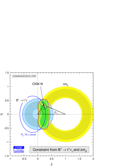
Figure 10: Constraint from $\Gamma(B\to\tau\nu)$ and $\Delta m_{B_{d}}$. Shown are the 1 and 2$\sigma$ contours.

This is another reason why pinning down $f_{B}$ is very important. While the measurement of $B\to\tau\nu$ will improve incrementally (and will be precise only at a super-$B$-factory), $\Delta m_{B_{s}}$ will almost instantly be accurate when measured. Measuring $\Delta m_{B_{s}}$ remains important not just to determine $|V_{td}/V_{ts}|$, but to constrain NP entering $B_{s}$ and $B_{d}$ mixing differently. As we have emphasized, the point is to perform overconstraining measurements and not just to determine CKM elements.

7 Nonleptonic decays

Having two hadrons in the final state is also a headache for us, using continuum methods, just like it is for you, using lattice QCD. Still, I would like to explain some recent results for two-body nonleptonic decays. This is the area where the most exciting model independent results emerged recently, and it also illustrates developments in addressing problems that will likely remain intractable with LQCD in the near future.

7.1 Factorization in $B\to D\pi$ type decays

It has long been known that in $B\to M_{1}M_{2}$ decay, if the meson $M_{1}$ that inherits the spectator quark from the $B$ is heavy and $M_{2}$ is light then ”color transparency” can justify factorization [102, 103, 104]. Traditionally, naive factorization refers to the hypothesis that one can estimate matrix elements of the four-quark operators by grouping the quark fields into a pair that can mediate $B\to M_{1}$ transition, and another pair that describes $\mbox{vacuum}\to M_{2}$ transition. We will call factorization the systematic separation of the physics associated with different momentum scales in a decay. For $\,\overline{\!B}{}^{0}\to D^{(*)+}\pi^{-}$ these notions coincide, and amount to showing that the contributions of gluons between the pion and the heavy meson are either calculable perturbatively or are suppressed by $\Lambda_{\rm QCD}/m_{b,c}$. This was proven to order $\alpha_{s}$ [104] and $\alpha_{s}^{2}$ [105], and subsequently to all orders in perturbation theory [81]. Thus, up to order $\Lambda_{\rm QCD}/Q$ and $\alpha_{s}(Q)$ corrections ($Q=E_{\pi},m_{b,c}$),

$$\langle D^{(*)}\pi|\,O_{i}(\mu_{0})|B\rangle=iN_{(*)}\,F_{B\to D^{(*)}}\,f_{\pi}\int_{0}^{1}\!{\rm d}x\;T(x,\mu_{0},\mu)\,\phi_{\pi}(x,\mu)\,.$$ (36)

The $O_{i}$ are operators in the effective Hamiltonian [106], $N_{(*)}$ is a normalization factor, $F_{B\to D^{(*)}}$ is the $B\to D^{(*)}$ form factor at $q^{2}=m_{\pi}^{2}$, $f_{\pi}$ is the pion decay constant, $T$ is a perturbatively calculable function, and $\phi(x)$ is the pion wave function.

There are three contributions to the $B\to D\pi$ amplitudes, shown in Fig. 11. SCET implies the power counting $T={\cal O}(1)$ and $C,E={\cal O}(\Lambda_{\rm QCD}/Q)$. In decays such as $\,\overline{\!B}{}^{0}\to D^{+}\pi^{-}$, which have $T$ and $C$ contributions, factorization has been observed to work at the 5–10% level. For these rates naive factorization also holds in the large $N_{c}$ limit (up to $1/N_{c}^{2}$ corrections), so detailed tests are needed to establish the mechanism responsible for factorization. At the current level of accuracy, there is no evidence for factorization becoming a worse approximation as the invariant mass of the ”light” final state increases [107], which is expected at some level if the heavy quark limit is important. The heavy quark limit also implies ${\cal B}(B^{-}\to D^{(*)0}\pi^{-})/{\cal B}(\,\overline{\!B}^{0}\to D^{(*)+}\pi^{-})=1+{\cal O}(\Lambda_{\rm QCD}/Q)$, but experimentally this ratio is around $1.8\pm 0.2$ (for all four combinations of $D,D^{*}$ and $\pi,\rho$ final states), indicating ${\cal O}(30\%)$ power corrections.

                   

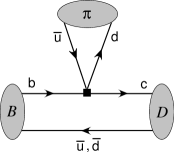
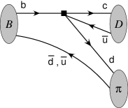
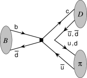
                           Tree                            Color-suppressed                       Exchange

Figure 11: Diagrams for $B$ decays, giving amplitudes $T$, $C$, and $E$. Decays to $D^{+}\pi^{-}$, $D^{0}\pi^{-}$, $D^{0}\pi^{0}$ receive $T$ and $E$, $T$ and $C$, and $C$ and $E$ contributions, respectively (from [82]).

The $B_{s}\to D_{s}\pi$ decay only proceeds via a $T$ contribution, so it can help to determine the relative size of $E$ vs. $C$. CDF measured ${\cal B}(B_{s}\to D_{s}^{-}\pi^{+})/{\cal B}(B^{0}\to D^{-}\pi^{+})\simeq 1.35\pm 0.43$ [108] (using the production ratio $f_{s}/f_{d}=0.26\pm 0.03$), the central value of which suggests that $C$ and $E$ may be comparable [109]. Since factorization relates the tree amplitudes to the semileptonic form factors, LQCD could play an important role by computing the $SU(3)$ breaking in the $B_{s}\to D_{s}\ell\bar{\nu}$ vs.  $B\to D\ell\bar{\nu}$ form factors. This is a ”gold-plated” quantity, which I hope may be found on some people’s computers in the audience.

7.1.1 Color suppressed $B\to D^{(*)0}M^{0}$ decays

The $B^{0}\to D^{0}\pi^{0}$ decay receives only $C$ and $E$ contributions, which are suppressed by $\Lambda_{\rm QCD}/Q$. These rates were beleived to be untractable until it was observed that a single class of power suppressed SCET_I operators give rise to these decays [82]. To turn the ultrasoft spectator quark in the initial $B$ into a collinear quark in the outgoing $\pi^{0}$, time ordered products with two factors of ${\cal L}_{\xi q}^{(1)}$ are needed. A factorization formula that separates the different scales was proven [82]

$$A(D^{(*)0}M^{0})=N_{0}^{M}\!\int\!\!{\rm d}z\,{\rm d}x\,{\rm d}k_{1}^{+}{\rm d}k_{2}^{+}\,T^{(i)}(z)\,J^{(i)}(z,x,k_{1}^{+},k_{2}^{+})\,S^{(i)}(k_{1}^{+},k_{2}^{+})\phi_{M}(x)+\ldots\,,$$ (37)

where $i=0,8$ label singlet and octet color structures and, for example,

$$S^{(0)}(k^{+}_{1},k^{+}_{2})=\frac{\langle D^{0}(v^{\prime})|(\bar{h}_{v^{\prime}}^{(c)}S)\,n/P_{L}(S^{\dagger}h_{v}^{(b)})(\bar{d}S)_{k^{+}_{1}}\,n/P_{L}(S^{\dagger}u)_{k^{+}_{2}}|\bar{B}^{0}(v)\rangle}{\sqrt{m_{B}m_{D}}}\,,$$ (38)

where the $S$ is a soft Wilson line in SCET_II. This is quite a different factorization than Eq. (36), as $S^{(i)}(k^{+}_{1},k^{+}_{2})$ which contain the low energy nonperturbative physics is the matrix element of a four-quark operator. It depends on the direction of the outgoing pion, $n$, and is a complex quantity, indicating that factorization can accommodate a nonperturbative strong phase.

Still, these formulae allow several nontrivial predictions to be made. The separation of scales allows one to use HQS for $S^{(i)}(k^{+}_{1},k^{+}_{2})$ without encountering $E_{\pi}/m_{c}={\cal O}(1)$ corrections, which would occur if one attempted to use HQS for this decay in full QCD. At leading order one finds the predictions $A(B\to D^{*0}M^{0})/A(B\to D^{0}M^{0})=1$ [82, 110], similar to final states with charged mesons. These are compared with the data in Fig. 12, where the ${\scriptstyle\triangle}=1$ relations follow from naive factorization and HQS, however, the $\bullet=1$ relations for the neutral modes do not, and constitute a profound prediction of SCET not foreseen by model calculations. SCET also predicted equal strong phases between the $I=1/2$ and $3/2$ amplitudes in $B\to D\pi$ and $D^{*}\pi$. The measurements, made after the prediction, give $\delta(D\pi)=(28\pm 3)^{\circ}$ and $\delta(D^{*}\pi)=(32\pm 5)^{\circ}$ [111].

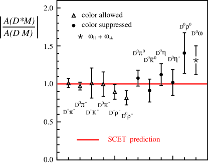
Figure 12: Ratios of the amplitudes $A(B\to D^{*0}M^{0})/A(B\to D^{0}M^{0})$ extracted from data (from [110]).

7.1.2 $\Lambda_{b}\to\Lambda_{c}\pi$ and $\Sigma_{c}^{(*)}\pi$ decays

Factorization for baryon decays does not follow from large $N_{c}$, but it still holds in the heavy quark limit at leading order in $\Lambda_{\rm QCD}/Q$, providing an interesting test. There are four contributions to $\Lambda_{b}\to\Lambda_{c}^{+}\pi^{-}$, as shown in Fig. 13, and SCET implies the power counting $T={\cal O}(1)$, $C,E={\cal O}(\Lambda_{\rm QCD}/Q)$, and $B={\cal O}(\Lambda_{\rm QCD}^{2}/Q^{2})$ [109]. The usual factorization relation connects ${\cal B}(\Lambda_{b}\to\Lambda_{c}\pi)$ measured by CDF [112] to ${\rm d}\Gamma(\Lambda_{b}\to\Lambda_{c}\ell\bar{\nu})/{\rm d}q^{2}$ at $q^{2}=m_{\pi}^{2}$ (maximal recoil). Thus, either an experimental measurement or a LQCD calculation of the $\Lambda_{b}\to\Lambda_{c}\ell\bar{\nu}$ Isgur-Wise function would allow this relation to be tested.

     

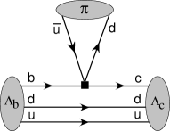
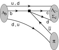
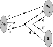
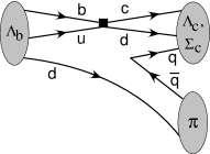
                Tree                    Color-commensurate              Exchange                        Bow tie

Figure 13: Diagrams for $\Lambda_{b}$ decays, giving amplitudes $T$, $C$, $E$, and $B$. Decay to $\Lambda_{c}$ gets contributions from all four terms. Decays to $\Sigma_{c}^{(*)}$ [$\Xi_{c}$] do not have $T$ [$T$ and $C$] contributions (from [109]).

For the power suppressed $\Lambda_{b}\to\Sigma_{c}^{(*)}\pi$ decays (we denote $\Sigma_{c}=\Sigma_{c}(2455)$ and $\Sigma_{c}^{*}=\Sigma_{c}(2520)$), naive factorization makes no sense, since the $\Lambda_{b}\to\Sigma_{c}^{(*)}$ form factors violate isospin, whereas $\Lambda_{b}\to\Sigma_{c}^{(*)}\pi$ can occur at a power suppressed level (compared to $\Lambda_{b}\to\Lambda_{c}\pi$) without isospin violation. An analysis similar to meson decays yields [109]

$${\Gamma(\Lambda_{b}\to\Sigma_{c}^{*}\pi)\over\Gamma(\Lambda_{b}\to\Sigma_{c}\pi)}={\Gamma(\Lambda_{b}\to\Sigma_{c}^{*0}\rho^{0})\over\Gamma(\Lambda_{b}\to\Sigma_{c}^{0}\rho^{0})}=2+{\cal O}\big{[}\Lambda_{\rm QCD}/Q\,,\,\alpha_{s}(Q)\big{]}\,.$$ (39)

Interestingly, this ratio is predicted to be twice as large as the similar ratios in the meson sector discussed above [82, 113, 110]. Isospin symmetry implies $\Gamma(\Lambda_{b}\to\Sigma_{c}^{(*)0}\pi^{0})=\Gamma(\Lambda_{b}\to\Sigma_{c}^{(*)+}\pi^{-})$, and similarly for the $\rho$’s. The second ratio is useful because it has no $\pi^{0}$’s in the final state, and therefore it may be easier to measure at a hadron collider (in the first ratio a $\pi^{0}$ is unavoidable either from $\Lambda_{b}\to\Sigma_{c}^{(*)0}\pi^{0}$ or from $\Lambda_{b}\to\Sigma_{c}^{(*)+}\pi^{-}\to\Lambda_{c}^{+}\pi^{0}\pi^{-}$).

7.2 Charmless $B\to M_{1}M_{2}$ decays

Factorization is more complicated for charmless $B$ decays, but I want to talk about some aspects, because these processes are in principle sensitive to new physics. In this case there is limited consensus about the implications of the heavy quark limit. In SCET a factorization formula has been proven [114, 115, 116]

$$A(B\to M_{1}M_{2})=A_{c\bar{c}} + N\Big{[}f_{M_{2}}\,\zeta^{BM_{1}}\!\int\!{\rm d}u\,T_{2\zeta}(u)\,\phi_{M_{2}}(u)$$ (40)

$${}+f_{M_{2}}\!\int\!{\rm d}z\,{\rm d}u\,T_{2J}(u,z)\,\zeta_{J}^{BM_{1}}(z)\,\phi_{M_{2}}(u)+(1\leftrightarrow 2)\Big{]}.$$

Here $\zeta_{J}^{BM_{1}}(z)=f_{M_{1}}f_{B}\int\!{\rm d}x\,{\rm d}k_{+}\,J(z,x,k_{+})\,\phi_{M_{1}}(x)\,\phi_{B}(k_{+})$ is the same object that appears in the $B\to M_{1}$ form factors in Eq. (32). Therefore, the relations to semileptonic decays do not require an expansion in $\alpha_{s}(\sqrt{\Lambda_{\rm QCD}Q})$. As we saw for the semileptonic form factors in Sec. 6.3, the nonfactorizable (1st) and factorizable (2nd) terms in square brackets are of the same order in $\Lambda_{\rm QCD}/Q$. Similar to Eq. (33), the different ways to make quantitative predictions, usually labelled SCET [114, 117, 118], QCDF [116, 119], and PQCD [120] treat the two terms differently, which has important implications for the predictions and fits to the data. The $T$’s are always calculated perturbatively. In SCET, one fits both the $\zeta$’s and $\zeta_{J}$’s; in QCDF, one fits the $\zeta$’s and calculates the $\zeta_{J}$’s perturbatively; and in PQCD the factorizable (2nd) terms dominate and depend on $k_{\perp}$.

The $A_{c\bar{c}}$ term is a possible nonperturbative contribution due to charm loops, the power counting for which is subject to debate [121]. A large $A_{c\bar{c}}$ amplitude was found in the SCET fit to $B\to\pi\pi$ [114], or adding a free parameter to the leading order QCDF result [122]. There are several model dependent calculations of this effect, referred to as ”long distance charm loops”, ”charming penguins”, and ”$D\,\overline{\!D}$ rescattering”, all of which is the same unknown physics that may yield strong phases, transverse polarization, and other ”surprises”. If one views $A_{c\bar{c}}$ as a nonperturbative term that has to be fit from data, then it can accommodate the sizable strong phase observed in $A_{K^{-}\pi^{+}}$ [see Eq. (7) where the ratio of the two interfereng amplitudes is known to be not near unity], which is hard to reproduce in QCDF (and is in the ballpark of earlier PQCD predictions). A fairly generic feature of QCDF is that it tends to predict small direct $CP$ asymmetries due to the $\alpha_{s}$ suppression of the factorizable contributions.

Another area where these effects may be important is the longitudinal polarization fraction in charmless $B$ decays to two vector mesons, such as $B\to\phi K^{*}$, $\rho\rho$, and $\rho K^{*}$. It was argued [123] that the chiral structure of the SM and the heavy quark limit imply that these decays must have longitudinal polarization fractions near unity, $1-f_{L}={\cal O}(1/m_{b}^{2})$. It is now well-established that $f_{L}(\phi K^{*})\approx 0.5$, while $f_{L}(\rho\rho)$ is near unity. Several explanations have been proposed why the data may be consistent with the SM [114, 123, 124, 125]. While $f_{L}(\phi K^{*})$ may be a result of new physics contributions (just like $A_{K^{-}\pi^{+}}$), we cannot rule out at present that it is simply due to SM physics.

7.2.1 $B\to\pi\pi$ amplitudes and $CP$ asymmetries

Since the error of $\alpha$ from the $B\to\pi\pi$ isospin analysis is large (currently $|\Delta\alpha|<37^{\circ}$, see Sec. 3.1), it will take a long time for this measurement to become precise. This makes it interesting to use more theoretical input to determine $\alpha$ without the least precisely known ingredient of the isospin analysis, the direct $CP$ asymmetry in $B\to\pi^{0}\pi^{0}$ in Eq. (15), $C_{00}$. The $\,\overline{\!B}{}^{0}$ and $B^{-}$ amplitudes to the three possible $\pi\pi$ final states are

$$\overline{A}_{+-} = -\lambda_{u}(T+P_{u})-\lambda_{c}P_{c}-\lambda_{t}P_{t}=e^{-i\gamma}\,T_{\pi\pi}-P_{\pi\pi}\,,$$

$$\sqrt{2}\,\overline{A}_{00} = \lambda_{u}(-C+P_{u})+\lambda_{c}P_{c}+\lambda_{t}P_{t}=e^{-i\gamma}\,C_{\pi\pi}+P_{\pi\pi}\,,$$

$$\sqrt{2}\,\overline{A}_{-0} = -\lambda_{u}(T+C)=e^{-i\gamma}(T_{\pi\pi}+C_{\pi\pi})\,.$$ (41)

Factorization predicts ${\rm arg}(T/C)={\cal O}(\alpha_{s},\Lambda/m_{b})$, which could eliminate the need for $C_{00}$ [117]. Due to the unknown size of $A_{c\bar{c}}$, however, the implications for the physically observable amplitudes $T_{\pi\pi}$ and $C_{\pi\pi}$ are less clear, because they are combinations of trees and penguins.

In SCET, $P_{c}$ is treated as ${\cal O}(1)$, and therefore the $P_{t}$ term is eliminated using $\lambda_{u}+\lambda_{c}+\lambda_{t}=0$. Then the $P_{\pi\pi}$ term has no weak phase, as shown in Eq. (7.2.1). In QCDF, $P_{t}$ is observed to contain ”chirally enhanced” corrections (a misnomer for terms proportional to $m_{\pi}^{2}/(m_{u}m_{b})\sim\Lambda_{\rm QCD}/m_{b}$) while $P_{c}$ is argued to be small, and therefore the $P_{c}$ term is eliminated using unitarity. Then what is meant by $T_{\pi\pi}$ and $P_{\pi\pi}$ changes, and the $P_{\pi\pi}$ term has a weak phase $e^{i\beta}$. Both approaches agree that $P_{u}$ is calculable and small.

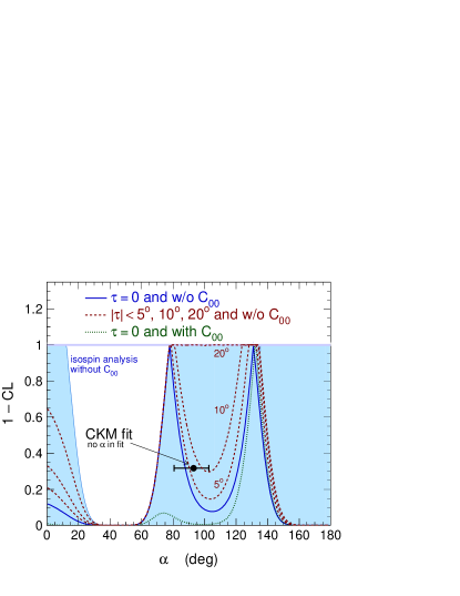
Figure 14: CL of $\alpha$ imposing $\tau=0$ with (solid) and without (dotted) the $C_{00}$ data. The constraints imposing $|\tau|<5^{\circ},10^{\circ},20^{\circ}$ are also shown (from [126]). The shaded region is the same as the green region in Fig. 3.

The central values of the $B\to\pi\pi$ data suggest significant corrections to the terms included in either approaches [126, 127]. Factorization predicts that the strong phase between the ”tree” amplitudes in $\pi^{+}\pi^{-}$ and $\pi^{-}\pi^{0}$ is small, $\tau\equiv{\rm arg}[T_{\pi\pi}/(C_{\pi\pi}+T_{\pi\pi})]={\cal O}(\alpha_{s},\Lambda/m_{b})$. As shown in Fig. 14, imposing $\tau=0$, the present data yields $\alpha\approx 78^{\circ}$ (without using $C_{00}$), somewhat below the measurement in Eq. (20). Conversely, one can ask what the SM CKM fit implies for $\tau$. The result is $\tau\sim 30^{\circ}$ [126], both in the convention of Eq. (7.2.1) and the one used in QCDF. There are several possibile resolutions: (i) $2\sigma$ level fluctuations in the data; (ii) large power corrections to $T$ or / and $C$;(iii) large up penguins; (iv) large weak annihilation; (v) or maybe something beyond the SM. It will be fascinating to find out which of these is the right explanation.

In QCDF it is problematic to accommodate the large $B\to\pi^{0}\pi^{0}$ rate in Eq. (14) [116]. This by itself is not an issue in SCET, since the factorizable ($\zeta_{J}$) term in Eq. (40) that also determines the $B\to\pi^{0}\pi^{0}$ rate is fitted from the data [114]. Color suppression is ineffective because $1/N_{c}$ is multiplied by the inverse moment of the $\pi$ distribution amplitude, $\langle\bar{u}^{-1}\rangle_{\pi}=\int_{0}^{1}{\rm d}u\,\phi_{\pi}(u)/(1-u)$, which is around 3. The $\zeta_{J}$ terms also depend on the similar inverse moment of the $B$ light-cone distribution amplitude, $\langle k_{+}^{-1}\rangle_{B}=\int\!{\rm d}k_{+}\,\phi_{B}(k_{+})/k_{+}$, and the SCET fit favors $\langle k_{+}^{-1}\rangle_{B}\sim 1/(100\,{\rm MeV})$ [128] significantly above most QCD sum rule calculations, which give $\sim\!1/(450\,{\rm MeV})$ [129].

While in $B\to\pi\pi$ the complications are due to the interference of comparable $b\to u$ tree and $b\to d$ penguin processes, $B\to K\pi$ decays are sensitive to the interference of $b\to u$ tree and the dominant $b\to s$ penguin contributions. The challenge is if one can make sufficiently precise SM predictions to be sensitive to NP. Besides the precise measurement of $A_{K^{-}\pi^{+}}$ in Eq. (7), another interesting feature of the data is the almost $4\sigma$ difference, $A_{K^{-}\pi^{0}}-A_{K^{-}\pi^{+}}=0.15\pm 0.04$. This appears to be at odds with factorization (unless subleading terms are very important, in which case the $\Lambda_{\rm QCD}/m_{b}$ expansion itself becomes questionable), because the strong phase between the penguin and the color-allowed tree amplitude is predicted to be the same as the phase between the penguin and the color-suppressed tree (up to $\Lambda_{\rm QCD}/Q$ corrections). A possible resolution is a large enhancement of electroweak penguins, or NP with the same flavor structure [130].

These are fascinating developments, however, more work and data are needed to understand why some predictions work better than $10\%$, while others receive ${\cal O}(30\%)$ corrections. Hopefully, the role of charming penguins, chirally enhanced terms, annihilation contributions, etc., can be clarified soon. We now have the tools to try to address these questions.

8 Outlook and Conclusions

The $B$ factories have provided a spectacular confirmation of the CKM picture. More interesting than the actual determinations of CKM elements is that overconstraining measurements tested the CKM picture, and we can even bound flavor models with more parameters than the SM. In particular, the comparison between tree- and loop-level measurements severely constrain NP in $B-\,\overline{\!B}$ mixing. For this, the lattice results on the decay constants and bag parameters are crucial; without it we would not yet be able to really constrain these models. This illustrates again that the program as a whole is a lot more interesting than any single measurement, since it is the multitude of overconstraining measurements and their correlations that carries the most interesting information.

Having seen these impressive measurements, one may ask where we go from here in flavor physics? Whether we see signals of flavor physics beyond the SM will be decisive. The existing measurements could have shown deviations from the SM, and if there are new particles at the TeV scale, new flavor physics could show up ”any time”. If NP is seen in flavor physics then we will want to study it in as many different processes as possible. If NP is not seen in flavor physics, then it is interesting to achieve what is theoretically possible, thereby testing the SM at a much more precise level. Even in the latter case, flavor physics will give powerful constraints on model building in the LHC era, once the masses of some new particles are known.

The present status of some of the cleanest measurements and my estimates of the theoretical limitations (using continuum methods) are summarized in Table 4. The sensitivity to NP will not be limited by hadronic physics in many measurements for a long time to come.

Measurement (in SM) Theoretical limit Present error $B\to\psi K$  ($\beta$) $\sim 0.2^{\circ}$ $1.3^{\circ}$ $B\to\eta^{\prime}K,\ \phi K,$ ($\beta$) $\sim 2^{\circ}$ $5,\ 10^{\circ}$ $B\to\rho\rho,\ \pi\pi,\ \rho\pi$  ($\alpha$) $\sim 1^{\circ}$ $\sim 13^{\circ}$ $B\to DK$  ($\gamma$) $\ll 1^{\circ}$ $\sim 20^{\circ}$ $B_{s}\to\psi\phi$  ($\beta_{s}$) $\sim 0.2^{\circ}$ — $B_{s}\to D_{s}K$  ($\gamma-2\beta_{s}$) $\ll 1^{\circ}$ — $|V_{cb}|$ $\sim 1\%$ $\sim 2\%$ $|V_{ub}|$ $\sim 5\%$ $\sim 10\%$ $B\to X_{s}\gamma$ $\sim 5\%$ $\sim 10\%$ $B\to X_{s}\ell^{+}\ell^{-}$ $\sim 5\%$ $\sim 20\%$ $B\to X_{s}\nu\bar{\nu},K^{(*)}\nu\bar{\nu}$ $\sim 5\%$ — $K^{+}\to\pi^{+}\nu\bar{\nu}$ $\sim 5\%$ $\sim 70\%$ $K_{L}\to\pi^{0}\nu\bar{\nu}$ $<1\%$ —

Table 4: Some interesting measurement that are far from being theory limited. The errors for the $CP$ asymmetries in the first box refer to the angles in parenthesis, assuming typical values for other parameters.

8.1 Where can lattice contribute the most?

• Reducing the error of the decay constants and bag parameters remains very important.

• The determinations of semileptonic form factors is in the hands of LQCD. Besides those directly relevant for the extraction of CKM elements, the computations of several others would also have important implications: we saw examples for $B_{s}\to D_{s}\ell\bar{\nu}$, $\Lambda_{b}\to\Lambda_{c}\ell\bar{\nu}$, etc.

• In addition to the $B,D\to\pi,K$ form factors, try to include the $\rho$ and $K^{*}$ final states (I know, the widths…), and attempt direct calculations at larger recoil (maybe with moving NRQCD).

• Dedicated and precise calculations of $SU(3)$ breaking in form factors and in distribution functions could also play very important roles.

• The light cone distribution functions of heavy and light mesons are important for understanding nonleptonic decays, and so far most calculations use QCD sum rules and other models.

• More remote but worthwhile goals include the calculations of nonlocal matrix elements, such as the inverse moment of the $B$ light-cone distribution amplitude, $\langle k_{+}^{-1}\rangle_{B}=\int\!{\rm d}k_{+}\,\phi_{B}(k_{+})/k_{+}$, discussed above. Not to mention nonleptonic decays…

8.2 Past and near future lessons

The large number of impressive new results speak for themselves, so it is easy to summarize the main lessons we have learned:

• $\sin 2\beta=0.687\pm 0.032$ implies that the $B$ and $K$ constraints are consistent, and the KM phase is the dominant source of CPV in flavor-changing processes.

• $S_{\psi K}-S_{\eta^{\prime}K}=0.21\pm 0.10$ and $S_{\psi K}-S_{\phi K}=0.22\pm 0.19$ are not conclusive yet, but the present central values with $5\sigma$ significance could still signal NP.

• First measurements of $\alpha=\big{(}99^{+13}_{-8}\big{)}^{\circ}$ and $\gamma=\big{(}63^{+15}_{-12}\big{)}^{\circ}$ start to give the tightest constraints on $\bar{\rho},\bar{\eta}$ and the first serious bounds on NP in $B-\,\overline{\!B}$ mixing.

• $|V_{cb}|=(41.5\pm 0.7)\times 10^{-3}$, $m_{b}^{1S}=4.68\pm 0.03\,{\rm GeV}$, $\overline{m}_{c}(m_{c})=1.22\pm 0.06\,{\rm GeV}$ reached unprecedented precision and robustness, as all hadronic inputs are determined from data.

• $A_{K^{-}\pi^{+}}=-0.12\pm 0.02$ implies that there is large direct CPV, so ”$B$-superweak” models are excluded, and there are sizable strong phases in some $B$ decays.

• Much more: improvements in $|V_{ub}|$; observation of $B\to X_{s}\ell^{+}\ell^{-}$, $D^{0(*)}\pi^{0}$, new $D_{s}$ & $c\bar{c}$ states.

The next few years promise the hope of similarly interesting results (in arbitrary order):

• Clarify agreement / disagreement between $S_{\eta^{\prime}K}$, $S_{\phi K}$ and $\sin 2\beta$: the current central values with $5\sigma$ significance would signal NP.

• Improvements in determination of $\alpha$ and $\gamma$: decrease errors, clarify / eliminate assumptions in the analyses, will significantly improve bounds on NP.

• Reduce error of $|V_{ub}|$ (approach current rigor of $|V_{cb}|$): the side opposite to $\beta$, so any progress directly improves accuracy of CKM tests (error with continuum methods asymptote to $5\%$).

• Achieve theoretical limits in $B\to X_{s}\gamma$, $B\to X_{s}\ell^{+}\ell^{-}$: will impact model building, continuum theory is most precise for inclusive decays; cannot be done well at LHCB.

• Approach SM predictions from current $A_{\rm SL}=-(3.0\pm 7.8)\times 10^{-3}$ and $S_{K^{*}\gamma}=-0.13\pm 0.32$ measurements: these are important to constrain certain type of extensions of the SM.

• Firmly establish $B\to\rho\gamma$ and $B\to\tau\nu$: these are not yet seen operators.

• Test if the $B_{s}$ mixing amplitude is consistent with the SM, i.e., whether both that $\Delta m_{B_{s}}$ and $S_{B_{s}\to\psi\phi}$ are in the SM range (the CKM fit predicts $\sin 2\beta_{s}=0.0346^{+0.0026}_{-0.0020}$).

• The unexpected ones: similar to the ”new” $c\bar{s}$ and $c\bar{c}$ states discovered by the $B$ factories, new physics could also be discovered in the charm sector. Nothing forbids the possibility of seeing a clear sign of NP in $D\to\pi\ell^{+}\ell^{-}$ or $CP$ violation in $D-\,\overline{\!D}$ mixing ”any time”.

References

- [1] J. H. Christenson, J. W. Cronin, V. L. Fitch and R. Turlay, Phys. Rev. Lett. 13 (1964) 138.
- [2] N. Cabibbo, Phys. Rev. Lett. 10 (1963) 531.
- [3] M. Kobayashi and T. Maskawa, Prog. Theor. Phys. 49 (1973) 652.
- [4] H. E. Haber, Nucl. Phys. Proc. Suppl. 62 (1998) 469 [hep-ph/9709450];
- [5] Y. Nir, hep-ph/0109090.
- [6] Z. Ligeti, eConf C020805 (2002) L02 [hep-ph/0302031].
- [7] L. Wolfenstein, Phys. Rev. Lett. 51, 1945 (1983).
- [8] A. J. Buras, M. E. Lautenbacher and G. Ostermaier, Phys. Rev. D 50, 3433 (1994) [hep-ph/9403384].
-
[9]
J. Charles et al. [CKMfitter Group],
Eur. Phys. J. C 41 (2005) 1
[hep-ph/0406184];
and updates at
http://ckmfitter.in2p3.fr/. - [10] J. M. Flynn and L. Randall, Phys. Lett. B 224, 221 (1989).
- [11] G. Isidori, F. Mescia and C. Smith, Nucl. Phys. B 718 (2005) 319 [hep-ph/0503107].
- [12] A. J. Buras, M. Gorbahn, U. Haisch and U. Nierste, hep-ph/0508165.
- [13] V. V. Anisimovsky et al. [E949 Collaboration], Phys. Rev. Lett. 93 (2004) 031801 [hep-ex/0403036]; S. Adler et al. [E787 Collaboration], Phys. Rev. Lett. 88 (2002) 041803 [hep-ex/0111091].
- [14] B. D. Yabsley, Int. J. Mod. Phys. A 19 (2004) 949 [hep-ex/0311057].
- [15] A. F. Falk, Y. Grossman, Z. Ligeti and A. A. Petrov, Phys. Rev. D 65 (2002) 054034 [hep-ph/0110317]; A. F. Falk et al., Phys. Rev. D 69 (2004) 114021 [hep-ph/0402204].
- [16] B. Aubert et al. [BaBar Collaboration], Phys. Rev. Lett. 93 (2004) 131801 [hep-ex/0407057].
- [17] K. Abe et al., [Belle Collaboration], hep-ex/0507045; Y. Chao et al. [Belle Collaboration], Phys. Rev. Lett. 93 (2004) 191802 [hep-ex/0408100].
- [18] L. Wolfenstein, Phys. Rev. Lett. 13 (1964) 562.
-
[19]
Heavy Flavor Averaging Group (HFAG),
hep-ex/0505100,
and updates at
http://www.slac.stanford.edu/xorg/hfag/. - [20] E. Nakano et al. [Belle Collaboration], hep-ex/0505017.
- [21] A. Angelopoulos et al. [CPLEAR Collaboration], Phys. Lett. B 444 (1998) 43.
- [22] M. Beneke, G. Buchalla, A. Lenz and U. Nierste, Phys. Lett. B 576 (2003) 173 [hep-ph/0307344].
- [23] M. Ciuchini et al., JHEP 0308 (2003) 031 [hep-ph/0308029].
- [24] S. Laplace, Z. Ligeti, Y. Nir and G. Perez, Phys. Rev. D 65 (2002) 094040 [hep-ph/0202010].
-
[25]
M. Verderi [BABAR Collaboration],
hep-ex/0406082;
B. Aubert et al. [BABAR Collaboration], Phys. Rev. D 71 (2005) 032005 [hep-ex/0411016]. -
[26]
A. Bondar, T. Gershon and P. Krokovny,
Phys. Lett. B 624 (2005) 1
[hep-ph/0503174];
K. Abe et al. [Belle Collaboration], hep-ex/0507065. - [27] A. Hocker, H. Lacker, S. Laplace and F. Le Diberder, Eur. Phys. J. C 21 (2001) 225 [hep-ph/0104062].
-
[28]
Y. Grossman and M. Worah,
Phys. Lett. B 395 (1997) 241
[hep-ph/9612269];
D. London and A. Soni, Phys. Lett. B 407 (1997) 61 [hep-ph/9704277]. - [29] Y. Grossman, Z. Ligeti, Y. Nir and H. Quinn, Phys. Rev. D 68 (2003) 015004 [hep-ph/0303171].
- [30] C. W. Chiang, M. Gronau and J. L. Rosner, Phys. Rev. D 68 (2003) 074012 [hep-ph/0306021].
-
[31]
G. Buchalla, G. Hiller, Y. Nir and G. Raz,
JHEP 0509 (2005) 074
[hep-ph/0503151];
M. Beneke, Phys. Lett. B 620 (2005) 143 [hep-ph/0505075]. - [32] M. Gronau and D. London, Phys. Rev. Lett. 65 (1990) 3381.
- [33] B. Aubert et al. [BABAR Collaboration], Phys. Rev. Lett. 94 (2005) 181802 [hep-ex/0412037].
- [34] K. Abe et al. [Belle Collaboration], Phys. Rev. Lett. 94 (2005) 181803 [hep-ex/0408101].
- [35] B. Aubert et al. [BABAR Collaboration], Phys. Rev. Lett. 94 (2005) 131801 [hep-ex/0412067].
- [36] A. F. Falk, Z. Ligeti, Y. Nir and H. Quinn, Phys. Rev. D 69 (2004) 011502 [hep-ph/0310242].
- [37] A. E. Snyder and H. R. Quinn, Phys. Rev. D 48 (1993) 2139.
- [38] B. Aubert et al. [BABAR Collaboration], hep-ex/0408099.
- [39] H. J. Lipkin, Y. Nir, H. R. Quinn and A. Snyder, Phys. Rev. D 44 (1991) 1454.
- [40] M. Gronau and D. London, Phys. Lett. B 253, 483 (1991).
- [41] M. Gronau and D. Wyler, Phys. Lett. B 265, 172 (1991).
- [42] D. Atwood, I. Dunietz and A. Soni, Phys. Rev. Lett. 78, 3257 (1997) [hep-ph/9612433]; Phys. Rev. D 63, 036005 (2001) [hep-ph/0008090].
- [43] Y. Grossman, Z. Ligeti and A. Soffer, Phys. Rev. D 67 (2003) 071301 [hep-ph/0210433].
- [44] R. Aleksan, T. C. Petersen and A. Soffer, Phys. Rev. D 67 (2003) 096002 [hep-ph/0209194].
-
[45]
A. Bondar, talk at the BELLE analysis workshop, Novosibirsk, September 2002;
A. Poluektov et al. [Belle Collaboration], hep-ex/0406067. - [46] A. Giri, Y. Grossman, A. Soffer and J. Zupan, Phys. Rev. D 68 (2003) 054018 [hep-ph/0303187].
- [47] K. Abe et al. [Belle Collaboration], hep-ex/0411049.
- [48] B. Aubert et al. [BABAR Collaboration], hep-ex/0507101.
-
[49]
J. M. Soares and L. Wolfenstein,
Phys. Rev. D 47 (1993) 1021;
T. Goto, N. Kitazawa, Y. Okada and M. Tanaka, Phys. Rev. D 53 (1996) 6662 [hep-ph/9506311];
J. P. Silva and L. Wolfenstein, Phys. Rev. D 55 (1997) 5331 [hep-ph/9610208];
Y. Grossman, Y. Nir and M. P. Worah, Phys. Lett. B 407 (1997) 307 [hep-ph/9704287]. - [50] Z. Ligeti, Int. J. Mod. Phys. A 20 (2005) 5105 [hep-ph/0408267].
- [51] M. Bona et al. [UTfit Collaboration], hep-ph/0408079.
- [52] K. Agashe, M. Papucci, G. Perez and D. Pirjol, hep-ph/0509117.
- [53] M. Bona et al. [UTfit Collaboration], hep-ph/0509219.
- [54] J. Chay, H. Georgi and B. Grinstein, Phys. Lett. B247 (1990) 399; M.A. Shifman and M.B. Voloshin, Sov. J. Nucl. Phys. 41 (1985) 120; I.I. Bigi, N.G. Uraltsev and A.I. Vainshtein, Phys. Lett. B293 (1992) 430 [E. B297 (1992) 477]; I.I. Bigi, M.A. Shifman, N.G. Uraltsev and A.I. Vainshtein, Phys. Rev. Lett. 71 (1993) 496; A.V. Manohar and M.B. Wise, Phys. Rev. D49 (1994) 1310.
- [55] A. H. Hoang, Z. Ligeti and A. V. Manohar, Phys. Rev. Lett. 82 (1999) 277 [hep-ph/9809423]; Phys. Rev. D 59 (1999) 074017 [hep-ph/9811239].
- [56] A. H. Hoang and T. Teubner, Phys. Rev. D 60 (1999) 114027 [hep-ph/9904468].
- [57] C. W. Bauer, Z. Ligeti, M. Luke, A. V. Manohar and M. Trott, Phys. Rev. D 70 (2004) 094017 [hep-ph/0408002]; C. W. Bauer, Z. Ligeti, M. Luke and A. V. Manohar, Phys. Rev. D 67 (2003) 054012 [hep-ph/0210027].
- [58] O. Buchmuller and H. Flacher, hep-ph/0507253.
- [59] A. H. Hoang and A. V. Manohar, hep-ph/0509195.
-
[60]
M. Neubert,
Phys. Rev. D 49 (1994) 3392
[hep-ph/9311325];
ibid. 4623
[hep-ph/9312311];
I. I. Y. Bigi, M. A. Shifman, N. G. Uraltsev and A. I. Vainshtein, Int. J. Mod. Phys. A 9 (1994) 2467 [hep-ph/9312359]. -
[61]
C. W. Bauer, M. E. Luke and T. Mannel,
Phys. Rev. D 68 (2003) 094001
[hep-ph/0102089];
A. K. Leibovich, Z. Ligeti and M. B. Wise, Phys. Lett. B 539 (2002) 242 [hep-ph/0205148];
C. W. Bauer, M. Luke and T. Mannel, Phys. Lett. B 543 (2002) 261 [hep-ph/0205150];
C. N. Burrell, M. E. Luke and A. R. Williamson, Phys. Rev. D 69 (2004) 074015 [hep-ph/0312366];
K. S. M. Lee and I. W. Stewart, Nucl. Phys. B 721 (2005) 325 [hep-ph/0409045];
S. W. Bosch, M. Neubert and G. Paz, JHEP 0411 (2004) 073 [hep-ph/0409115]. - [62] C. W. Bauer, Z. Ligeti and M. E. Luke, Phys. Lett. B 479 (2000) 395 [hep-ph/0002161]; Phys. Rev. D 64 (2001) 113004 [hep-ph/0107074].
-
[63]
A. Bornheim et al. [CLEO Collaboration],
Phys. Rev. Lett. 88, 231803 (2002)
[hep-ex/0202019];
B. Aubert et al. [BABAR Collaboration], hep-ex/0408075;
A. Limosani et al. [Belle Collaboration], Phys. Lett. B 621, 28 (2005) [hep-ex/0504046]. - [64] S. W. Bosch, B. O. Lange, M. Neubert and G. Paz, Nucl. Phys. B 699 (2004) 335 [hep-ph/0402094].
- [65] I. Blokland, A. Czarnecki, M. Misiak, M. Slusarczyk and F. Tkachov, Phys. Rev. D 72 (2005) 033014 [hep-ph/0506055]; M. Misiak and M. Steinhauser, Nucl. Phys. B 683 (2004) 277 [hep-ph/0401041]; P. Gambino, M. Gorbahn and U. Haisch, Nucl. Phys. B 673 (2003) 238 [hep-ph/0306079].
-
[66]
K. S. M. Lee, Z. Ligeti, I. W. Stewart and F. J. Tackmann,
hep-ph/0512191;
K. S. M. Lee and I. W. Stewart, hep-ph/0511334. - [67] M. Okamoto, hep-lat/0510113.
- [68] N. Isgur and M. B. Wise, Phys. Rev. D 42 (1990) 2388.
- [69] B. Grinstein, Phys. Rev. Lett. 71 (1993) 3067 [hep-ph/9308226].
- [70] Z. Ligeti and M. B. Wise, Phys. Rev. D 53 (1996) 4937 [hep-ph/9512225].
- [71] Z. Ligeti, I. W. Stewart and M. B. Wise, Phys. Lett. B 420 (1998) 359 [hep-ph/9711248].
- [72] B. Grinstein and D. Pirjol, Phys. Lett. B 533 (2002) 8 [hep-ph/0201298]; Phys. Rev. D 70 (2004) 114005 [hep-ph/0404250].
- [73] Z. Ligeti, eConf C030603 (2003) JEU10 [hep-ph/0309219].
-
[74]
G. S. Huang et al. [CLEO Collaboration],
Phys. Rev. Lett. 95 (2005) 181801
[hep-ex/0506053];
T. E. Coan et al. [CLEO Collaboration],
Phys. Rev. Lett. 95 (2005) 181802
[hep-ex/0506052];
I thank Ian Shipsey for discussions about these measurements. - [75] J. M. Link et al. [FOCUS Collaboration], hep-ex/0511022.
- [76] C. W. Bauer, S. Fleming and M. E. Luke, Phys. Rev. D 63, 014006 (2001) [hep-ph/0005275]; C. W. Bauer, S. Fleming, D. Pirjol and I. W. Stewart, Phys. Rev. D 63, 114020 (2001) [hep-ph/0011336].
- [77] C. W. Bauer and I. W. Stewart, Phys. Lett. B 516, 134 (2001) [hep-ph/0107001]; C. W. Bauer, D. Pirjol and I. W. Stewart, Phys. Rev. D 65, 054022 (2002) [hep-ph/0109045].
-
[78]
C. W. Bauer, D. Pirjol and I. W. Stewart,
Phys. Rev. D 67 (2003) 071502
[hep-ph/0211069];
D. Pirjol and I. W. Stewart, Phys. Rev. D 67 (2003) 094005 [Erratum-ibid. D 69 (2004) 019903] [hep-ph/0211251]. - [79] H. Georgi, Phys. Lett. B 240 (1990) 447.
- [80] C. W. Bauer, S. Fleming, D. Pirjol, I. Z. Rothstein and I. W. Stewart, Phys. Rev. D 66 (2002) 014017 [hep-ph/0202088].
- [81] C. W. Bauer, D. Pirjol and I. W. Stewart, Phys. Rev. Lett. 87 (2001) 201806 [hep-ph/0107002].
- [82] S. Mantry, D. Pirjol and I. W. Stewart, Phys. Rev. D 68 (2003) 114009 [hep-ph/0306254].
- [83] M. Beneke, A. P. Chapovsky, M. Diehl and T. Feldmann, Nucl. Phys. B 643 (2002) 431 [hep-ph/0206152].
- [84] M. Beneke and T. Feldmann, Nucl. Phys. B 592 (2001) 3 [hep-ph/0008255]; Nucl. Phys. B 685 (2004) 249 [hep-ph/0311335].
- [85] R. J. Hill, T. Becher, S. J. Lee and M. Neubert, JHEP 0407 (2004) 081 [hep-ph/0404217]; B. O. Lange and M. Neubert, Nucl. Phys. B 690 (2004) 249 [Erratum-ibid. B 723 (2005) 201] [hep-ph/0311345].
- [86] J. Charles, A. Le Yaouanc, L. Oliver, O. Pene and J. C. Raynal, Phys. Rev. D 60 (1999) 014001 [hep-ph/9812358].
-
[87]
G. Burdman,
Phys. Rev. D 57 (1998) 4254
[hep-ph/9710550];
G. Burdman and G. Hiller, Phys. Rev. D 63 (2001) 113008 [hep-ph/0011266]. - [88] M. Beneke and D. Yang, hep-ph/0508250.
- [89] M. Okamoto et al., Nucl. Phys. Proc. Suppl. 140 (2005) 461 [hep-lat/0409116].
- [90] J. Shigemitsu et al., Nucl. Phys. Proc. Suppl. 140 (2005) 464 [hep-lat/0408019].
-
[91]
P. Ball and R. Zwicky,
Phys. Lett. B 625 (2005) 225
[hep-ph/0507076];
E. Bagan, P. Ball and V. M. Braun, Phys. Lett. B 417 (1998) 154 [hep-ph/9709243]. - [92] C. G. Boyd, B. Grinstein and R. F. Lebed, Phys. Rev. Lett. 74 (1995) 4603 [hep-ph/9412324].
- [93] M. Fukunaga and T. Onogi, Phys. Rev. D 71 (2005) 034506 [hep-lat/0408037].
- [94] M. C. Arnesen, B. Grinstein, I. Z. Rothstein and I. W. Stewart, Phys. Rev. Lett. 95 (2005) 071802 [hep-ph/0504209].
- [95] T. Becher and R. J. Hill, hep-ph/0509090.
-
[96]
I. Stewart, Talk at Lepton-Photon 2005, June 30–July 5, Uppsala, Sweden,
http://lp2005.tsl.uu.se/%7Elp2005/LP2005/programme/index.htm. - [97] K. Abe et al. [Belle Collaboration], hep-ex/0506079.
-
[98]
B. Grinstein and D. Pirjol,
Phys. Rev. D 62 (2000) 093002
[hep-ph/0002216];
P. Ball and R. Zwicky,
Phys. Rev. D 71 (2005) 014029
[hep-ph/0412079];
A. Ali, E. Lunghi and A. Y. Parkhomenko,
Phys. Lett. B 595, 323 (2004)
[hep-ph/0405075];
M. Beneke, T. Feldmann and D. Seidel,
Nucl. Phys. B 612 (2001) 25
[hep-ph/0106067].
S. W. Bosch and G. Buchalla,
Nucl. Phys. B 621 (2002) 459
[hep-ph/0106081].
Z. Ligeti and M. B. Wise,
Phys. Rev. D 60 (1999) 117506
[hep-ph/9905277];
D. Becirevic, V. Lubicz, F. Mescia and C. Tarantino, JHEP 0305 (2003) 007 [hep-lat/0301020]. - [99] D. Atwood, M. Gronau and A. Soni, Phys. Rev. Lett. 79 (1997) 185 [hep-ph/9704272].
- [100] B. Grinstein, Y. Grossman, Z. Ligeti and D. Pirjol, Phys. Rev. D 71 (2005) 011504 [hep-ph/0412019].
- [101] A. Gray et al. [HPQCD Collaboration], Phys. Rev. Lett. 95 (2005) 212001 [hep-lat/0507015].
- [102] J. D. Bjorken, Nucl. Phys. Proc. Suppl. 11 (1989) 325.
- [103] M. J. Dugan and B. Grinstein, Phys. Lett. B 255 (1991) 583.
- [104] H. D. Politzer and M. B. Wise, Phys. Lett. B 257 (1991) 399.
- [105] M. Beneke, G. Buchalla, M. Neubert and C. T. Sachrajda, Nucl. Phys. B 591 (2000) 313 [hep-ph/0006124].
- [106] G. Buchalla, A. J. Buras and M. E. Lautenbacher, Rev. Mod. Phys. 68, 1125 (1996) [hep-ph/9512380].
-
[107]
Z. Ligeti, M. E. Luke and M. B. Wise,
Phys. Lett. B 507 (2001) 142
[hep-ph/0103020];
Z. Luo and J. L. Rosner, Phys. Rev. D 64 (2001) 094001 [hep-ph/0101089];
C. W. Bauer, B. Grinstein, D. Pirjol and I. W. Stewart, Phys. Rev. D 67 (2003) 014010 [hep-ph/0208034]. -
[108]
CDF Collaboration, CDF note 6708, available at:
http://www-cdf.fnal.gov/physics/new/bottom/031002.blessed-bs-br/. - [109] A. K. Leibovich, Z. Ligeti, I. W. Stewart and M. B. Wise, Phys. Lett. B 586 (2001) 337 [hep-ph/0312319].
- [110] A. E. Blechman, S. Mantry and I. W. Stewart, Phys. Lett. B 608 (2005) 77 [hep-ph/0410312].
- [111] D. Pirjol, hep-ph/0411124.
-
[112]
CDF Collaboration, CDF note 6396, available at:
http://www-cdf.fnal.gov/physics/new/bottom/030702.blessed-lblcpi-ratio/. - [113] S. Mantry, Phys. Rev. D 70 (2004) 114006 [hep-ph/0405290].
- [114] C. W. Bauer, D. Pirjol, I. Z. Rothstein and I. W. Stewart, Phys. Rev. D 70 (2004) 054015 [hep-ph/0401188].
- [115] J. Chay and C. Kim, Nucl. Phys. B 680 (2004) 302 [hep-ph/0301262]; Phys. Rev. D 68 (2003) 071502 [hep-ph/0301055].
- [116] M. Beneke, G. Buchalla, M. Neubert, C. Sachrajda, Phys. Rev. Lett. 83 (1999) 1914 [hep-ph/9905312]; Nucl. Phys. B 606 (2001) 245 [hep-ph/0104110].
- [117] C. W. Bauer, I. Z. Rothstein and I. W. Stewart, Phys. Rev. Lett. 94 (2005) 231802 [hep-ph/0412120].
- [118] C. W. Bauer, I. Z. Rothstein and I. W. Stewart, hep-ph/0510241.
- [119] M. Beneke and M. Neubert, Nucl. Phys. B 675 (2003) 333 [hep-ph/0308039].
-
[120]
Y. Y. Keum, H–n. Li and A. I. Sanda,
Phys. Lett. B 504 (2001) 6 [hep-ph/0004004];
Phys. Rev. D 63 (2001) 054008 [hep-ph/0004173];
Y. Y. Keum and H–n. Li, Phys. Rev. D 63 (2001) 074006 [hep-ph/0006001]. -
[121]
M. Beneke, G. Buchalla, M. Neubert and C. T. Sachrajda,
hep-ph/0411171;
C. W. Bauer, D. Pirjol, I. Z. Rothstein and I. W. Stewart, hep-ph/0502094. - [122] M. Ciuchini, E. Franco, G. Martinelli, M. Pierini and L. Silvestrini, Phys. Lett. B 515, 33 (2001) [hep-ph/0104126]; M. Ciuchini, E. Franco, G. Martinelli and L. Silvestrini, Nucl. Phys. B 501, 271 (1997) [hep-ph/9703353].
- [123] A. L. Kagan, hep-ph/0405134.
- [124] P. Colangelo, F. De Fazio and T. N. Pham, Phys. Lett. B 597 (2004) 291 [hep-ph/0406162].
- [125] W. S. Hou and M. Nagashima, hep-ph/0408007.
- [126] Y. Grossman, A. Hocker, Z. Ligeti and D. Pirjol, Phys. Rev. D 72 (2005) 094033 [hep-ph/0506228].
- [127] T. Feldmann and T. Hurth, JHEP 0411 (2004) 037 [hep-ph/0408188].
- [128] D. Pirjol, hep-ph/0502141.
-
[129]
V. M. Braun, D. Y. Ivanov and G. P. Korchemsky,
Phys. Rev. D 69 (2004) 034014
[hep-ph/0309330];
P. Ball and E. Kou, JHEP 0304 (2003) 029 [hep-ph/0301135];
A. Khodjamirian, T. Mannel and N. Offen, Phys. Lett. B 620 (2005) 52 [hep-ph/0504091]. -
[130]
A. J. Buras, R. Fleischer, S. Recksiegel, F. Schwab,
Eur. Phys. J. C 32 (2003) 45
[hep-ph/0309012];
hep-ph/0402112;
T. Yoshikawa,
Phys. Rev. D 68 (2003) 054023
[hep-ph/0306147];
C. W. Chiang, M. Gronau, J. L. Rosner and D. A. Suprun, Phys. Rev. D 70 (2004) 034020 [hep-ph/0404073].