Color confinement in Coulomb gauge QCD

Abstract

We study the long-range behavior of the heavy quark potential in Coulomb gauge using a quenched $SU(3)$ lattice gauge simulation with partial-length Polyakov line correlators. We show that the Coulomb heavy quark potential associated with the instantaneous part of gluon propagators in Coulomb gauge, presents a linearly rising behavior at large distances, and the resulting Coulomb string tension is greater than the Wilson loop string tension, which can be explained by Zwanziger’s inequality. The linearly rising behavior of the Coulomb heavy quark potential persists even in the deconfinement phase. The heavy quark potential in Lorentz gauge shows completely different behavior than that in Coulomb gauge. Our $SU(3)$ result, i.e., the Coulomb heavy quark potential is confining, qualitatively agrees with that of the $SU(2)$ analysis carried out by Greensite, Olejnik and Zwanziger.

I Introduction

Recently, the color confinement scenario in Coulomb gauge has been revealing its importance CCG ; PRC ; renorm ; Zwan ; minimal ; Greensite ; Greensite2 ; Reinhardt . Zwanziger CCG discussed the significance of a color-Coulomb potential in color confinement. He and his collaborators showed that, in Coulomb gauge, the time-time component of gluon propagators, $g^{2}D_{00}$, including the instantaneous color-Coulomb potential and the non-instantaneous vacuum polarization, is invariant under renormalization CCG ; PRC , where $g$ is a coupling constant of gauge field theory. The instantaneous color-Coulomb potential plays an essential role in the Coulomb gauge confinement scenario. In the $SU(2)$ numerical simulation carried out by Cucchieri and Zwanziger minimal , it was found that the instantaneous color-Coulomb potential $D_{00}(\vec{k})$ is strongly enhanced at $\vec{k}=0$. Moreover, Zwanziger pointed out that there exists the inequalityZwan

$$V_{phys}(R)\leq V_{coul}(R),$$ (1)

where $V_{phys}(R)$ means the physical heavy quark potential and $V_{coul}(R)$ the Coulomb heavy quark potential corresponding to the instantaneous part of $D_{00}$. This inequality indicates that if the physical heavy quark potential is confining, then the Coulomb heavy quark potential is also confining. Furthermore, in $SU(2)$ lattice simulations Greensite et al. found that the Coulomb heavy quark potential grows linearly at large quark separations Greensite ; Greensite2 . They showed that the instantaneous part of $D_{00}$ can be nonperturbatively managed with a partial-length Polyakov line (PPL) correlator. (See Ref. DZ-ptps98 for an excellent review.)

The Coulomb gauge fixing does not fix a gauge completely since it leaves the temporal-gauge field free; i.e., one may consider that Coulomb gauge has a remnant residual symmetry in the temporal direction. Marinari et al. Marinari conjectured that the Coulomb remnant symmetry breaking may result in a new order parameter for the deconfinement phase transition. Recently, $SU(2)$ gauge-Higgs theory was investigated numerically from this point of view Greensite2 .

In this work, we study the heavy quark potential in the color-singlet channel nonperturbatively, using quenched $SU(3)$ lattice QCD simulations with the PPL correlator in Coulomb gauge. We first investigate the behavior of the Coulomb heavy quark potential in the confinement and deconfinement phases. The most interesting point is whether the Coulomb heavy quark potential has a linearly rising feature at large quark separations. We confirm the consistency between the Coulomb heavy quark potential and the usual Wilson loop potential (or the Polyakov line potential). We repeat the same calculation in Lorentz gauge, and compare the results obtained in the two cases. We examine the Coulomb remnant symmetry breaking at zero and finite temperatures.

This paper is organized as follows: In section II, we briefly present definitions of the PPL correlators and the Coulomb heavy quark potential in the color-singlet channel. We next summarize the gauge fixing methods and the order parameter for the Coulomb remnant symmetry. In section III, the numerical results are shown. Concluding remarks are given in section IV.

II Partial length Polyakov line

In this section, we introduce the Coulomb potential in the singlet channel between two static heavy quarks and describe how to fix a gauge on the lattice and the order parameter for the Coulomb remnant symmetry.

Partial length Polyakov lines (PPL) are defined as Greensite ; Greensite2

$$L(\vec{x},T)=\displaystyle\prod_{t=1}^{T}U_{0}(\vec{x},t),\quad T=1,2,\cdots,N_{t}.$$ (2)

Here $U_{0}(\vec{x},t)=\exp(iagA_{0}(\vec{x},t))$ is an $SU(3)$ link variable in the temporal direction and $a$, $g$, $A_{0}(\vec{x},t)$ and $N_{t}$ represent the lattice cutoff, the gauge coupling, the time component of the gauge potential and the temporal lattice size. The PPL correlators in the color-$SU(3)$ singlet channel are given by

$$G(R,T)=\frac{1}{3}\left<Tr[L(R,T)L^{\dagger}(0,T)]\right>,$$ (3)

where $R=\arrowvert\vec{x}\arrowvert$. From these correlators, we can evaluate the color-singlet potentials on the lattice,

$$V(R,T)=\log\left[\frac{G(R,T)}{G(R,T+a)}\right].$$ (4)

For the smallest temporal lattice extension, i.e., $T=0$, we define

$$V(R,0)=-\log[G(R,a)].$$ (5)

The potential $V(R,0)$ in Coulomb gauge corresponds to a color-Coulomb potential, $V_{coul}(R)$; the time-time component of the gluon propagator, $D_{00}(\vec{x},t)=\langle A_{0}(\vec{x},t)A_{0}(\vec{0},t)\rangle$, can be decomposed into the non-instantaneous vacuum polarization, $P(\vec{x},t)$, plus the instantaneous color-Coulomb potential, $V_{coul}(R)\delta(t)$, whose term dominates in the Coulomb confinement scenario renorm :

$$D_{00}(\vec{x},t)=V_{coul}(R)\delta(t)+P(\vec{x},t).$$ (6)

In the numerical simulations, the instantaneous contribution has been managed through $V(R,0)$ Greensite ; Greensite2 ; this also appears as the enhancement of $D_{00}$ at vanishing momentum minimal . In the limit $T\rightarrow\infty$, $V(R,T)$ further corresponds to a physical potential, $V_{phys}$, which can usually be regarded as the Wilson loop potential in the same limit. In addition, these two potentials satisfy Zwanziger’s inequality, Eq. (1) Zwan ; i.e., if color confinement exists, then the color-Coulomb potential is also confining.

We use the Coulomb gauge realized on the lattice as

$$\mbox{Max}\sum_{\vec{x}}\sum_{i=1}^{3}\mbox{ReTr}U_{i}^{\dagger}(\vec{x},t)$$ (7)

by repeating the gauge rotations

$$U_{i}(\vec{x},t)\rightarrow U_{i}^{\omega}(\vec{x},t)=\omega^{\dagger}(\vec{x},t)U_{i}(\vec{x},t)\omega(\vec{x}+\hat{i},t),$$ (8)

where $\omega$ $\in SU(3)$ is a gauge rotation matrix and $U_{i}(\vec{x},t)$ are spatial lattice link variables. Thus, each lattice configuration can be gauge fixed iteratively Mandula .

The temporal gauge fields possess gauge freedom even after the Coulomb gauge fixed. One can still perform a time dependent gauge rotation on the Coulomb gauge fixed links:

$$\begin{array}[]{ccl}U_{i}(\vec{x},t)&\rightarrow&\omega^{\dagger}(t)U_{i}(\vec{x},t)\omega(t),\\ U_{0}(\vec{x},t)&\rightarrow&\omega^{\dagger}(t)U_{0}(\vec{x},t)\omega(t+1).\end{array}$$ (9)

It was conjectured by Marinari et al. Marinari that this remnant symmetry in Coulomb gauge is closely related to color confinement physics. Recently, Greensite et al. Greensite2 proposed the following order parameter for the Coulomb remnant symmetry:

$$Q_{s}=\frac{1}{N_{t}}\sum_{t=1}^{N_{t}}\left<\sqrt{\frac{1}{3}\mbox{Tr}\left[\tilde{U}(t)\tilde{U}^{\dagger}(t)\right]}\right>,$$ (10)

$$\tilde{U}(t)=\frac{1}{V_{s}}\sum_{\vec{x}}U_{0}(\vec{x},t),$$ (11)

where $V_{s}=N_{s}^{3}$, and $N_{s}$ stands for the spatial lattice size. The quantity $Q_{s}$ is invariant under the transformation (9). Therefore $Q_{s}=0$ if the symmetry is not broken. This quantity contains

$$\frac{1}{V_{s}^{2}}\sum_{\vec{x},\vec{y}}\mbox{Tr}U_{0}(\vec{x},t)U_{0}(\vec{y},t)\sim\frac{1}{V_{s}^{2}}\sum_{\vec{x},\vec{y}}e^{-V(|\vec{x}-\vec{y}|)}.$$ (12)

Consequently, if $V$ increases linearly for large $|\vec{x}-\vec{y}|$, i.e., it is a confining potential, then $Q_{s}\rightarrow 0$ as $V_{s}\rightarrow\infty$, and if $V\rightarrow\mbox{const.}$ as $|\vec{x}-\vec{y}|\rightarrow\infty$, then $Q_{s}>0$. Hence, we may consider that $Q_{s}$ is an order parameter of the confinement and deconfinement phase transitions. If this is the case, it would be a very desirable order parameter because this works also for the full QCD including dynamical quarks.

III Simulation results

In this study, we carried out $SU(3)$ lattice gauge simulations in the quench approximation to calculate the PPL correlators in the color-singlet channel. The lattice configurations were generated by the heat-bath Monte Carlo technique with a plaquette Wilson gauge action, and we adopted the iterative method Mandula for fixing a gauge.

III.1 Coulomb heavy quark potential

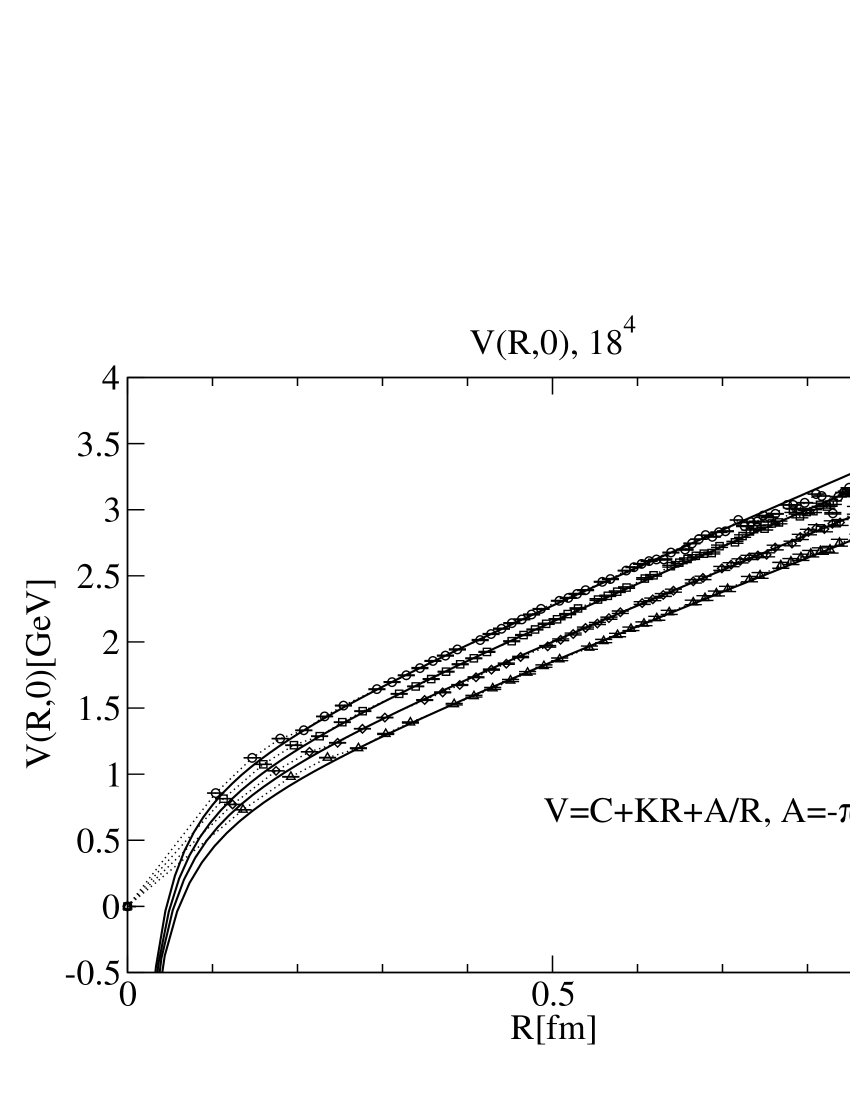
Figure 1: Coulomb heavy quark potentials obtained from the PPL correlator with $T=1$. These data were obtained in the $18^{4}$ lattice simulation at $\beta=5.85-6.00$. We used 400 gauge configurations measured every 100 sweeps.

Table 1: The fitting results for the string tensions. $K_{1}$ in lattice units and $\sigma_{1}$ in physical units were obtained from the singlet V(R,0). $K_{w}$ and $\sigma_{w}$ stand for the Wilson loop string tension at $\beta=6.0$ Bali (not calculated here). We use the relation $\sqrt{\sigma}=\sqrt{K}a^{-1}$ and the lattice cutoffs estimated with the Monte Carlo renormalization analyses qcdtaro .

$\beta$	$K_{1}$	$\sqrt{\sigma_{1}}$ [MeV]	$K_{w}$	$\sqrt{\sigma_{w}}$ [MeV]
5.85	0.2291(22)	706(4)
5.90	0.1950(10)	716(4)
5.95	0.1726(6)	736(3)
6.00	0.1467(4)	740(3)	0.0513(25) Bali	470(46)

Figure 1 shows the results of the Coulomb heavy quark potential $V(R,0)$ obtained from the PPL correlator with $T=1$. These data were obtained from the $18^{4}$ lattice simulations at $\beta=5.85-6.00$. To obtain the string tension, we assume the following fitting function:

$$V(R,T)=C+KR+A/R,\quad A=-\pi/12,$$ (13)

where $C$ is a constant and $K$ corresponds to the string tension. We find that the fittings are good; $\chi^{2}/ndf\sim O(1)$ for the fitting range $R=2-6$. It is found that the Coulomb heavy quark potential $V(R,0)$ rises linearly as the distance $R$ increases at $\beta=5.85-6.00$, and hence it can be described by the linear rise function with the string tension. The string tension for $\beta=5.85-6.00$ and the Wilson loop string tension Bali for $\beta=6.0$ are listed in Table LABEL:tab1. $K_{1}$ at $\beta=6.0$ is approximately three times larger than $K_{w}$, and the value of $\sqrt{\sigma_{1}}$ increases with $\beta$. Although similar results for the $\beta$ dependence of the string tension were also obtained in the $SU(2)$ lattice simulations Greensite ; Greensite2 , we have no clear explanation.

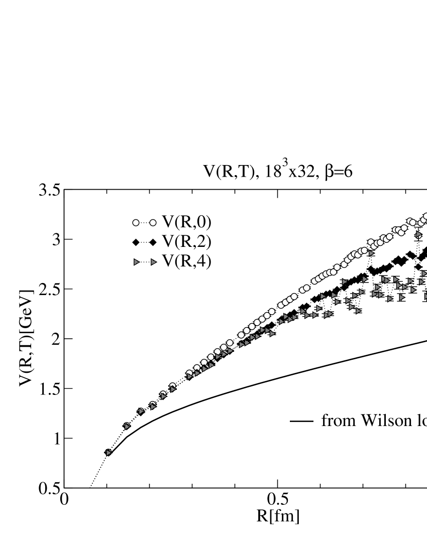
Figure 2: $T$ dependence of the Coulomb heavy quark potential at $\beta=6.0$. The symbols with error bars and the solid curve correspond to the numerical data calculated in the present work and using the Wilson-loop potential Bali , respectively. As $T$ increases, $V(R,T)$ seems to approach $V_{w}(R)$.

Because $V(R,T)$ in the limit $T\rightarrow\infty$ corresponds to a physical potential, we expect that $V(R,T)$ becomes comparable with the Wilson loop potential, $V_{w}(R)$, when $T$ becomes large enough. The $T$ dependence of the Coulomb heavy quark potential at $\beta=6.0$ is displayed in Fig. 2. We used the $18^{3}\times 32$ lattice and 600 configurations measured every 100 sweeps. $V(R,T)$ may approach $V_{w}(R)$ as $T$ increases. The $T$ dependence of the PPL correlator is not controlled completely here although there is consistency in the $SU(2)$ lattice calculations in Refs. Greensite and Greensite2 .

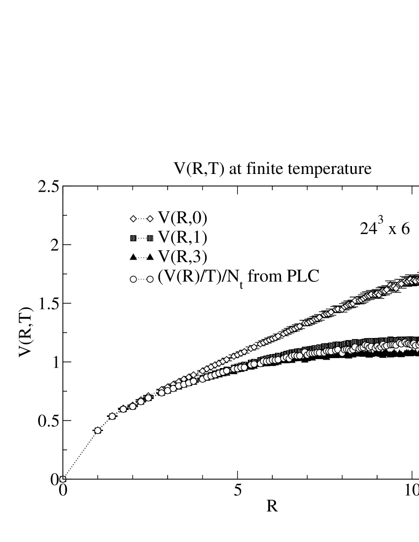
Figure 3: Linear-rise and screened potentials in the deconfinement phase at ${\cal T}/{\cal T}_{c}\sim 1.50$. Note that $V(R,0)$ still indicates linearly confining behavior, while the potentials $V(R,T)$ with finite $T$ are screened and are consistent with the calculation employing the usual full Polyakov-line correlator.

The finite temperature behavior of the Coulomb heavy quark potential is shown in Fig. 3. This simulation was carried out on the $24^{3}\times 6$ lattice at $\beta=6.11$ ($a\sim 0.086$ fm), corresponding to ${\cal T}/{\cal T}_{c}\sim 1.50$, where ${\cal T}$ stands for the system temperature and ${\cal T}_{c}$ the critical temperature of the quark-gluon plasma phase transition. The 300 configurations measured every 100 steps are used. It is very remarkable that even in the deconfinement region, ${\cal T}/{\cal T}_{c}\sim 1.50$, the Coulomb heavy quark potential $V(R,0)$ is not screened and still a linearly increasing function at large distances. Fitting these data with Eq. (13), we obtain $K_{1}(\beta=6.11,{\cal T}/{\cal T}_{c}\sim 1.50)$ = 0.118(1), and we find that $\sqrt{\sigma_{1}}(\beta=6.11,{\cal T}/{\cal T}_{c}\sim 1.50)$ = 792(10)MeV, which is larger than the value $\sqrt{\sigma_{1}}(\beta=6.0,{\cal T}\sim 0)$ = 740(4) MeV in Table LABEL:tab1; thus, it seems that the Coulomb string tensions with $T=1$ depend on QCD coupling $\beta$ rather than the system temperature ${\cal T}$. In the case of the color $SU(2)$ simulation, it is reported in Ref. Greensite2 that the Coulomb string tension scales well according to the two-loop $\beta$ function. On the other hand, as the temporal extension $T$ increases, the potential $V(R,T)$ are screened at large distances, $R\gtrsim 1/{\cal T}=6$ on this lattice, and they show the usual finite-temperature screening dynamics that have been investigated nonperturbatively in lattice simulations CDP1 ; SGluon .

III.2 Remnant symmetry in Coulomb gauge

We investigate the role of the remnant symmetry in Coulomb gauge. We calculate the order parameter $Q_{s}$ given in Eq. (10), and here we also study the color average order parameter

$$Q_{av}=\frac{1}{N_{t}}\sum_{t=1}^{N_{t}}\left<\sqrt{\frac{1}{3}\mbox{Tr}\tilde{U}(t)\mbox{Tr}{\tilde{U}^{\dagger}(t)}}\right>.$$ (14)

The volume dependence of the $Q$ values at zero temperature is shown in Fig. 4 and the simulation parameters are listed in Table 2. It is found that the $Q$ values vanish as $V_{s}\rightarrow\infty$. This indicates that the remnant symmetry is unbroken, and the system is in the confinement phase. The $Q$ values in the deconfinement phase are displayed in Fig. 5. The simulation parameters are also listed in Table 2. Figure 5 shows that the $Q$ values at finite temperature, ${\cal T}/{\cal T}_{c}\sim 1.26$, also go to zero as $V_{s}\rightarrow\infty$. It is found that the $Q$ values calculated here indicate no qualitative difference between the confinement and deconfinement phases in pure $SU(3)$ gauge theory; it is surprising that all the $Q$ values vanish as $V_{s}\rightarrow\infty$ even in the deconfinement phase, but this is a consequence of the fact that the Coulomb heavy quark potential $V(R,0)$ is always confining.

Table 2: Simulation parameters for the calculation of $Q_{av}$ and $Q_{s}$. All configuration measurements were performed every 10 steps.

$N_{s}^{3}\times 32$		$N_{s}^{3}\times 6$
$N_{s}$	No. of conf.	$N_{s}$	No. of conf.
8	100	18	100
18	100	24	90
24	100	42	30
32	30

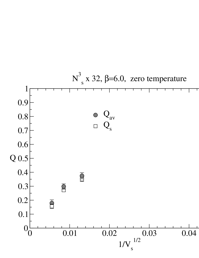
Figure 4: Volume dependence of $Q$ in the confinement phase at zero temperature. $Q_{s}$ and $Q_{av}$ vanish as $V\rightarrow\infty$.

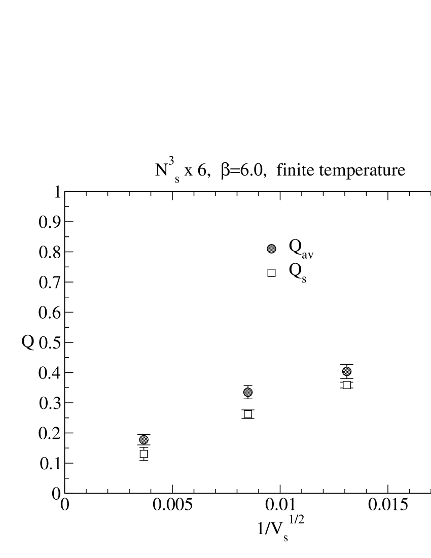
Figure 5: Volume dependence of $Q$ in the deconfinement phase at finite temperature, ${\cal T}/{\cal T}_{c}=1.26$. $Q_{s}$ and $Q_{av}$ vanish as $V\rightarrow\infty$.

III.3 Heavy quark potential in Lorentz gauge

Although the argument concerning the Coulomb heavy quark potential defined by the PPL correlator Greensite ; Greensite2 is based on use of Coulomb gauge, we carry out the same calculation in Lorentz gauge. The results are displayed in Fig. 6. This calculation was performed on the $24^{3}\times 32$ lattice at $\beta=6.0$, and 100 configurations measured every 100 steps are used.

The potential $V(R,0)$ in Lorentz gauge represents completely different behavior compared with the case of the Coulomb gauge. It is flat even at large distances. Moreover, as $T$ increases, the Lorentz heavy quark potential tends to approach the usual Wilson loop potential from below, but at large distances, the Lorentz heavy quark potential seems not to be confining. This strongly suggests that the color confinement mechanism is very different between Coulomb and Lorentz gauges.

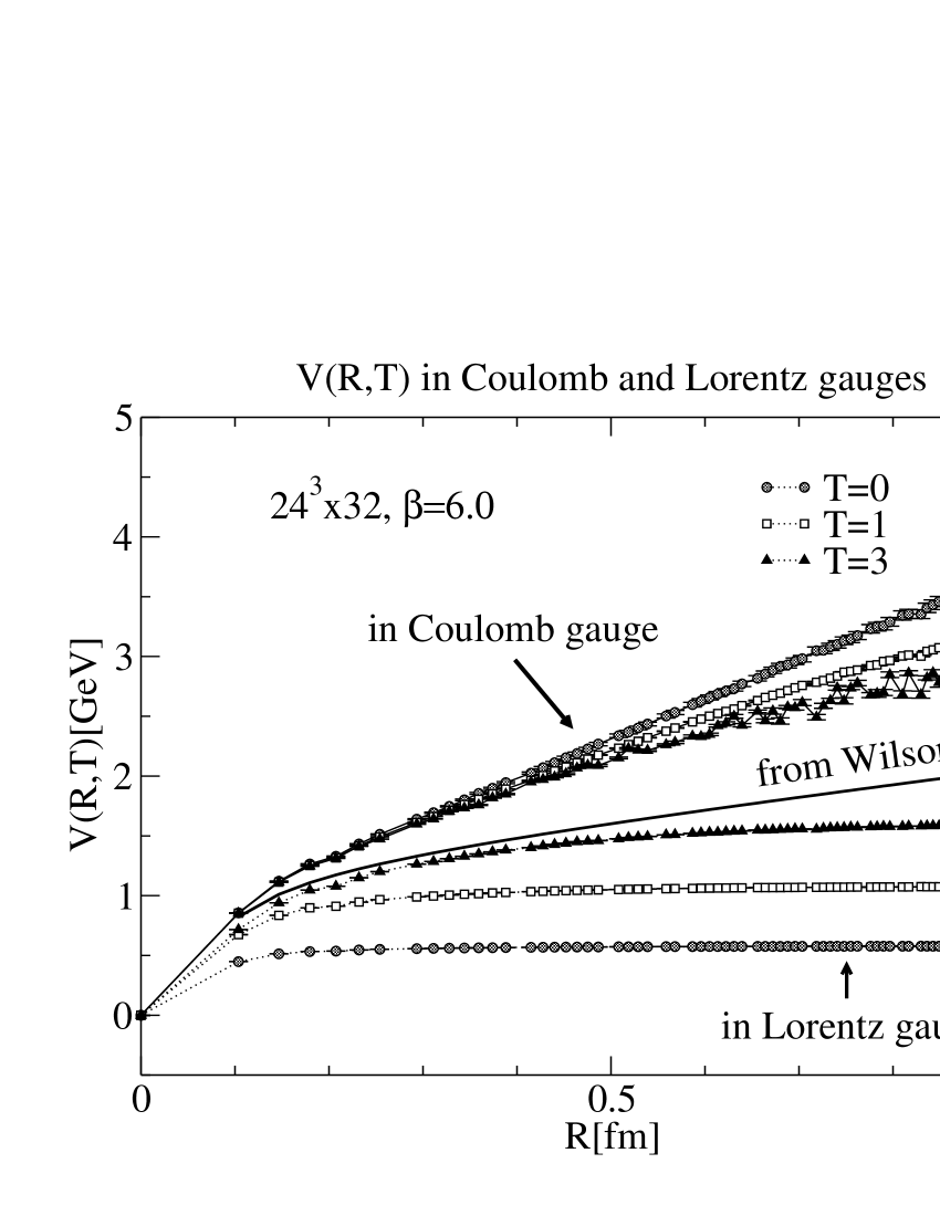
Figure 6: Heavy quark potentials in Coulomb and Lorentz gauges at $\beta=6.0$. The symbols with error bars represent the numerical data in Coulomb and Lorentz gauges, and the thick solid curve represents the Wilson loop potential at $\beta=6.0$.

IV Concluding remarks

We have nonperturbatively studied the long-range behavior of the Coulomb heavy quark potential defined by the partial-length Polyakov line correlators in quenched $SU(3)$ lattice gauge simulations. We confirmed numerically that the Coulomb heavy quark potential, corresponding to the color-Coulomb instantaneous part of the time-time gluon propagator, is confining, as suggested in the Coulomb confinement scenario CCG . The $SU(3)$ results obtained in this study are qualitatively consistent with those obtained in the $SU(2)$ analysis carried out by Greensite et al. Greensite ; Greensite2 . It is significant that we treated the instantaneous part nonperturbatively in the numerical simulations.

The Coulomb heavy quark potential $V(R,0)$ in the confinement phase rises linearly at large distances. Its string tension is several times larger than that obtained from the usual Wilson loop potential. As the temporal extension, $T$, of the PPL correlator, increases, the Coulomb heavy quark potential asymptotically approaches the usual Wilson loop potential. In these simulations, complete agreement is not confirmed. Note that consistency was found in the $SU(2)$ lattice gauge simulation Greensite . Furthermore, the result that the $SU(3)$ Coulomb heavy quark potential indicates a stronger confining property can be understood from the relation $V_{phys}(R)\leq V_{coul}(R)$Zwan .

The Coulomb string tension can also be estimated from lattice calculations of gluon propagators in Coulomb gauge. It is reported in Ref. CZproc that the Coulomb string tension $\sigma_{coul}\sim\sigma_{wilson}$. However, in the extensive lattice study of Langfeld and Moyaerts Langfeld , the authors concluded that the result $\sigma_{coul}\sim(2-3)\sigma_{wilson}$ cannot be ruled out. This observation is consistent with results derived in $SU(2)$ and $SU(3)$ lattice calculations with the PPL correlator.

In $SU(2)$ lattice simulations Greensite2 , $\beta$ dependence of the Coulomb string tension scales as a two-loop $\beta$ function. The Coulomb string tension measured here depends on the QCD coupling $\beta=6/g^{2}$. This $\beta$ dependence is not explicable here, and it is therefore desirable to verify it with numerical simulations in higher $\beta$ regions.

The Coulomb heavy quark potential $V(R,0)$ in the deconfinement phase at ${\cal T}/{\cal T}_{c}\sim 1.50$, also increases linearly with $R$ at large distances; i.e., it is not screened. However, the Coulomb heavy quark potential with the finite temporal length in Coulomb gauge is sufficiently screened, and finally it becomes comparable to the screened potentials obtained from the full temporal length Polyakov line correlator. This result may be explained in the Coulomb confinement scenario CCG ; renorm . $V(R,0)$ corresponds to the instantaneous part, $V_{coul}(R)\delta(t)$, and therefore $V_{coul}(R)$ does not depend on the time (temperature), whereas the non-instantaneous vacuum polarization term causes the time (temperature) dependent contribution.

We have also investigated the behavior of an order parameter related to the remnant symmetry in Coulomb gauge. As the lattice volume approaches infinity, the order parameter $Q$ vanishes in both the confinement and deconfinement phases. Thus, this order parameter is not a good parameter for understanding confinement physics, at least in pure $SU(3)$ gauge theory. This feature is a consequence of the fact that the Coulomb heavy quark potential is always confining in the confinement and deconfinement phases.

The Coulomb gauge plays an essential role in the confinement scenario discussed in Ref. CCG . We carried out the same calculation for the Lorentz gauge and found that the behavior of the Lorentz heavy quark potential is completely different from the case of Coulomb gauge. In Lorentz gauge, a different confinement scenario should be called for.

The color-Coulomb instantaneous part of the time-time gluon propagator exhibits color confinement. As discussed in Refs. CCG and renorm , this expectation may be satisfied in a dynamical-quark lattice simulation. The vacuum polarization causes a quark-pair creation at large quark separations, i.e. “string breaking”, whereas the Coulomb linear-rise potential also exists in that case. If one nonperturbatively extracts the contribution of the vacuum polarization, it may be easier to see the string breaking.

The color-Coulomb instantaneous part, $V_{coul}(R)\delta(t)$ or $V(R,0)$ on the fixed-time slice, shows the strong linear-rise behavior in $SU(2)$ and $SU(3)$ gauge theories at zero and finite temperatures; this phenomenon is as expected in view of the Coulomb confinement scenario CCG ; renorm . In terms of the Faddeev-Popov (FP) operator $M$, $V_{coul}(R)$ is given by $\langle M^{-1}(-\partial_{i}^{2})M^{-1}\rangle$, which has time-independent and long-range properties. According to the Gribov picture, gauge configurations for which the eigenvalues of the FP operator are small, i.e., regions near the Gribov horizon, play an important role in the confinement dynamics Gribov . Greensite et al. investigated eigenvalue distributions of the FP operator using the $SU(2)$ lattice gauge simulation FPeigen .

Here we concentrate on the Coulomb gauge. It would be interesting to study how the picture changes when we employ the other gauge by interpolating two gauges, such as $\sum_{i=1}^{3}\partial_{i}A_{i}+\lambda\partial_{t}A_{t}=0$IPG .

In this study, we use the gauge rotation, $e^{i\alpha\partial_{i}A_{i}}$, which is used in the stochastic gauge fixingSGF . This fixing term is “attractive” in the Gribov region and “repulsive” if one eigenvalue of the Faddeev-Popov operator is negative, and therefore the effect of Gribov copy may not be so serious. Nevertheless, it is important to study this point.

We investigated the behavior of the color-singlet $q\bar{q}$ potential in the present calculation. However, an extensive numerical study of the color-dependent forces between two quarks may be necessary to understand multiquark hadrons. In Coulomb gauge, $SU(3)$ color-dependent potentials have also been calculated in lattice gauge simulationszeroCDP .

It is interesting from a phenomenological point of view that the linearly rising behavior of the Coulomb potential exists even in the deconfinement phase at finite temperature. Therefore, a higher temperature simulation is indispensable and it may help to elucidate the behavior of the complex quark-gluon plasma system.

V Acknowledgments

We would like to thank D. Zwanziger for many helpful discussions and his continuous encouragement. We are also grateful to H. Toki for useful comments. The simulations were performed on an SX-5 (NEC) vector-parallel computer at the RCNP of Osaka University. We appreciate the support of the RCNP administrators. This work is supported by Grants-in-Aid for Scientific Research from Monbu-Kagaku-sho (No. 11440080, No. 12554008 and No. 13135216).

References

- (1) D. Zwanziger, Nucl. Phys. B 518 (1998) 237-272.
- (2) L. Baulieu, D. Zwanziger, Nucl.Phys. B548 (1999) 527-562, arXiv:hep-th/9807024.
- (3) A. Cucchieri and D. Zwanziger, Phys. Rev. D65 (2002) 014002, arXiv:hep-th/0008248.
- (4) D. Zwanziger, Phys. Rev. Lett. 90 (2003) 102001, arXiv:hep-lat/0209105.
- (5) A. Cucchieri and D. Zwanziger, Phys. Rev. D65 (2002) 014001, arXiv:hep-lat/0008026.
- (6) J. Greensite and Š. Olejník, Phys. Rev. D67, 094503 (2003), arXiv:hep-lat/0209068.
- (7) J. Greensite, Š. Olejník, D. Zwanziger, Phys. Rev. D69, 074506(2004), arXiv:hep-lat/0401003.
- (8) C. Feuchter and H. Reinhardt, Phys. Rev. D70, 105021(2004), arXiv:hep-th/0408236.
- (9) E. Marinari, M. L. Paciello, G. Parisi and B. Taglienti, Phys. Lett. B298 (1993), 400.
- (10) D. Zwanziger, Prog. Theor. Phys. Suppl. 131, 233 (1988), http://ptp.ipap.jp/link?PTPS/131/233/
- (11) J.E. Mandula and M. Ogilvie, Phys. Lett. B185 (1987) 127.
- (12) G. S. Bali, K. Schilling, Phys. Rev. D47 (1993) 661-672, arXiv:hep-lat/9208028.
- (13) K. Akemi, et al., QCDTARO Collaboration, Phys. Rev. Lett. 71 (1993) 3063, arXiv:hep-lat/9307004.
- (14) A. Nakamura, T. Saito, S. Sakai, Phys. Rev. D69 (2004) 014506, arXiv:hep-lat/0311024; A. Nakamura, et al., Phys. Lett. B549 (2002) 133-138, arXiv:hep-lat/0208075.
- (15) A. Nakamura and T. Saito, Prog.Theor.Phys. 112 (2004) 183-188, arXiv:hep-lat/0406038.
- (16) A. Nakamura and T. Saito, Prog.Theor.Phys. 111 (2004) 733-743, arXiv:hep-lat/0404002.
- (17) A. Cucchieri and D. Zwanziger, Nucl. Phys. B ( Proc. Suppl. ) 119 (2003) 727-729, arXiv:hep-lat/0209068.
- (18) K. Langfeld and L. Moyaerts, Phys. Rev. D70 (2004), 074507, arXiv:hep-lat/0406024.
- (19) V.N. Gribov, Nucl. Phys. B139, 1 (1978).
- (20) J. Greensite, Š. Olejník, D. Zwanziger, JHEP 0505 (2005) 070, arXiv:hep-lat/0407032.
- (21) C.S. Fischer and D. Zwanziger, Phys. Rev. D72 (2005) 054005, hep-ph/0504244.
- (22) D. Zwanziger, Nucl. Phys. B192, 259 (1981). ; E. Seiler, I.O. Stamatescu and D. Zwanziger, Nucl. Phys. B239, 177 (1984); A. Nakamura and M. Mizutani, Vistas in Astronomy (Pergamon Press), vol. 37, 305 (1993); M. Mizutani and A. Nakamura, Nucl. Phys. B(Proc. Suppl.) 34, 253 (1994).
- (23) A. Nakamura and T. Saito, Phys. Lett. B621 (2005) 171-175.