Embedded monopoles in quark eigenmodes
in SU(2) Yang-Mills Theory

Abstract

We study the embedded QCD monopoles (“quark monopoles”) using low-lying eigenmodes of the overlap Dirac operator in zero- and finite-temperature SU(2) Yang-Mills theory on the lattice. These monopoles correspond to the gauge-invariant hedgehogs in the quark-antiquark condensates. The monopoles were suggested to be agents of the chiral symmetry restoration since their cores should suppress the chiral condensate. We study numerically the scalar, axial and chirally invariant definitions of the embedded monopoles and show that the monopole densities are in fact globally anti-correlated with the density of the Dirac eigenmodes. We observe, that the embedded monopoles corresponding to low-lying Dirac eigenvalues are dense in the chirally invariant (high temperature) phase and dilute in the chirally broken (low temperature) phase. We find that the scaling of the scalar and axial monopole densities towards the continuum limit is similar to the scaling of the string-like objects while the chirally invariant monopoles scale as membranes. The excess of gluon energy at monopole positions reveals that the embedded QCD monopole possesses a gluonic core, which is, however, empty at the very center of the monopole.

I Introduction

It is generally believed ref:general:reviews:QCD ; ref:crossover:lattice:facts that the low-temperature (confinement) and the high-temperature (deconfinement) phases in QCD with realistic quark masses and vanishing chemical potential $\mu$ are separated by a smooth crossover which takes place at temperature $T_{c}\approx 170$ MeV. As the system goes through the crossover all thermodynamic quantities and their derivatives change smoothly, being non-singular functions of the temperature $T$. Therefore there is no local order parameter which can distinguish between these two phases at $\mu=0$.

Recently it was suggested ref:embedded:QCD that a well-defined boundary between the QCD phases at $\mu=0$ can still be rigorously defined as a proliferation (percolation) transition of the so-called “embedded QCD monopoles” or, as we also call them, “quark monopoles”. These monopoles are (gauge-invariant) composite objects made of quark and gluon fields. The monopoles are assumed to be proliferating at infinitely long distances in the high temperature phase while in the low-temperature phase they are moderately dilute. Contrary to Abelian monopoles in compact gauge theories, the embedded QCD monopoles are in general, not directly associated with the confining properties of the vacuum. The embedded monopoles can be considered as agents of the chiral symmetry restoration: in the low-temperature phase the chiral condensate should be suppressed in the cores of the embedded QCD monopoles while outside the monopoles the chiral condensate is suggested to be non-zero.

The assumption that the chiral phase transition should be driven by the percolation of such monopoles can intuitively be understood as follows ref:embedded:QCD . At low temperatures the density of the embedded monopoles is low and suppression of the chiral condensate by the monopole cores is negligibly small. However, as the temperature increases, the density of the embedded monopoles gets larger and, consequently, the chiral condensate becomes more suppressed. One can also look at the relation between the embedded monopole density and the chiral condensate from another side: with an increase of the temperature the chiral condensate becomes weaker, and the embedded monopoles – which are energetically unfavorable hedgehogs in the quark-antiquark condensates – become more populated. At some point the chiral condensate gets low enough for the embedded QCD monopoles to become sufficiently dense to start proliferating themselves.

The quark monopole in QCD is conceptually similar to the embedded defects of the Standard Electroweak (EW) model ref:semilocal:review . These defects are called as the Nambu monopoles ref:Nambu and the $Z$-vortices ref:Z:vortex . The $Z$–vortices (if they are not closed) begin and end on the Nambu monopoles. In the broken low-temperature phase the value of the Higgs field is suppressed inside the embedded EW defects, and is asymptotically non-zero outside the defects. According to analytical estimates Va94 the $Z$-vortices are proliferating for long distances in the high-temperature symmetric phase in which they form a dense percolating network. In the broken phase the $Z$-vortex network is destroyed and these objects become dilute. The Nambu monopoles possess similar properties ref:chernodub:nambu . Numerical simulations ref:hot:electroweak ; ref:Z:percolation show that the percolation transition of the $Z$-vortices takes place both at the region of the relatively small Higgs mass ref:hot:electroweak , $M_{H}\lesssim 72\,\mathrm{GeV}$, where the phase transition of the first order, and at large Higgs masses ref:Z:percolation , $M_{H}\gtrsim 72\,\mathrm{GeV}$, where the transition is a smooth analytical crossover ref:EW:phase .

In the condensed matter physics, an onset of percolation realized in the absence of a thermodynamic phase transition is usually referred to as the Kertész transition ref:Kertesz . The Ising model in an external magnetic field provides the best known example of the Kertész transition which is defined with respect to the so called Fortuin–Kasteleyn (FK) clusters ref:Fortuin:Kasteleyn . The FK clusters are sets of lattice links connecting nearest spins in the same spin states. These clusters are proliferating in the high temperature (disordered) phase and they are short-sized and dilute in the low temperature (ordered) phase. In zero magnetic field, $H=0$, the ordered and the disordered phases are separated by a phase transition at the Curie temperature $T_{c}$, which coincides with the percolation transition for the FK clusters. In an external magnetic field the phase transition is known to be absent and the ordered and disordered phases are connected analytically by a crossover in the $T$-$H$ plane. Nevertheless, the phases are still separated by a Kertész transition line $T_{K}=T_{K}(H)$ which marks the proliferation (percolation) transition for the FK clusters. Obviously, in the zero-field limit the Kertész line meets the Curie point, $\lim_{H\to 0}T_{K}(H)\to T_{c}$.

The Kertész-type transitions often appear in the gauge theories coupled to fundamental mater fields. Besides mentioned cases of embedded monopoles in QCD ref:embedded:QCD and the embedded defects in the Electroweak model ref:chernodub:nambu ; ref:hot:electroweak ; ref:Z:percolation , the Kertész line appears, for example, in the compact $U(1)$ gauge theories ref:Arwed . The manifestation of the Kertész line in the SU(2) Higgs model (which is similar to the Electroweak model) can be found as the percolation of the center vortices ref:Greensite:Faber .

The picture of percolating embedded monopoles in QCD is most probably related to the percolation of the hadron clusters at high temperature and non-zero density ($\mu\neq 0$) environment, which may be realized, for example, in the heavy-ion collision experiments. In these extreme conditions hadrons may overlap and form clusters within which the quarks are no more confined. The onset of the quark-gluon plasma phase is thus associated with the percolation transition of the hadron clusters ref:Satz:theory ; ref:Satz:percolation .

In this paper we study basic properties of the embedded (or, quark) monopoles using numerical simulations in the SU(2) gauge theory without dynamical matter field. The monopoles are defined with the help of $c$-valued eigenmodes of the overlap Dirac operator. In Section II we describe the structure of such monopoles in the continuum space-time. We show that in the SU(2) Yang-Mills theory there are three types of these monopoles characterized by their behavior with respect to the global axial transformations. We also discuss the extension of our construction to the realistic SU(3) case. In the same Section we provide a lattice construction of the quark monopoles, which is suitable for utilization in numerical simulations. In Section III we describe results of our numerical simulations for the density of the embedded monopoles. In Section IV we discuss a relation between the monopole density and the spectral density of the Dirac fermions. We also discuss a relation of our results to the Banks-Casher formula ref:Banks:Casher . Section V is devoted to numerical analysis of the structure of the chromomagnetic fields around the monopoles. Our conclusions are given in the last Section.

II Quark monopoles in continuum and on the lattice

The quark monopoles in QCD are analogues of the embedded (Nambu) monopoles ref:Nambu ; ref:semilocal:review in the Standard Electroweak model. Here we briefly outline the definition of the embedded QCD monopoles following Ref. ref:embedded:QCD . For the sake of simplicity we consider the gauge theory with the reduced number of colors, $N_{c}=2$. An outline of the generalization of our approach to the bigger number of colors is given at the end of this Section.

II.1 Quark monopoles in continuum SU(2) gauge theory

Let consider the SU(2) Yang-Mills theory with one (for simplicity) species of the fermion field $\psi$ which transforms in the fundamental representation of the gauge group. Using $\psi$ one can define the bilinear functions of the fermion field,

$$\vec{\xi}_{\Gamma}=\bar{\psi}(x)\Gamma\vec{\tau}\psi(x)\,,\qquad\Gamma={\mathchoice{\rm 1\mskip-4.0mul}{\rm 1\mskip-4.0mul}{\rm 1\mskip-4.5mul}{\rm 1\mskip-5.0mul}}\,,i\gamma_{5}\,,$$ (1)

where $\vec{\tau}=(\tau_{1},\tau_{2},\tau_{3})$ are the Pauli matrices acting in the color space and $\gamma_{\mu}$, $\gamma_{5}$ is the standard set of the spinor $\gamma$–matrices in the four-dimensional space-time. The real-valued composite fields $\vec{\xi}_{S}$ and $\vec{\xi}_{A}$ (with the subscripts $S$ and $A$ corresponding to the scalar, ${\mathchoice{\rm 1\mskip-4.0mul}{\rm 1\mskip-4.0mul}{\rm 1\mskip-4.5mul}{\rm 1\mskip-5.0mul}}$, and axial, $i\gamma_{5}$, operators, respectively) are scalar and, respectively, pseudoscalar (axial) fields from the point of view of space-time transformations. Both these fields transform as adjoint three-component quantities with respect to the action of the gauge group.

In the EW model the role of the adjoint composite field (1) is played by the scalar triplet $\Phi^{\dagger}\vec{\tau}\Phi$, where $\Phi$ is the two-component Higgs field. The EW embedded defects can then be formulated in terms of the classical or asymptotic configurations of the gauge and the Higgs fields. To make a tight link between the embedded defects in both theories we assume from the very beginning that the fermion field $\psi$ used in the definition (1) is a $c$-valued function. It is convenient to choose the field $\psi$ to be an eigenmode of the Dirac operator ${\cal D}$,

$${\cal D}[A]\psi_{\lambda}(x)=\lambda\psi_{\lambda}(x)\,,\qquad{\cal D}[A]=\gamma_{\mu}(\partial_{\mu}+i\frac{1}{2}\tau^{a}A^{a}_{\mu})+m\,,$$ (2)

corresponding to a configuration of the gauge fields $A^{a}_{\mu}(x)$. In our numerical analysis we use the massless Dirac operator with $m=0$. The Dirac eigenmodes are labeled by the eigenvalues $\lambda$ of the Dirac operator. The label $\lambda$ will be omitted in this Section for the sake of simplicity.

The axial transformations are defined by the global Abelian parameter $\alpha$,

$$U_{A}(1):\qquad\psi\to e^{i\alpha\gamma_{5}}\psi\,,\quad\bar{\psi}\to\bar{\psi}e^{i\alpha\gamma_{5}}\,.$$ (3)

The color vectors $\vec{\xi}_{S}$ and $\vec{\xi}_{A}$ are transforming into each other under the axial transformations (3) as follows:

$$\left(\begin{array}[]{c}\vec{\xi}_{S}\\ \vec{\xi}_{A}\end{array}\right)\to{\left(\begin{array}[]{c}\vec{\xi}_{S}\\ \vec{\xi}_{A}\end{array}\right)}^{\prime}=\left(\begin{array}[]{cc}\cos 2\alpha&\sin 2\alpha\\ -\sin 2\alpha&\cos 2\alpha\end{array}\right)\left(\begin{array}[]{c}\vec{\xi}_{S}\\ \vec{\xi}_{A}\end{array}\right)\,.$$ (12)

Using two adjoint fields (1) we define three unit color vectors

$$\vec{n}_{S}=\frac{\vec{\xi}_{S}}{|\vec{\xi}_{S}|}\,,\quad\vec{n}_{A}=\frac{\vec{\xi}_{A}}{|\vec{\xi}_{A}|}\,,\quad\vec{n}_{I}=\frac{\vec{\xi}_{S}\times\vec{\xi}_{A}}{|\vec{\xi}_{S}\times\vec{\xi}_{A}|}\,,$$ (13)

where $(\vec{A},\vec{B})$ and $[\vec{A}\times\vec{B}]^{a}=\epsilon^{abc}A^{b}B^{c}$ are, respectively, the scalar and the vector products in the color space and $|\vec{A}|=(\vec{A},\vec{A})^{1/2}$ is the norm of the color vector $A$. The last term in Eq. (13), $\vec{n}_{I}$, is a (normalized) vector product of the scalar and axial color vectors. The vector $\vec{n}_{I}$ is interesting because it is invariant under the axial transformations (3), (12). The index $I$ in the subscript of $\vec{n}_{I}$ stands for ”invariant”.

The crucial observation is to interpret the unit vectors (13) as directions of the corresponding composite adjoint Higgs field. Thus we have three Georgi-Glashow multiplets $(n^{a}_{\Gamma},A^{a}_{\mu})$, $\Gamma=S,A,I$, which can be used to construct the gauge invariant ’t Hooft tensors ref:thooft ,

$${\cal F}^{\Gamma}_{\mu\nu}(n_{\Gamma},A)=F^{a}_{\mu\nu}(A)\,n_{\Gamma}^{a}-\frac{1}{g}\epsilon^{abc}n_{\Gamma}^{a}{(D^{\mathrm{ad}}_{\mu}n_{\Gamma})}^{b}{(D^{\mathrm{ad}}_{\nu}n_{\Gamma})}^{c}\,,\qquad\Gamma=S\,,A\,,I\,,$$ (14)

where $F^{a}_{\mu\nu}=\partial_{\mu}A^{a}_{\nu}-\partial_{\nu}A^{a}_{\mu}+g\epsilon^{abc}A^{b}_{\mu}A^{c}_{\nu}$ is the field strength tensor for the SU(2) gauge field $A^{a}_{\mu}$, and

$${(D^{\mathrm{ad}}_{\mu})}^{ab}=\delta^{ab}\,\partial_{\mu}+g\,\epsilon^{abc}A^{c}_{\mu}\,,$$ (15)

is the adjoint covariant derivative. The ’t Hooft tensor (14) is the gauge-invariant field strength tensor for the diagonal (with respect to the color direction $\vec{n}_{\Gamma}$) component of the gauge field,

$${\cal A}^{\Gamma}_{\mu}=A^{a}_{\mu}n^{a}_{\Gamma}\,,\qquad\Gamma=S\,,A\,,I\,.$$ (16)

The current of the quark monopole of the $\Gamma^{\mbox{th}}$ type,

$$k^{\Gamma}_{\nu}=\frac{g}{4\pi}\partial_{\mu}\tilde{\cal F}^{\Gamma}_{\mu\nu}\equiv\int_{{\cal C}^{\Gamma}}d\tau\frac{\partial X^{{\cal C}^{\Gamma}}_{\nu}(\tau)}{\partial\tau}\,\delta^{(4)}(x-X^{{\cal C}^{\Gamma}}(\tau))\,,\qquad\tilde{\cal F}^{\Gamma}_{\mu\nu}=\frac{1}{2}\epsilon_{\mu\nu\alpha\beta}{\cal F}^{\Gamma}_{\alpha\beta}\,,$$ (17)

has a $\delta$–like singularity at the corresponding worldline ${\cal C}^{\Gamma}$. The monopole worldline is parameterized by the vector $x_{\mu}=X^{{\cal C}^{\Gamma}}_{\mu}(\tau)$ and the parameter $\tau$. The quark monopoles defined according to Eq. (17) are quantized and the corresponding monopole charge is conserved (i.e., the worldlines ${\cal C}^{\Gamma}$ are closed).

The quark monopoles $k^{\Gamma}_{\mu}$ carry the magnetic charges with respect to the “scalar”, “axial” and “chirally invariant” components of the gauge field ${\cal A}^{\Gamma}_{\mu}$, Eq. (16). In the corresponding Unitary gauges $n^{a}_{\Gamma}=\delta^{a3}$, the quark monopoles correspond to monopoles “embedded” into the diagonal component (16). In the gauges, where the diagonal component ${\cal A}^{\Gamma}_{\mu}$ is regular, such monopoles are hedgehogs in the composite quark-antiquark fields. The corresponding quark condensates are characterized by the typical hedgehog behavior $n^{a}_{\Gamma}\sim x^{a}$ in the local (transverse) vicinity of the monopoles. The fact of the existence of these monopoles in QCD is not a dynamical fact but rather a simple (kinematical) consequence of the existence of the adjoint real-valued fields (1), (13). Note that there is an infinite number of equivalent formulations of the embedded monopoles associated with triplet isovectors which are given by a chiral rotation (12) of, say, isovector $\vec{\xi}_{A}$ with an arbitrary angle $\alpha$. The dynamics of these monopoles is studied below.

Let us summarize briefly: if one has the configuration of the gauge field $A_{\mu}$ and the configuration of the (generally massive) quark $c$-field $\psi$ then the location of the embedded quark monopoles of all three types (“scalar”, “axial” and “invariant”) can be found with the help of relations (1), (13), (14), (17). The quark $c$-fields $\psi$ can be defined as a set of eigenmodes of the Dirac operator (2), labeled by the eigenvalue $\lambda$.

II.2 Quark monopoles in SU(2) gauge theory on the lattice

The lattice construction of the quark monopoles in Euclidean QCD closely resembles a similar lattice construction ref:sphaleron of the embedded defects in the standard model of electroweak interactions. Consider a configuration of the lattice gauge fields $U(x,\mu)$ and a configuration of the $c$-valued fermion matter field $\Psi(x)$. Using the fermionic field $\Psi(x)$ one can construct the composite color fields on the Euclidean lattice,

$$\xi^{a}_{S}(x)=\Psi^{\dagger}(x)\tau^{a}\Psi(x)\,,\qquad\xi^{a}_{A}(x)=\Psi^{\dagger}(x)\tau^{a}\gamma_{5}\Psi(x)\,,$$ (18)

which are the lattice analogues of the continuum expressions (1). Then the adjoint variables $\xi^{a}_{S}$ and $\xi^{a}_{A}$ can be used to construct the lattice unit vectors $n_{S}$, $n_{A}$, and $n_{I}$, in a manner completely similar to Eq. (13).

The next step is to define the (un-normalized) projections of the gauge field onto the color directions $n_{\Gamma}\equiv n^{a}_{\Gamma}\tau^{a}$:

$$V_{\Gamma}(x,\mu)=U(x,\mu)+n_{\Gamma}(x)U(x,\mu)n_{\Gamma}(x+\hat{\mu})\,,\qquad\Gamma=S\,,A\,,I\,.$$

The field $V_{\Gamma}$ behaves under the action of the gauge transformation $\Omega$ as a gauge field,

$$V_{\Gamma}(x,\mu)\to\Omega^{\dagger}(x)V_{\Gamma}(x,\mu)\Omega(x+\hat{\mu})\,.$$

The lattice analogue of the ’t Hooft tensor (14) is given ref:sphaleron by the compact field ${\bar{\theta}}(x,\mu\nu)\in(-\pi,\pi]$ defined on the plaquette $P=\{x,\mu\nu\}$:

$${\bar{\theta}}^{\Gamma}(x,\mu\nu)=\arg\Bigl{(}{\mathrm{Tr}}\left\{\Bigl{[}{\mathchoice{\rm 1\mskip-4.0mul}{\rm 1\mskip-4.0mul}{\rm 1\mskip-4.5mul}{\rm 1\mskip-5.0mul}}+n_{\Gamma}(x)\Bigr{]}V_{\Gamma}(x,\mu)V_{\Gamma}(x+\hat{\mu},\nu)V^{\dagger}_{\Gamma}(x+\hat{\nu},\mu)V^{\dagger}_{\Gamma}(x,\nu)\right\}\Bigr{)}\,.$$ (19)

Due to the property $n_{\Gamma}(x)V_{\Gamma}(x,\mu)=V_{\Gamma}(x,\mu)n_{\Gamma}(x+\hat{\mu})$, the definition (19) is independent of the choice of the reference point $x$ on the plaquette $P$. One can show that in the Unitary gauge, $n_{\Gamma}(x)=\tau^{3}$, the gauge invariant plaquette function (19) coincides with the standard Abelian plaquette formed out of the compact Abelian fields $\theta^{u}_{\Gamma}(x,\mu)={\mathrm{arg}}\,U^{11}_{\Gamma}(x,\mu)$.

The singularities in the compact fields ${\bar{\theta}}_{\Gamma}$ correspond to the quark monopoles of the scalar, axial and invariant types. The quark monopoles are defined on the links of dual lattice $\mbox{}^{\ast}\{x,\mu\}$ which are dual to the cubes $c_{x,\mu}$ of the primary lattice:

$$j^{\Gamma}(x,\mu)=-\frac{1}{2\pi}\sum_{P\in\partial c_{x,\mu}}{\bar{\theta}}^{\Gamma}_{P}\,,$$ (20)

where the sum is taken over all six plaquettes $P$ forming the faces of the cube $c_{x,\mu}$. Equation (20) is an analog of the standard definition DGT of the Abelian monopole in the lattice gauge theory of compact Abelian fields. By construction, the monopole current (20) is integer-valued, $j^{\Gamma}\in{Z\!\!\!Z}$, and conserved, $\delta\mbox{}^{\ast}j^{\Gamma}=0$. Here the operator $\delta$ is the lattice divergence.

II.3 Generalization to SU(3) gauge group

The construction of the embedded quark monopoles can be generalized to the realistic case of the $SU(3)$ Yang-Mills theory. The structure of such monopoles shares similarity with the non-Abelian monopoles in the $SU(3)$ gauge theory coupled to an octet Higgs field. A good review of the subject on the monopole configurations in the $SU(3)$ gauge-Higgs models be found in Refs. ref:Yasha . Below we briefly outline the construction to be discussed elsewhere in more detail ref:chernodub:inpreparation .

The generators of the $SU(3)$ gauge group are given by eight traceless matrices $T^{a}=\lambda^{a}/2$ normalized as ${\mathrm{T}r}T^{a}T^{b}=\delta^{ab}/2$. Here $\lambda^{a}$ are the standard Gell-Mann matrices. Contrary to the simplest case of two colors, there are two structure constants in the $SU(3)$ gauge group. The totally symmetric constant $f^{abc}$ is defined via the relation $[T^{a},T^{b}]=if^{abc}T^{c}$, while the values of the totally symmetric structure $d^{abc}$ can be deduced from the equation $\{T^{a},T^{b}\}=\frac{1}{3}\delta^{ab}+d^{abc}T^{c}$. These constants can also be expressed via the single relation, $4{\mathrm{T}r}T^{a}T^{b}T^{c}=d^{abc}+if^{abc}$.

Similarly to the $SU(2)$ case (1) the $SU(3)$ model admits two composite octet vectors

$$\xi^{a}_{\Gamma}=\bar{\psi}(x)\Gamma\vec{T}^{a}\psi(x)\,,\qquad\Gamma={\mathchoice{\rm 1\mskip-4.0mul}{\rm 1\mskip-4.0mul}{\rm 1\mskip-4.5mul}{\rm 1\mskip-5.0mul}}\,,i\gamma_{5}\,,$$ (21)

where we use the same notations as in the $SU(2)$ case. This should not, however, lead to a confusion since the $SU(3)$ gauge group is discussed in this Section only.

Besides the scalar octet $\xi^{a}_{S}$ with $\Gamma={\mathchoice{\rm 1\mskip-4.0mul}{\rm 1\mskip-4.0mul}{\rm 1\mskip-4.5mul}{\rm 1\mskip-5.0mul}}$ and the axial octet $\xi^{a}_{A}$ with $\Gamma=i\gamma_{5}$ the structure $SU(3)$ gauge group allows us to build the invariant field

$$\xi^{a}_{I}=f^{abc}\xi^{b}_{S}\xi^{b}_{A}\,,$$ (22)

which transforms in the adjoint representation of the $SU(3)$ gauge group. The octet $\xi_{I}$ is the $SU(3)$ generalization of the invariant $SU(2)$ triplet field $\xi_{I}=\vec{\xi}_{S}\times\vec{\xi}_{A}$ which is used in Eq. (13). One can explicitly show that the composite field (22) is invariant under the global axial rotations which read in terms of the $SU(3)$ octet fields (21) as follows:

$$\xi^{a}_{\Gamma}\to R_{\Gamma\Gamma^{\prime}}\xi^{a}_{\Gamma^{\prime}}\,,\qquad R=\left(\begin{array}[]{cc}\cos 2\alpha&\sin 2\alpha\\ -\sin 2\alpha&\cos 2\alpha\end{array}\right)\left(\begin{array}[]{c}\xi^{a}_{S}\\ \vec{\xi}^{a}_{A}\end{array}\right)\,,\qquad\Gamma,\Gamma^{\prime}=S,A\,.$$ (27)

In addition to the asymmetric constant $f^{abc}$ the $SU(3)$ gauge group possess the symmetric structure constant $d^{abc}$. Therefore one can define three additional octet fields, $\xi^{a}_{SS}$, $\xi^{a}_{AS}\equiv\xi^{a}_{SA}$ and $\xi^{a}_{AA}$ which form a symmetric rank-2 tensor field,

$$\xi^{a}_{\Gamma_{1}\Gamma_{2}}=d^{abc}\xi^{b}_{\Gamma_{1}}\xi^{b}_{\Gamma_{2}}\,,\qquad\Gamma_{1,2}=S,A\,,$$ (28)

with respect to the global axial rotations (27):

$$\xi^{a}_{\Gamma_{1}\Gamma_{2}}\to R_{\Gamma_{1}\Gamma^{\prime}_{1}}R_{\Gamma_{2}\Gamma^{\prime}_{2}}\xi^{a}_{\Gamma^{\prime}_{1}\Gamma^{\prime}_{2}}\,.$$ (29)

Summarizing, in the realistic case of three colors we have six independent structures which are classified with respect to the global axial rotations (27) as the scalar ($\xi^{a}_{I}$), vector ($\xi^{a}_{S}$ and $\xi^{a}_{A}$), and rank-2 symmetric tensor ($\xi^{a}_{SS}$, $\xi^{a}_{SA}$, and $\xi^{a}_{AA}$). All these structures behave as octet fields with respect to the $SU(3)$ gauge transformations.

Note, that from a kinematical point of view any of the six octet fields can equivalently be used to construct the embedded quark monopoles in the $SU(3)$ gauge theory. The relevance of one or another octet field is to be figured out with the help of the dynamical considerations (i.e., with the help of numerical simulations). In the rest of this Section we describe the kinematical construction of the embedded monopoles in the theory with the $SU(3)$ gauge group and therefore use a generic notation $\xi^{a}$ for any of the six composite fields, or for a linear combinations of them.

In order to characterize the embedded monopoles in QCD it is convenient to work in the Cartan-Weyl basis ref:Weinberg . The Cartan subgroup of the $SU(3)$ gauge group is generated by two diagonal generators

$$H_{1}\equiv T^{3}=\frac{1}{2}\left(\begin{array}[]{rrr}1&0&0\\ 0&-1&0\\ 0&0&0\\ \end{array}\right)\,,\quad H_{2}\equiv T^{8}=\frac{1}{2\sqrt{3}}\left(\begin{array}[]{rrr}1&0&0\\ 0&1&0\\ 0&0&-2\\ \end{array}\right)\,,$$ (36)

which form the two-component vector $\vec{H}=(H_{1},H_{2})$. In any point of the space-time the octet field $\xi^{a}$ can be gauge-rotated to the Cartan subalgebra

$$\Phi(x)\to|\Phi(x)|\,(\vec{h}(x),\vec{H})\,,\quad\vec{h}^{2}=1\,.$$ (37)

where $(a,b)$ denotes the scalar product in the Cartan space, and $\vec{h}$ is the unit two-component vector pointing to the direction of the composite octet field $\xi$ in the Cartan space.

The magnetic charge of the $SU(3)$ monopole ref:Weinberg

$${\vec{g}}_{M}=\frac{4\pi}{g}\Bigl{(}n_{1}{\vec{\beta}}^{*}_{1}+n_{2}{\vec{\beta}}^{*}_{2}\Bigr{)}\,,$$ (38)

is given in terms of the dual simple roots ${\vec{\beta}}^{*}_{\alpha}$ with $\alpha=1,2$. The dual roots ${\vec{\beta}}^{*}_{\alpha}$ are expressed in terms of the original simple roots ${\vec{\beta}}_{\alpha}$ of the $SU(3)$ group as ${\vec{\beta}}^{*}_{\alpha}={\vec{\beta}}_{\alpha}/|{\vec{\beta}}_{\alpha}|^{2}$. These roots are often chosen in the self-dual form,

$${\vec{\beta}}_{1}=(1,0)\,,\qquad{\vec{\beta}}_{2}=(-1/2,\sqrt{3}/2)\,.$$ (39)

The generalization of the standard Dirac quantization of the monopole charge to the case of the $SU(3)$ monopole reads as

$$e^{ig(\vec{g}_{M},\vec{H})}={\mathchoice{\rm 1\mskip-4.0mul}{\rm 1\mskip-4.0mul}{\rm 1\mskip-4.5mul}{\rm 1\mskip-5.0mul}}\,.$$ (40)

The Dirac condition (40) is satisfied by Eq. (38) provided the numbers $n_{1}$ and $n_{2}$ are integer.

The classification of the $SU(3)$ monopoles qualitatively depends on the direction of the local Higgs field in the Cartan subalgebra. If the vector $\vec{h}$ in Eq. (37) is not orthogonal to any of the simple roots $\vec{\beta}_{1}$ and $\vec{\beta}_{2}$, Eq. (39), then the pattern of the symmetry breaking is “maximal” ref:Weinberg

$$SU(3)\to U(1)\times U(1)\,,$$ (41)

and the corresponding vacuum manifold is characterized by a non-trivial second homotopy group,

$$\pi_{2}\left(\frac{SU(3)}{U(1)\times U(1)}\right)={\mathbb{Z}}^{2}\,.$$ (42)

Thus, the monopoles are described by the two integer numbers. These numbers are $n_{1}$ and $n_{2}$ which enter the definition of the monopole charge (38).

If the asymptotic Higgs field is orthogonal either to the simple root $\vec{\beta}_{1}$ or to the simple root $\vec{\beta}_{2}$, then the symmetry breaking is “minimal”

$$SU(3)\to U(2)\,.$$ (43)

This pattern also possess a non-trivial second homotopy group,

$$\pi_{2}\left(\frac{SU(3)}{U(2)}\right)={\mathbb{Z}}\,,$$ (44)

and the monopoles are characterized by one integer number which is either $n_{1}$ (if $(\vec{\beta}_{2},\vec{h})=0$) or $n_{2}$ (if $(\vec{\beta}_{1},\vec{h})=0$).

The position of the $SU(3)$ monopole can locally be determined with the help of the ’t Hooft tensors similarly to the $SU(2)$ case (17). In the Cartan space the monopole is a point-like source of the magnetic field which is described locally as ${\mathbf{B}}\simeq({\vec{g}}_{M},\vec{H}){\mathbf{r}}/r^{3}$ provided ${\vec{r}}$ is close to the center of the monopole. The type of the symmetry breaking pattern corresponds to the type of the embedding of the $SU(2)$ HP monopole into the larger $SU(3)$ group. In the general case of the $SU(N)$ gauge group the embedded monopoles can be formulated similarly to the case of the $SU(N)$ gauge-Higgs monopoles reviewed in detail in Ref. ref:Yasha .

It is known ref:Yasha that in the case of the monopole-like solutions to the classical equations of motion of the $SU(3)$ gauge-Higgs model, the choice of either maximal (41) or minimal (43) symmetry breaking patterns depends on the details of the Higgs potential ref:Yasha . In the case of QCD one can realize both patterns simultaneously. Let us take any of the six octet fields (21), (22) or (28), and project it onto the Cartan subgroup . The color direction of this field in any point is usually not perpendicular to any of the root vectors (39) apart from rare degenerate cases. Thus, if we choose any of the above octets as the effective Higgs field $\xi$, then it is likely that the maximal embedding pattern (41) is realized. On the other hand, a linear combination of any of the two octets can always be fine-tuned (again, apart from rare degenerate cases) to be perpendicular to a chosen root vector, so that the minimal embedding pattern (43) can also be realized in QCD. A discussion on the kinematical construction and well as on the possible dynamical significance of such monopoles in QCD will be published elsewhere ref:chernodub:inpreparation . Below we discuss numerical signatures of the embedded quark monopoles in the simpler case with two colors.

III Density of quark monopoles at zero and finite temperature

In order to study basic properties of the embedded QCD monopoles we perform a simulation of the pure SU(2) Yang-Mills model on the lattice at zero and finite temperatures. The technical details of numerical simulations are given in Appendix A, and below we discuss the results of the simulations.

III.1 Monopole densities and the effect of temperature

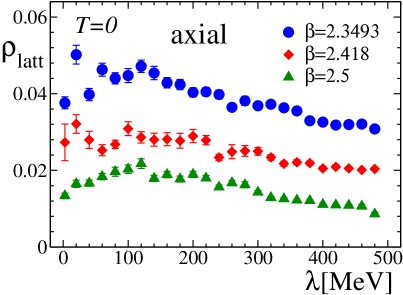
(a)	(b)
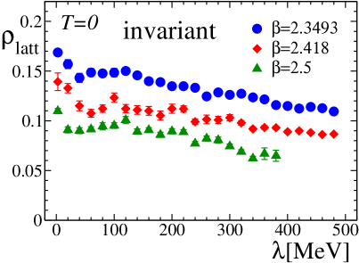
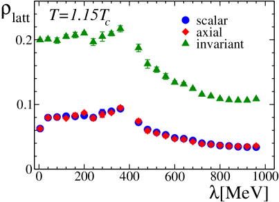
(c)	(d)

Figure 1: (Color online) The densities of the (a) scalar, (b) axial, and (c) chirally invariant embedded monopoles in confinement phase for $\beta=2.3493$, $2.418$, and $2.5$ on vs. the Dirac eigenvalue $\lambda$. (d) The same but for the deconfinement phase at $T=1.15T_{c}$. The densities are given in the units of the lattice spacing $a$.

In Figures 1 (a), (b) and (c) we show the lattice densities $\rho_{{\mathrm{latt}}}$ of, respectively, scalar, axial and invariant embedded monopoles at zero temperature. The densities, plotted in the units of the lattice spacing $a$, are shown as functions of the Dirac eigenmode energy $\lambda$ for three values of the coupling $\beta$. Apart from a few irregular points (which we ascribe to statistical fluctuations), the densities are smooth functions of the eigenmode energy $\lambda$. Moreover the scalar and axial densities at zero-temperature are decreasing functions of $\lambda$ for $\lambda\gtrsim 150\,\mbox{MeV}$. The density of the chirally invariant quark monopole is a decreasing function for all considered values of $\lambda$. The density of the chirally invariant monopoles is higher than the scalar and axial monopole densities.

According to Figures 1 (a) and (b) the scalar and axial densities coincide with each other within the error bars. This observation does not contradict the statement that the chiral symmetry is broken in the low-temperature phase. In order to illustrate this fact let us consider, as a toy example, a lattice model describing the $SO(2)$ global scalar field $\phi=(\phi_{1},\phi_{2})^{T}$ with two real-valued components $\phi_{1}$ and $\phi_{2}$. The global $SO(2)$ symmetry treats the field $\phi$ as a two-component vector in an internal space. This symmetry is an analogue of the axial symmetry (3), while the components $\phi_{1}$ and $\phi_{2}$ can be associated with the scalar, $\xi_{S}$, and axial, $\xi_{A}$, triplets, respectively.

Apart from a kinetic term, $(\partial_{\mu}\phi)^{2}$, a generic Lagrangian of the toy model should contain the $SO(2)$-invariant potential

$$V(\phi^{2})=\mu^{2}\phi^{2}+\lambda(\phi^{2})^{2}\,,$$ (45)

with $\phi^{2}\equiv\phi^{2}_{1}+\phi^{2}_{2}$. In the broken phase ($\mu^{2}<0$) the scalar field develops a non-zero expectation value in the infinite volume system, $\langle\phi\rangle\neq 0$. As a consequence, the vacuum of the model becomes non-invariant under the $SO(2)$ transformations. In the symmetric phase ($\mu^{2}\geqslant 0$) the global symmetry is restored since $\langle\phi\rangle=0$.

However, in a finite volume the expectation values of the components of the Higgs fields should vanish in both phases, $\langle\phi_{1}\rangle_{V}=0$ and $\langle\phi_{2}\rangle_{V}=0$ (here the subscript $V$ in $\langle\dots\rangle_{V}$ indicates that the averages are taken in a finite volume). This happens because in the averages the finite number of integrals over the scalar fields $\phi_{1,2}(x)$ includes also integrations over all orientations of the fields in the internal space. Thus, in a finite-element system all the internal directions are formally equivalent. Moreover, one gets $\langle\phi^{2}_{1}\rangle_{V}\equiv\langle\phi^{2}_{1}\rangle_{V}$ both in broken and unbroken phases because of the same reason. This is precisely the same what we could expect for the expectation values of the triplet fields, $\langle\vec{\xi}^{2}_{S}\rangle_{V}=\langle\vec{\xi}^{2}_{A}\rangle_{V}$, in a finite volume system regardless if the chiral symmetry is broken in the thermodynamic limit or not.

As a consequence, finite volume expectation values of any operator ${\mathcal{O}}(\xi_{S})$ should be equivalent to the expectation value of its axial counterpart ${\mathcal{O}}(\xi_{A})$. In other words, the choice of the axial isovector $\vec{\xi}_{A}$ in a role of the adjoint composite Higgs field is as good as the choice of the scalar isovector $\vec{\xi}_{S}$. Thus the densities of the scalar and axial quark monopoles should coincide with each other in the finite volume.

Apart from the quenched case, in the real QCD with dynamical quarks the breaking of the chiral symmetry must explicitly be seen in the densities of the embedded monopoles: the density of the scalar and axial monopoles must in general be different. For example, it is expected ref:embedded:QCD that at sufficiently high temperatures the density of the axial quark monopoles should be higher than the density of the scalar monopoles. We expect that the effect should also be observable in the finite volume because of an explicit breaking of the axial symmetry by the fermion determinant. In fact, the measure of the integration over the fermion fields is axially anomalous ref:Fujikawa , and therefore the expectation values of the operator ${\mathcal{O}}(\xi_{S})$ should be different from its axial analogue ${\mathcal{O}}(\xi_{A})$. In terms of the toy $SO(2)$ model the effect of non-invariant measure can be emulated by an addition of an extra $SO(2)$ breaking term (say $\delta V\propto\phi_{1}$) to the potential (45).

In Figure 1 (d) we show the density of the quark monopoles at the temperature $T=1.15\,T_{c}$ corresponding to the deconfinement phase. Similarly to the zero temperature case, the density of the scalar and axial monopoles coincide with each other. The invariant monopoles are denser than the scalar/axial monopoles for all values of eigenvalue $\lambda$. The monopole density is independent of the eigenvalue in the region $0\leqslant\lambda\lesssim 400\,\mbox{MeV}$. In the limit $\lambda\to 0$ the densities of the scalar/axial and invariant monopoles in physical units are, respectively,

$$\lim_{\lambda\to 0}\rho^{\mathrm{phys}}_{\Gamma}(\lambda)\to\left\{\begin{array}[]{ll}\approx{(3\,\mathrm{fm})}^{3}&\quad\mbox{[scalar and axial]}\\ \approx{(4\,\mathrm{fm})}^{3}&\quad\mbox{[invariant]}\end{array}\right.\quad\qquad\quad T=1.15\,T_{c}\,.$$ (48)

In the region $\lambda\gtrsim 400\,\mbox{MeV}$ the density of the monopoles of all three types quickly drops down. This observation will be confronted with the fermion spectral function in Section IV.

To estimate the effect of temperature on the monopole density it worth comparing the lattice monopole densities at zero temperature for $\beta=2.3493$ (shown by filled circles in Figures 1(a),(b), and (c)) and at $T=1.15\,T_{c}$ for $\beta=2.35$ (shown in Figure 1(d)). The selected values of the lattice coupling $\beta$ are very close to each other and therefore they correspond to almost the same value of the lattice spacing $a$ according to Table 1 of the appendix A. In a wide region of the Dirac eigenvalues, $0<\lambda<500\,\mbox{MeV}$, the density of the scalar and axial monopoles at $T=0$ case are noticeably smaller then the density of the these monopoles at $T=1.15\,T_{c}$:

$$\frac{\rho^{{\mathrm{latt}}}_{S,A}(T=1.15\,T_{c})}{\rho^{{\mathrm{latt}}}_{S,A}(T=0)}\sim 2\dots 3\,.$$ (49)

The effect of temperature on the invariant quark monopoles is milder compared to the scalar/axial monopoles:

$$\frac{\rho^{{\mathrm{latt}}}_{I}(T=1.15\,T_{c})}{\rho^{{\mathrm{latt}}}_{I}(T=0)}\sim 1.5\dots 2\,.$$ (50)

The difference in ratios (49) and (50) can probably be explained by the fact that the chirally invariant embedded monopoles are, by definition, explicitly invariant under the axial transformations (3), while the scalar and axial monopoles are not. Thus the invariant monopole is less insensitive to the effects of the chiral symmetry breaking/restoration compared to the scalar and axial monopoles.

Summarizing, the results of this Section show that the density of the quark monopoles is an increasing function of the temperature in agreement with general expectations ref:embedded:QCD .

III.2 Scaling towards continuum limit

An extrapolation to the continuum limit of numerically calculated quantities is one of the most important issues of the lattice simulations. In general, the monopole densities can be extrapolated to the continuum with the help of the following polynomial formula:

$$\rho^{\mathrm{latt}}(a)=C+v\cdot a+s\cdot a^{2}+\rho\cdot a^{3}\,,$$ (51)

where $C$, $v$, $s$ and $\rho$ are the fitting coefficients. The terms of the order $O(a^{4})$ and possible logarithmic corrections are neglected in Eq. (51). Naively, if the monopoles are physical objects which form a gas-like ensemble then one could expect that the coefficient $\rho$ – representing the physical density of the monopoles – is to be non-zero while the other coefficients in Eq. (51) are vanishing. Below we show numerically that this is not the case.

We found that the scaling of densities for all non-zero modes, $\lambda\neq 0$, is universal in a sense that the form of the scaling function does not depend on $\lambda$ while being sensitive to the monopole type. For illustrative properties we take here the eigenvalue $\lambda=235\,\mbox{MeV}$. We show in Figures (2)(a) and (b) the densities of, respectively, the scalar and invariant embedded monopoles vs. the lattice spacing $a$. Since the scalar and axial monopoles have the same (within error bars) densities we show the data for the scalar monopoles only. In the same figures we show the best fitting curves for the (truncated) fitting function (51).

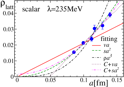
(a)	(b)

Figure 2: (Color online) The extrapolation of the scaling coefficients for the densities of the (a) scalar and axial, and (b) chirally invariant quark monopoles using various fits for $\lambda=235\,\mbox{MeV}$.

As it seen from Figures 2 the expected fit $\rho_{\mathrm{latt}}\propto a^{3}$ does not work for all types of monopoles. The corresponding quality of the fit is $\chi^{2}/d.o.f.=20$ and 82 for scalar/axial and invariant monopoles, respectively. However, the fits $\rho^{\mathrm{latt}}(a)=C+v\cdot a$ and $\rho^{\mathrm{latt}}(a)=C+s\cdot a^{2}$ give reasonable values for $\chi^{2}/d.o.f.$ (of the order of unity), while the coefficient $C$ is consistent with zero within error bars in all our fits. Setting $C=0$ we obtain that the best fits for the scalar/axial and invariant monopole densities is achieved, respectively, by the functions

$$\rho^{\mathrm{latt}}_{S,A}(a,\lambda)=s_{S,A}(\lambda)\cdot a^{2}\,,\quad\rho^{\mathrm{latt}}_{I}(a,\lambda)=v_{I}(\lambda)\cdot a\,,\qquad\lambda\neq 0\,.$$ (52)

In all these cases $\chi^{2}/d.o.f.\sim 1$. Note that the density of the scalar/axial and invariant monopoles can not be well fitted by the linear and, respectively, quadratic functions of $a$ since in these cases the quality of fits is as large as $10-20$. All discussed fits are shown in Figures 2 (a) and (b) by lines.

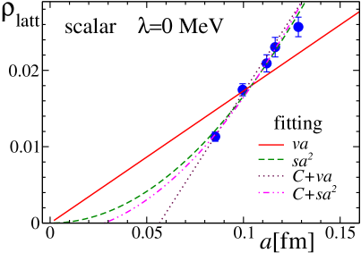
(a)	(b)

Figure 3: (Color online) The same as in Figure (2) but for the zero mode, $\lambda=0$.

The similar analysis can be performed for the zero mode, Figures 3(a) and (b). We find that the best fit functions are

$$\rho^{\mathrm{latt}}_{S,A}(a)=s_{S,A}(0)\cdot a^{2}\,,\quad\rho^{\mathrm{latt}}_{I}(a)=C_{I}(0)+s_{I}(0)\cdot a^{2}\,,\qquad\lambda=0\,,$$ (53)

with $\chi^{2}/d.o.f.\sim 1.3$ and $0.5$, respectively. The best fit parameters are

$$s_{S,A}(0)=1.66(3)\,\mbox{fm}^{2}\,,\qquad C_{I}(0)=0.094(2)\,,\quad s_{I}(0)=4.6(2)\,\mbox{fm}^{2}\,.$$ (54)

Thus, the scaling properties of the density of the invariant monopoles at $\lambda\neq 0$, Eq. (52), and at $\lambda=0$, Eq. (53), are different from each other even on the qualitative level.

We also attempted to determine the scaling behavior of the densities using the power fit of the form $C\,a^{\alpha}$, where $C$ and $\alpha$ are fitting parameters. For the non-zero modes we typically get $\alpha_{S,A}\approx 2$ and $\alpha_{I}\approx 1$ which is in agreement with the best fit function used above. For example, for the case of $\lambda=235\,\mbox{MeV}$ we get $\alpha_{S,A}=1.9(1)$ and $\alpha_{I}=1.04(7)$. The scalar/axial monopoles constructed from the of the zero Dirac mode give $\alpha_{S,A}(0)=2.1(1)$. The fit by the same dependence of the invariant monopole with $\lambda=0$ give $\alpha_{I}(0)=0.78(6)$ with higher values of $\chi^{2}/d.o.f.\approx 3$. Therefore the constant term $C_{I}\neq 0$ in the corresponding fitting function (the middle formula in Eq. (53)) is essential.

The scaling coefficients $s_{S,A}$ and $v_{I}$ obtained with the help of extrapolation (52) to the continuum limit are shown in Figures 4 (a) and (b), respectively, as functions of the Dirac eigenvalue $\lambda$.

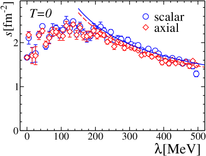
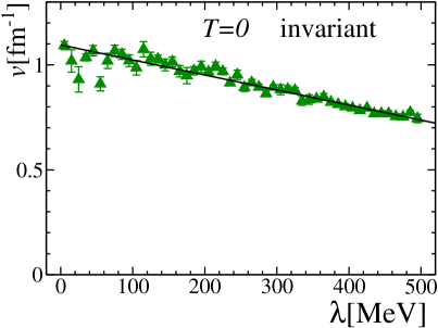
(a)	(b)

Figure 4: (Color online) The scaling coefficients for the densities of the (a) scalar and axial, and (b) chirally invariant quark monopoles. The fits by functions (55) and (56) are shown by solid and dashed lines.

The scaling coefficient $s_{S,A}(\lambda)$ of the scalar and axial monopoles has a peak around $\lambda\sim 150\,\mbox{MeV}$ while the scaling coefficient $v_{I}(\lambda)$ of the invariant mode is a monotonically decreasing function for all studied eigenvalues $\lambda$.

The behavior of the scaling coefficients $s_{S,A}$ and $v_{I}$ has some particularities. For example, we find that these scaling coefficients can be described by the formulae

$$s^{\mathrm{fit}}_{S,A}(\lambda) = l^{2}_{S,A}\cdot{\Bigl{(}\frac{\lambda}{1\,\mbox{MeV}}\Bigr{)}}^{-\gamma_{S,A}}\,,\qquad\quad\mbox{for}\quad\lambda>250\,\mbox{MeV}\,,$$ (55)

$$v^{\mathrm{fit}}_{I}(\lambda) = B_{I}\Bigl{(}1-\frac{\lambda}{\lambda_{I}}\Bigr{)}\,,\hskip 72.55452pt\mbox{for all\ }\lambda\,,$$ (56)

where the data for $s_{S,A}$ is compared with the fitting function (55) only in the region of large $\lambda$ with $\lambda>250\,\mbox{MeV}$ since in the small $\lambda$-region the behavior of this quantity is statistically unclear (there is however, a noticeable tend of $s_{S,A}$ to decrease as $\lambda\to 0$). We get (with $\chi^{2}/d.o.f.\approx 2$) the similar values for scalar and axial monopoles:

$$\gamma_{S} = 0.54(4)\,,\qquad l_{S}=0.15(2)\,\mbox{fm}\,,$$ (57)

$$\gamma_{A} = 0.44(4)\,,\qquad l_{A}=0.21(2)\,\mbox{fm}\,.$$ (58)

This result suggest that the scaling exponent $\gamma$ may be close to $1/2$ for scalar and axial types of the quark monopoles. Setting $\gamma_{S,A}=1/2$ one gets

$$\begin{array}[]{rcl}l_{S}&=&0.171(1)\,\mbox{fm}\\ \qquad l_{A}&=&0.174(1)\,\mbox{fm}\end{array}\qquad\quad\mbox{for}\quad\gamma_{S,A}=1/2\,.$$ (61)

The last fits are shown in Figure 4(a) by the solid and dashed lines for the scalar and axial monopoles, respectively.

The scaling coefficient $v_{I}$ is compared to the fitting function (56) in the whole available region of the eigenvalues $\lambda$. We get the following best fit parameters:

$$B_{I}=1.09(1)\,\mbox{fm}^{-1}\,,\qquad\lambda_{I}=1.53(4)\,\mbox{GeV}\,.$$ (62)

The corresponding fit is shown in Figure 4(b) by the solid line. One can see that the scaling of the coefficient $v_{I}$ for the invariant monopoles towards small values of the eigenvalues $\lambda$ is a smooth linear function over the whole region of studied eigenvalues $\lambda$. The $\lambda\to 0$ limit for the coefficients $s_{S,A}$ corresponding to the scalar and axial monopoles are known less accurately, as it can be seen from Figure 4(b). Summarizing, in the $\lambda\to 0$ limit we find:

$$\lim_{\lambda\to 0}s_{S,A}(\lambda)\approx 1.9(3)\,\mbox{fm}^{-1}\,,\qquad\lim_{\lambda\to 0}v_{I}(\lambda)\equiv B_{I}=1.09(1)\,\mbox{fm}^{-1}\,.$$ (63)

As it is seen from Eqs. (54), (63) the scaling coefficients $s_{S,A}$ at $\lambda=0$ for scalar and axial modes seems to coincide with the corresponding limits, $\lim_{\lambda\to 0}s_{S,A}(\lambda)\approx s_{S,A}(0)$. On the other hand, the scaling coefficient $v_{I}$ for the invariant monopole has a discontinuity at $\lambda=0$, $v_{I}(0)\neq\lim_{\lambda\to 0}v_{I}(\lambda)$, since the corresponding scaling formulae, Eqs. (52), (53), are different from each other even on the qualitative level.

III.3 Cluster structure of the monopole ensembles

The ensembles of the trajectories of the embedded monopoles can be characterized by percolation properties. As it happens in the case of the FK clusters in the Ising model, a general ensemble of the monopole trajectories consists of clusters of different types. If in the thermodynamic limit at certain physical conditions there exists a non-zero probability to find a cluster of infinite length, then the objects are said to be percolating and are often called as “condensed”. In the finite volume the role of the percolating cluster is played by a monopole cluster with the size of the order of the system volume. Using the standard terminology we call the percolating clusters as “infrared” (IR) and the short-length clusters are referred to as “ultraviolet” (UV).

In our studies we have used the following definitions of the IR and UV clusters Bornyakov:2001ux :

• The largest cluster is called the IR cluster;

• The wrapped cluster is also called the IR cluster. More precisely, for each monopole cluster $C$ we calculate the sum $S_{\mu}=\sum_{j\in C}j_{\mu}$. If this sum is nonzero then the cluster is called the IR cluster;

• Other clusters are called the UV clusters.

As an example, we show in Figures 5(a), (b) and (c) the total monopole density along with the density of the quark monopoles in the IR and the UV clusters for scalar, axial and invariant monopoles, respectively. The densities are shown at zero temperature (for $\beta=2.3493$) as functions of the eigenvalue $\lambda$.

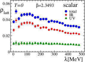
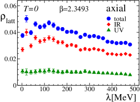
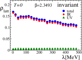
(a)	(b)	(c)

Figure 5: (Color online) The total, infrared and ultraviolet densities of the (a) scalar, (b) axial, and (c) chirally invariant embedded monopoles vs. the Dirac eigenvalue $\lambda$.

One finds that the most part of monopoles of all types belongs to the IR clusters. The IR monopole density is about 3/4 of the total monopole density in the case of the scalar and axial monopoles, while in the axially invariant case almost all (about 95%) monopoles are residing in the IR clusters. Another interesting feature of the monopole density spectrum is that the UV part of the monopole clusters is almost insensitive to the value of the Dirac eigenvalue $\lambda$. The UV density of the invariant monopoles is very small being slightly increasing function of the eigenvalue $\lambda$.

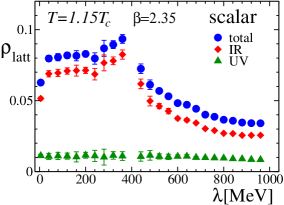
(a)	(b)	(c)

Figure 6: (Color online) The same as in Figure (5) but for the deconfinement phase at $T=1.15T_{c}$.

In order to estimate how the temperature affects the monopole densities, we show in Figure (6) the densities of the monopoles in the IR and UV clusters in the deconfinement phase at $T=1.15T_{c}$. The lattice spacing for the data shown in Figures 5 and 6 is chosen to be almost the same. One can clearly see that the basic features of the cluster structure in the deconfinement phase are similar to those in the confinement phase except for the quantitative difference: in the deconfinement phase a bigger (compared to the confinement phase) fraction of the monopoles belong to the IR cluster.

The scaling of the individual contributions (total, IR and UV) towards continuum limit is especially interesting. We found that the total and the IR parts of the lattice density of the chirally invariant monopole scale towards the continuum limit proportionally the lattice spacing $a$ for all non-zero ($\lambda>0$) modes. The UV part of the lattice density does not depend on the coupling $a$ at all, which indicates that this part is a lattice artifact. Note that the last two observations do not contradict to each other in the sense of the numerical fitting since the constant UV part is very small and is almost consistent with zero. For example, at $\lambda=235\,\mbox{MeV}$ we have $\rho^{\mathrm{latt}}_{I,UV}=0.006(5)$. Therefore the scaling of the IR and the total parts should numerically be the indistinguishable from each other, and both should follow the functional dependence (52).

As for the scalar and axial monopoles, their IR and UV clusters also scale differently. The IR part of the scalar and axial monopole densities (written in the lattice units) scales as $a^{2}$, similarly to the total density (52). As for the UV part, we have found that the scaling of the corresponding lattice density is proportional to $a$. This is drastically different from scaling of the total and infrared parts. Unlike the invariant monopole case, in the case of scalar/axial monopoles there is a substantial part of the monopoles residing in the UV clusters. Therefore the different scaling of the UV part cannot in general be neglected. Unfortunately, the accuracy of our data is such that the truncated fit (51) with two fitting parameters $v$, $s$ and with $C=\rho=0$ can not give a reliable estimate of the coefficient $v$. In order to get this coefficient with a good accuracy, we fit the data for the monopole density in the ultraviolet clusters using the linear formula

$$\rho^{\mathrm{latt}}_{\Gamma,UV}=v^{\mathrm{UV}}_{\Gamma}a\,,\qquad\Gamma=S,A\,.$$ (64)

An example of this fit is shown in Figure 7(a) and the corresponding coefficient of proportionality $v^{\mathrm{UV}}$ is plotted in Figure 7(b).

Summarizing, the scaling laws for the total, IR and UV monopole densities corresponding to non-zero Dirac eigenvalues, are

$$\begin{array}[]{llllll}\rho^{\mathrm{latt,total}}_{S,A}(a,\lambda)&=&s^{\mathrm{total}}_{S,A}(\lambda)\cdot a^{2}\,,\qquad\rho^{\mathrm{latt,total}}_{I}(a,\lambda)&=&v^{\mathrm{total}}_{I}(\lambda)\cdot a\,,\\ \rho^{\mathrm{latt,IR}}_{S,A}(a,\lambda)&=&s^{\mathrm{IR}}_{S,A}(\lambda)\cdot a^{2}\,,\qquad\rho^{\mathrm{latt,IR}}_{I}(a,\lambda)&=&v^{\mathrm{IR}}_{I}(\lambda)\cdot a\,,\\ \rho^{\mathrm{latt,UV}}_{S,A}(a,\lambda)&=&v^{\mathrm{UV}}_{S,A}(\lambda)\cdot a^{1}\,,\qquad\rho^{\mathrm{latt,UV}}_{I}(a,\lambda)&=&C^{\mathrm{UV}}_{I}(\lambda)\cdot a^{0}\,,\end{array}\qquad\lambda\neq 0\,.$$ (68)

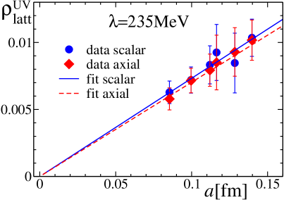
(a)	(b)

Figure 7: (Color online) (a) Example of the extrapolation of the UV fraction of the scalar and axial monopole densities at the eigenvalue $\lambda=235\,\mbox{MeV}$. The fit is done by the linear formula (64). (b) The scaling coefficient $v^{UV}$ vs. $\lambda$ for the UV part of the scalar and axial monopole densities. The quantity $v^{UV}$ is extrapolated the continuum limit.

As for the zero mode, the UV part of the density of the invariant monopoles is consistent with zero while the IR part coincide with the total monopole density within error bars. In the case of the scalar and axial monopoles both total, IR and UV parts satisfy the quadratic scaling law (53). Moreover, Eq. (68) indicates that in the continuum limit the most part of the scalar, axial, and invariant monopoles corresponding to non-zero Dirac eigenvalues ($\lambda\neq 0$) resides predominantly in UV monopole clusters. This is not the case for the exact zero mode ($\lambda=0$) which even in the continuum limit may possess both IR and UV components of the densities. So, the exact zero modes and the non-zero modes have, in fact, different embedded monopole content.

We also study the relative ratio $R$ of the monopole density in the IR clusters $\rho^{\mathrm{latt}}_{\mathrm{IR}}$ compared to the total monopole density $\rho^{\mathrm{latt}}_{\mathrm{total}}$,

$$R=\frac{\rho^{\mathrm{latt}}_{\mathrm{IR}}}{\rho^{\mathrm{latt}}_{\mathrm{total}}}\,.$$ (69)

In order to extrapolate this ratio to the continuum limit we use the linear formula:

$$R^{\mathrm{fit}}(a)=R_{0}(1-Ka)\,.$$ (70)

Here $R_{0}$ and $K$ are the fitting parameters. An example of the extrapolation and the extrapolated values of $R$ are shown in Figures 8 (a) and (b), respectively.

(a)	(b)

Figure 8: (Color online) (a) Example of extrapolation of the infrared-to-total ratios (69) corresponding to the scalar, axial, and chirally invariant embedded monopoles for the eigenvalue $\lambda=235\,\mbox{MeV}$. The fit is done by the linear formula (70). (b) The infrared-to-total ratios of the scalar, axial and invariant monopole densities extrapolated by Eq. (70) to the continuum limit vs. $\lambda$.

Note that according to Eq. (68) the formula for extrapolation (70) should contain $O(a^{2})$ corrections, which, however, can not be traced out due to limited accuracy of our data.

III.4 Discussion on scaling properties

It is interesting to speculate about the nature of the observed scaling behavior of the embedded monopole densities (51), (53), (52), (64), (68). In the zero temperature case the naive physical density, $\rho^{\mathrm{phys}}(a,\lambda)=a^{-3}\rho^{\mathrm{latt}}(a,\lambda)$, of the scalar, axial and invariant embedded monopoles diverges in the continuum limit as

$$\rho^{\mathrm{phys}}_{S,A}(a,\lambda) \sim a^{-1}\,,\qquad\rho^{\mathrm{phys}}_{I}(a,\lambda)\sim a^{-2}\,,\quad\lambda\neq 0\,,$$ (71)

$$\rho^{\mathrm{phys}}_{S,A}(a,0) \sim a^{-1}\,,\qquad\rho^{\mathrm{phys}}_{I}(a,0)\sim a^{-3}\,,\quad\lambda=0\,.$$ (72)

Let us suppose for a moment that the general quantity (51) is a density of objects of an unknown dimension, and that the individual objects are not strongly correlated in the lattice ensembles. Then, on general grounds, the terms in the formula (51) can be interpreted as follows.

If the object is of a pure lattice origin (a lattice artifact), then its lattice density should not change with the variation of the physical scale $a$. Thus, if the first term $C$ is non-zero in the continuum limit $a\to 0$, then density $\rho$ corresponds to a purely lattice object. The physics of these objects is determined by the ultraviolet cutoff $\Lambda_{\mathrm{UV}}\sim a^{-1}$ only.

Now suppose, that parameter the $C$ vanishes and the leading behavior of the lattice density is $\rho_{\mathrm{latt}}=va+\dots$ as $a\to 0$, where the coefficient $v$ is of the order of the physical QCD scale $v\sim\Lambda_{\mathrm{QCD}}$. Then the world-manifolds of the objects are the three-dimensional volumes distributed in the four-dimensional space time with the physical density $v$. The corresponding object is a membrane.

The leading scaling behavior in the form $\rho_{\mathrm{latt}}=sa^{2}+\dots$ corresponds to string-like objects, density of which is given by the quantity $s\sim\Lambda_{\mathrm{QCD}}^{2}$. Finally, if one studies pointlike objects (i.e., monopoles), which are not strongly correlated, then the scaling of their density should be $\rho_{\mathrm{latt}}=\rho a^{3}+\dots$, and the physical density of the objects should be $\rho\sim\Lambda_{\mathrm{QCD}}^{3}$.

However, these simple considerations become incorrect if the objects are (strongly) interacting with each other. As an illustrative example, it may be useful to consider currents of Abelian monopoles in an Abelian projection of pure SU(2) Yang-Mills theory. A general configuration of the gauge fields typically contain ref:clusters ; ref:vitaly two components of the monopole clusters, one of them is infrared and the other one is ultraviolet. The physical density of the infrared monopole currents is finite in the continuum limit $a\to 0$, which means that the for these monopoles the coefficients $C$, $v$ and $s$ in Eq. (51) are zero. On the other hand, the ultraviolet component of the Abelian monopole density diverges as $a^{-1}$ in physical units. One can understand this scaling as a consequence of a strong correlation between segments of the monopole loops at the scale of the lattice spacing $a$ because a typical UV monopole cluster is, in fact, a loop of the length of a few lattice spacings. One can equivalently say that the monopole clusters are short-ranged dipoles. The nature of this strong correlation is of a purely lattice origin as the recent data shows ref:vitaly . Indeed, it was found in Ref. ref:vitaly that the density of the UV monopoles strongly depends on the UV-properties of the gluon action. The density of the IR monopole clusters are also sensitive to the lattice details of the gluon action, since the artificial UV monopoles may randomly connect to the physical IR clusters and be counted by a lattice algorithm as a part of the physical IR cluster.

Thus the $a^{-1}$ and $a^{-2}$ scaling of the physical densities of the scalar/axial and, respectively, invariant embedded monopoles may be a result of the lattice procedure(s) which may be sensitive to the UV-scale. On the other hand one can not exclude a possibility that the embedded QCD monopoles may be strongly correlated with objects which have surface-like and $3D$ volume-like world trajectories. This property is supported by the observation Gubarev:2005jm that the low-lying fermion modes show unusual localization properties being sensitive both to the physical scale $\Lambda_{\mathrm{QCD}}$ and to the ultraviolet cut-off, $a^{-1}$. If this suggestion is correct, then the scaling of the “slave” monopoles may manifest the scaling of the “master” objects. In this case the scalar/axial and invariant monopoles should be correlated with (or, as one can also say, “lie on”) strings and membranes, respectively. In this paper we are not performing a detailed scaling analysis of the monopole clusters concentrating on simplest properties only. A review of the lattice data on many-dimensional vacuum objects in four-dimensional Yang-Mills theory can be found in Ref. ref:lower:dimensional:Zakharov .

Finally, let us note that the embedded monopoles are likely not lattice artifacts because their densities scale as non-zero powers of the lattice spacing $a$. Still, the effect of the lattice artifacts on the density may be noticeable since the gauge fields are not improved at all contrary to the Dirac eigenmodes which are greatly improved by using the overlap fermions.

IV Embedded monopoles and fermion spectral density

One of the most essential characteristics of the fermion modes in the gauge theory is the fermion spectral density $\rho_{F}$ which is formally defined as the expectation value

$$\rho_{F}(\lambda)=\frac{1}{V}\langle\sum_{\bar{\lambda}}\delta(\lambda-\bar{\lambda})\rangle\,,$$ (73)

where the sum goes over all Dirac eigenvalues $\bar{\lambda}=\bar{\lambda}(A)$ corresponding to gauge fields configurations $A$ which enter the partition function. The low-lying part of the fermion spectrum is important for the chiral symmetry breaking due to the Banks-Casher formula ref:Banks:Casher ,

$$\langle\bar{\psi}\psi\rangle=-\lim_{\lambda\to 0}\pi\rho_{F}(\lambda)\,,$$ (74)

which relates the chiral condensate $\langle\bar{\psi}\psi\rangle$ with the spectral density.

Examples of the spectral density $\rho_{F}$ as functions of $\lambda$ are shown in Fig. 9 for the confinement ($T=0$, $\beta=2.3493$) and for the deconfinement ($T=1.15T_{c}$, $\beta=2.35$) phases. In the zero temperature (confinement) case the spectrum is a gradually increasing function of the eigenvalue $\lambda$, and the low-energy part of the spectrum has a finite $\lambda\to 0$ limit. In the deconfinement phase the low-energy part of the spectrum is suppressed compared to the confinement phase but is, however, non-zero. This feature as well as the peak of the spectral density at $\lambda=0$ may be an artifact related to an effect of the finite volume. We expect that in the limit of an infinite volume the spectrum above the deconfinement temperature should vanish below some critical value $\lambda_{c}(T)$. This property could imply vanishing of the chiral condensate (74) in the deconfinement phase, $\langle\bar{\psi}\psi\rangle(T>T_{c})=0$. In our case the critical value is $\lambda_{c}(T=1.15\,T_{c})\approx 400\,\mbox{MeV}$.

Figure 9: (Color online) Spectral fermion density in the confinement ($T=0$, $\beta=2.3493$) and in the deconfinement ($T=1.15T_{c}$, $\beta=2.35$) phases.

The embedded QCD monopoles are suggested ref:embedded:QCD to be agents the chiral symmetry restoration, since in the cores of these monopoles the chiral invariance should be unbroken. According to the proposed scenario, one can expect that at low Dirac eigenvalues – which are relevant to the chiral symmetry breaking due to the Banks-Casher relation (74) – the density of the embedded monopoles should be high in the chirally invariant (high temperature) phase and the density should be relatively low in the chirally broken (low temperature) phase. Thus suggestion implies, in turn, that the density of the embedded monopoles should be anti-correlated with the fermion spectral function: the lower value of the spectral function the higher monopole density is expected to be. In particular, in the high temperature phase the vanishing spectral function at $\lambda<\lambda_{c}$ implies the high density of the quark monopoles for $\lambda<\lambda_{c}$, and vice versa.

The anti-correlation of the quark monopole density and the fermion spectral function is indeed observed in deconfinement phase as it is shown in Figure 1(d). Indeed, as one can see from comparison of Figure 1(d) and the $T=1.15T_{c}$ spectral function shown in Figure 9, at high $\lambda$ the fermion spectral function is high corresponding to low embedded monopole density, while at low $\lambda$ the fermion spectral density is suppressed in accordance with the observed large valued of the monopole density.

In the confinement case the qualitative relation between the spectral density and the embedded monopole density is true as well according to Figures 1(a),(b),(c) and Figure 9: the fermion spectrum is an increasing function of the Dirac eigenvalue $\lambda$ while the monopole densities are generally decreasing function of $\lambda$.

V Excess of gluon action on quark monopoles

If the embedded QCD monopoles are physical objects then we would expect that these objects are locally correlated with the action density and, presumably, with the topological charge. Following Refs. ref:Bakker ; ref:Monopole:Structure we calculate numerically the excess of the SU(2) gauge action at the position of the embedded monopole currents $j_{x,\mu}$,

$$f_{S}=\frac{\langle|j_{x,\mu}|\,S_{c_{x,\mu}}\rangle-6\langle|j_{x,\mu}|\rangle\langle S_{P}\rangle}{\langle|j_{x,\mu}|\rangle}\,,\,,$$ (75)

where $S_{c}$ is the sum over the elementary plaquette actions,

$$S_{c}=\sum_{P\in\partial c}S_{P}\,,\qquad S_{P}=1-\frac{1}{2}\,{\mathrm{Tr}}U_{P}\,,$$

belonging to the six faces $P$ of the cubes $c\equiv c_{x,\mu}$ with non-zero monopole charge, $j_{x,\mu}\neq 0$. Here $U_{P}$ is the $SU(2)$ plaquette constructed from the lattice links $U_{x\mu}$ in the standard way $U_{P_{x,\mu\nu}}=U_{x\mu}U_{x+\hat{\mu},\nu}U^{\dagger}_{x+\hat{\nu},\mu}U^{\dagger}_{x\nu}$. The second term in Eq. (75) subtracts the vacuum average of the action from the value of the gluon action at the monopole.

Equation (75) can be understood as the (average) excess of the Yang-Mills action calculated at the (average) distance $r=a/2$ from the center of the monopole. In fact, in any given lattice configuration the position of the monopole center can not be determined exactly within the lattice the cube possessing a nonzero monopole charge. However on average the monopole center is located as the cube center which resides at the distance $a/2$ from any face (plaquette) of the cube. It is worth noticing that Eq. (75) defines the excess of the chromomagnetic part of the action since by construction the action around the monopole is calculated on the plaquettes $P$ perpendicular to the corresponding link $l=\{x,\mu\}$ of the monopole trajectory.

In the naive continuum limit the elementary plaquette, say $P_{x,12}$, is expanded in powers of the lattice spacing as follows

$$S_{P_{x,12}}(a)=a^{4}\,\frac{g^{2}}{8}\,{\bigl{[}F^{a}_{12}(x)\bigr{]}}^{2}+O(a^{6})$$ (76)

where $g$ is the (bare) coupling and $U_{x\mu}=e^{iagA_{\mu}(x+\hat{\mu}/2)}$. Thus the excess of the action (75) can be written as (we omit $O(a^{6})$ corrections starting from here)

$$f_{S}(a) = a^{4}\,\frac{\pi}{2}\,\mathcal{B}_{\mathrm{mon}}(a/2)\,,$$ (77)

where

$$\mathcal{B}_{\mathrm{mon}}(a/2) = {\bigl{\langle}\alpha_{s}\,{({\mathbf{B}}^{c})}^{2}\,\bigr{\rangle}}_{\mathrm{mon}}{\Bigr{|}}_{r=a/2}-{\bigl{\langle}\alpha_{s}\,{({\mathbf{B}}^{c})}^{2}\,\bigr{\rangle}}\,,$$ (78)

is the excess of the chromomagnetic condensate at the distance $r=a/2$ from the quark monopole and $\alpha_{s}=g^{2}/(4\pi)$. The chromomagnetic field at the segment of the monopole current $j_{\nu}$ is defined as $B^{c}_{\mu}(j_{\nu})=-\epsilon_{\mu\nu\alpha\beta}F^{c}_{\alpha\beta}/2$. This definition reduces to the standard one for a static ($\nu=4$) monopole: $B^{c}_{i}=\epsilon_{ijk}F^{c}_{jk}/2$ with $i,j,k=1,2,3$. In the Euclidean space-time at zero temperature the chromomagnetic and the standard gluon condensates are related as ${\bigl{\langle}\alpha_{s}\,{({\mathbf{B}}^{c})}^{2}\bigr{\rangle}}={\bigl{\langle}\alpha_{s}\,{(F^{c}_{\mu\nu})}^{2}\,\bigr{\rangle}}/2$.

Before proceeding with analysis of the numerical data it would be instructing to discuss the expected behavior of the chromomagnetic fields inside the embedded monopoles at least on a qualitative level. In Ref. ref:embedded:QCD the embedded QCD monopole is associated with the Nambu monopole in the Electroweak model. The Nambu monopole is essentially the ’t Hooft-Polyakov ref:thooft ; ref:polyakov (HP) monopole configuration embedded into the EW model. Therefore one naively can expect that the behavior of the chromomagnetic fields inside the embedded monopole in QCD is qualitatively similar to that of the HP monopole in the Georgi-Glashow model.

As an illustrative example let us consider the Bogomol’ny-Prassad-Sommerfeld (BPS) limit ref:BPS of the Georgi-Glashow model,

$${\cal L}_{\mathrm{GG}}=\frac{1}{4}(F^{a}_{\mu\nu})^{2}+\frac{1}{2}\left(D^{\mathrm{ad}}_{\mu}\Phi\right)^{2}+\frac{\lambda}{4}\left((\Phi^{a})^{2}-\eta^{2}\right)^{2}\,.$$ (79)

This model describes the dynamics of the $SU(2)$ gauge field $A^{a}_{\mu}$ interacting with the triplet (adjoint) Higgs field $\Phi^{a}$, $a=1,2,3$. The adjoint covariant derivative is given in Eq. (15). The scalar coupling $\lambda$ describes self-interaction of the Higgs field. The condensate of the Higgs field is $|\langle\vec{\Phi}\rangle|=\eta$. The masses of the gauge and Higgs fields in the Georgi-Glashow model are, respectively, $m_{A}=g\,v$ and $m_{\Phi}=\sqrt{2\lambda}\,\eta$.

The BPS limit is defined by the condition $\lambda=0$, which sets the mass of the Higgs particle to zero, $m_{\Phi}=0$. Due to the absence of the quartic Higgs self-interaction the classical static ’t Hooft-Polyakov solution can be found explicitly ref:BPS :

$$\Phi^{a}=\frac{r^{a}}{g\,r^{2}}H(\eta g\,r)\,,\qquad A^{a}_{i}=\epsilon_{aij}\frac{r^{j}}{g\,r^{2}}[1-K(\eta g\,r)]\,,\qquad A^{a}_{0}=0\,,$$ (80)

where

$$K(\xi)=\frac{\xi}{\sinh\xi}\,,\qquad H(\xi)=\xi\coth\xi-1\,,$$ (81)

The chromoelectric field of the HP monopole is zero, $F^{a}_{0i}\equiv 0$, and the chromomagnetic field $B^{c}_{i}=\epsilon_{ijk}F^{c}_{jk}/2$, is:

$$B^{c}_{i}=\frac{r^{c}\,r^{i}}{g\,r^{4}}\Bigl{(}1-K^{2}-HK\Bigr{)}+\frac{\delta^{ci}}{g\,r^{2}}\,HK\,,$$ (82)

The corresponding “condensate” of the chromomagnetic field tends to a finite value in the monopole center, $r\to 0$:

$$\mathcal{B}_{\mathrm{HP}}(r) \equiv \frac{g^{2}}{4\pi}{[{\mathbf{B}}^{c}(r)]}^{2}=\frac{1}{4\pi r^{4}}\,\Bigl{[}\Bigl{(}1-K^{2}(\eta g\,r)\Bigr{)}^{2}+2H^{2}(\eta g\,r)\,K^{2}(\eta g\,r)\Bigr{]}\,,$$ (83)

$$\mathcal{B}_{\mathrm{HP}}(r) = \mathcal{B}_{\mathrm{HP}}^{(0)}\cdot\Bigl{[}1+O((\eta gr)^{2})\Bigr{]}\,,\qquad\mathcal{B}_{\mathrm{HP}}^{(0)}=\frac{\eta^{4}g^{4}}{12\,\pi}\qquad\mbox{for}\quad r\to 0\,.$$ (84)

Let us take for a moment this illustrative example of the hedgehog configuration seriously. The QCD counterpart of the field $\Phi^{a}$ is an octet quark-antiquark composite field $\xi^{a}$. We do not expect the presence of the octet condensates $\langle\xi^{a}\rangle$ in vacuum of the Yang-Mills theory because such a condensate must inevitably break the color symmetry (see, however, a discussion in Ref. ref:wetterich ). On the other hand one may expect ref:embedded:QCD that the non-perturbative color-invariant four-quark condensates ref:four:quark of the form $\langle(\xi^{a})^{2}\rangle$ should stabilize the hedgehog-like configurations made of the composite “Higgs” field $\xi^{a}$ in the confinement phase.

One can expect that the value of the condensate $\eta$ in Eqs. (83), (84) should be of the order of a typical dimensional quantity describing the chiral condensate, $\eta\sim|\langle\bar{\psi}\psi\rangle|^{1/3}\sim 0.2\dots 0.3\,\mbox{GeV}$, which, in turn, is of the order of the QCD scale parameter $\Lambda_{\mathrm{QCD}}$. One can think of $\eta$ as of the condensate outside the core. The gauge coupling $g$ can be associated with the QCD running coupling. Then Eq. (84) predicts that the chromomagnetic field inside the embedded monopole should be “soft”,

$$\mathcal{B}_{\mathrm{mon}}(r)\sim g^{4}(r\Lambda_{\mathrm{QCD}})\cdot\Lambda^{4}_{\mathrm{QCD}}\,.$$

In particular, this relation implies the absence of the hard ultraviolet divergences of the energy density inside the monopole cores contrary to the case of the Abelian (Dirac) monopoles ref:fine:tuning ; ref:Monopole:Structure .

We perform the fit of the numerical data for the correlation function (75) by

$$f^{\mathrm{fit,HP}}_{S}=2\,\Bigl{[}\Bigl{(}1-K^{2}(x)\Bigr{)}^{2}+2K^{2}(x)H^{2}(x)\Bigr{]}\,,\quad x=g(\Lambda_{\mathrm{HP}}\,a/2)\cdot\eta a/2\,,$$ (85)

which can be obtained from Eqs. (77), (83) by identification $r=a/2$. The function $K$ is given in Eq.(81), and instead of the Georgi-Glashow coupling $g$ we take the one-loop running coupling constant of the SU(2) Yang–Mills theory,

$$g^{-2}(\Lambda a)=\frac{11}{12\pi^{2}}\log\frac{1}{\Lambda a}\,.$$ (86)

The fitting parameters are the HP scale parameter $\Lambda_{\mathrm{HP}}$ and the “condensate” parameter $\eta$.

(a)	(b)

Figure 10: (Color online) The excess of the chromomagnetic action (75) at (a) the scalar and (b) the chirally invariant monopoles at $\lambda=0$ and $\lambda=235\,\mbox{MeV}$. The solid and the dotted lines refer to the fits Eq. (85) and (87), respectively.

Examples of the correlation function $f_{S}$ at $\lambda=0$ and $\lambda=235\,\mbox{MeV}$ are shown in Figures 10(a) and (b) for scalar and chirally invariant monopoles, respectively. The excess of the chromomagnetic energy for the scalar and axial monopoles coincide with each other within error bars. The examples of the fits of the excess energy by the function (85) are shown by the solid lines. One can see that the fitting formula (81), (85), (86) – which is resembling the ’t Hooft-Polyakov monopole configuration in the Bogomol’ny limit (81), (80), (81) – emulates our numerical data relatively well. The fitting is better near the continuum limit, $a\to 0$. However at relatively large distances, $a\gtrsim 0.13\,\mbox{fm}$, the data and the best fit function show some noticeable difference which makes $\chi^{2}/d.o.f\sim 3\dots 5$ for these fits.

The best fit parameters $\Lambda_{\mathrm{HP}}$ and $\eta$ obtained in our fits by the function (85) come with relatively large errors. For example, for scalar monopoles at $\lambda=0$ we have $\Lambda_{\mathrm{HP}}=17(26)\,\mbox{MeV}$ and $\eta=136(14)\,\mbox{MeV}$, while at $\lambda=235\,\mbox{MeV}$ we get $\Lambda_{\mathrm{HP}}=28(31)\,\mbox{MeV}$ and $\eta=98(12)\,\mbox{MeV}$. The corresponding numbers for the invariant monopoles are: in the $\lambda=0$ case we obtain $\Lambda_{\mathrm{HP}}=30(36)\,\mbox{MeV}$ and $\eta=72(17)\,\mbox{MeV}$, while for $\lambda=235\,\mbox{MeV}$ we get $\Lambda_{\mathrm{HP}}=24(20)\,\mbox{MeV}$ and $\eta=75(10)\,\mbox{MeV}$. Thus the values of the parameter $\Lambda_{\mathrm{HP}}$ can not be defined well due to quite weak dependence of the logarithm function (86) on the value of its argument. Moreover, the value of $\Lambda_{\mathrm{HP}}$ is very small what makes $g\sim 1$ in all our fits. On the other hand the fit quantitatively confirms that the values for the “condensate” $\eta$ is of the order of the QCD scale, $\eta\sim\Lambda_{\mathrm{QCD}}$. The effective size of the “HP monopole” core, $1/m_{A}=1/(g\eta)$, can be estimated to be of the order of 1 fm for all values of $\lambda$. Since this value is unrealistically large we conclude that the fact that the HP fitting formula (85) works relatively well is only a manifestation of the “softness” of the gluonic action inside the core of the monopole. Quantum corrections to the HP monopole fields may be important.

In order to get prescription-independent result on the scaling of the average action excess we fit the available data by the power-like fitting function

$$f^{\mathrm{fit,power}}_{S}(a)={\left(a/h\right)}^{4+\delta}\,,$$ (87)

where the scale $h$ and the “anomalous” exponent $\delta$ are the fitting parameters. If the action density is independent on the distance to the monopole center (or, in other words, if the core of the embedded monopoles is structure-less) then we would naively expect the vanishing anomalous exponent, $\delta=0$. If $\delta\neq 0$ then one can expect some structure of the monopole core.

The example of the fits (87) at $\lambda=0$ and $\lambda=235\,\mbox{MeV}$ are shown in Figures 10(a) and (b) by the dotted lines. As one can see from these Figures, the HP monopole fit (85) and the simple power fit (87) are practically indistinguishable from each other. Note that both fits are two-parametric ones.

(a)	(b)

Figure 11: (Color online) The best fit parameters (a) $h$ and (b) $\delta$ of the fit function (87) vs. the Dirac eigenvalue $\lambda$ for the scalar, axial and chirally invariant embedded monopoles.

The best fit parameters for the power function (87) are shown in Figures 11(a) and (b) as functions of $\lambda$ for all studied types of the quark monopoles. We find that both $h$ and $\delta$ parameters are almost independent on the Dirac eigenvalue $\lambda$. Moreover, these parameters for different types of the quark monopole are quite close to each other. This result suggests that the gluonic structure of the embedded monopoles seems to be independent on the value of $\lambda$. The typical values of the fitting parameters are concentrating around central values $h_{S,A}\approx 1.6\,\mbox{fm}$, $h_{I}\approx 2\,\mbox{fm}$ and $\delta_{S,A,I}\approx 0.7$ with, however, relatively large error bars.

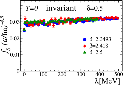
(a)	(b)

Figure 12: (Color online) The local excess (75) of the Yang-Mills action at the position of the (a) scalar and (b) invariant monopoles, scaled by the power function, $f_{S}(a)\,a^{-(4+\delta)}$, with the anomalous scaling exponent $\delta=1/2$. The three values of the lattice coupling $\beta$ are shown.

In order to get an impression on the quality of the power-like scaling (87) we plot in Figures 12 (a) and (b) the scaling function $f_{S}$ multiplied by the factor $a^{-(4+\delta)}$ with $\delta=1/2$ for the three different values of the lattice coupling constant $\beta$. Figures 12(a) and (b) clearly show that the quantity $f_{S}(a)\,a^{-4.5}$ is independent of the lattice spacing $a$ for the embedded monopoles of all three types. Since the fits of by the power (87) and the HP-inspired (85) functions are practically indistinguishable at our data sets (as one can see from examples plotted in Figures 10(a) and (b)), the scaling of our data with the HP-type energy excess (85) should be as remarkable as it is plotted in Figures (12) for the power-profile excess (87).

It is interesting to point out that despite noticeably different scaling (52) of the scalar/axial and chirally invariant monopole densities towards continuum limit, the excess of the action density at the positions of these monopoles scales essentially in the same way.

Since the monopole cores are “soft” we do not expect a fine-tuning ref:fine:tuning between the energy and entropy of these monopoles (at least, in the studied case of the pure SU(2) Yang-Mills theory). On the other hand, the embedded monopoles does not scale as particle like objects, therefore the investigation of the energy-entropy balance in the case of the embedded monopoles in the quenched case may be a complicated issue.

A cautionary remark here is that the monopoles are detected with the help of the operators (20) which implicitly depend on the lattice spacing $a$. If the monopole has a core-like structure of the size of the lattice spacing then the ability of the numerical procedure to “detect” a lattice monopole within the lattice cube should be very sensitive to the size of the “detector” (i.e. to the lattice spacing). In order to get physically reliable results on the monopole density and the monopole correlations one should probably study the scaling of the extended (blocked) monopoles ref:Extended:Monopoles .

Summarizing, both scalar, axial and invariant embedded monopoles are locally correlated with the magnetic part of the gluonic action. The excess of the action at fixed lattice spacing $a$ (or, equivalently, at fixed $\beta$) is a slowly increasing function of the Dirac eigenvalue $\lambda$. The average action excess on the scalar and axial monopoles coincide with each other and is approximately two times higher than the excess of the action on the invariant monopoles. The positive value of $f_{S}(a)$ indicates that the action density near the monopole is increased compared to the average density. Thus the embedded monopole has a chromomagnetic core. On the other hand, the positive value of the anomalous scaling exponent $\delta$ indicates that the excess of the chromomagnetic action decreases as one approaches the center of the monopole core. Concretely, the chromomagnetic condensate vanishes in the center of the embedded monopoles as

$$\mathcal{B}_{\mathrm{mon}}(r)\sim r^{\delta}\,,\qquad\delta\sim 0.5\dots 1\,.$$ (88)

Thus, the embedded monopoles possess “chromomagnetically” empty cores.

VI Conclusions

We study basic properties of the embedded QCD monopoles in the pure SU(2) Yang-Mills theory. The monopole trajectories are found with the help of the low-lying eigenmodes of the overlap Dirac operator. These modes are then treated as $c$-valued quark fields, the behavior of which emulates the basic chiral properties of the QCD vacuum.

The embedded monopoles are explicitly gauge-invariant, and the magnetic charge of the monopole is quantized and conserved. Basically, the embedded QCD monopoles are the gauge-invariant hedgehogs in the quark-antiquark condensates (therefore we also call these monopoles as “quark monopoles”).

We give the lattice definitions of the embedded monopoles of scalar, axial and chirally invariant types. We find that the scaling of the scalar and axial monopole densities towards the continuum limit is the same as the scaling of the string-like objects. The scaling of the chirally invariant monopoles corresponds to the one of the membrane-like objects. This result may indicate that the monopole trajectories are correlated with higher-dimensional (string-like and membrane-like) objects in the $SU(2)$ Yang-Mills theory. The “scalar/axial string”, for example, may be a border of the “chirally invariant membrane”. We also observe a difference in the scaling properties of the monopoles corresponding to the non-zero and to the zero Dirac eigenvalues.

The embedded QCD monopoles were suggested ref:embedded:QCD to be related to the restoration of the chiral symmetry in the high-temperature phase since their cores should contain the chirally symmetric vacuum. Our numerical study supports this suggestion since the monopole density is anti-correlated with the density of the Dirac eigenmodes. In particular, at low Dirac eigenvalues – which are relevant to the chiral symmetry breaking due to the Banks-Casher relation – the density of the embedded monopoles is high in the chirally invariant (high temperature) phase and is relatively low in the chirally broken (low temperature) phase.

We find that the embedded monopoles have gluonic cores, which are more pronounced for the chirally invariant monopoles compared to the scalar/axial monopoles. On average, the chromomagnetic energy near the monopole trajectories is higher compared to the chromomagnetic energy far from the monopole core. However, our scaling analysis suggests that at the very center of the embedded QCD monopole, the excess of the chromomagnetic energy reduces back to the vacuum expectation value. Therefore a typical monopole core is a bump in the chromomagnetic energy which takes its maximum value at a certain finite distance from the monopole center. Outside this bump – towards the monopole center and/or far from the monopole core – the energy density diminishes to its vacuum expectation value. This structure is similar to the structure of the ‘t Hooft-Polyakov monopoles if one attributes to the asymptotic freedom the suppression of the chromomagnetic gluon condensate in the monopole center.

Finally, we would like to remark that one can not exclude a possibility that the properties of the embedded monopoles in the full QCD may drastically be different from the quenched case. On the other hand the quenched theory mimics chiral instability of the full QCD to develop a chiral condensate at low temperatures. Therefore our results support the suggestion that the quark monopoles are tightly related to the chiral symmetry restoration also in the case of the real QCD.

Note added

When numerical calculations were completed we became aware that a similar procedure has been applied earlier in $SU(3)$ lattice gauge theory ref:Gerrit .

Appendix A Details of numerical simulations

We simulate numerically the SU(2) lattice gauge theory with the standard Wilson action, $S_{P}=\beta(1-(1/2){\mathrm{Tr}}\,U_{P})$, where $\beta$ is the SU(2) gauge coupling and $U_{P}$ is the SU(2) plaquette variable constructed from the lattice link fields $U(x,\mu)$. We used various values of $\beta$ at different lattice sizes to check the scaling of the numerically calculated observables towards the continuum limit. The parameters of the numerical simulations are given in Table 1.

$T=0$
$\beta$	$a$[fm]	$L_{s}$	$L_{t}$	$N_{conf}$	$\beta$	$a$[fm]	$L_{s}$	$L_{t}$	$N_{conf}$	$\beta$	$a$[fm]	$L_{s}$	$L_{t}$	$N_{conf}$
2.3493	0.1397(15)	10	10	300	2.3772	0.1284(15)	10	14	90	2.4071	0.1164(15)	12	12	180
2.4180	0.1120(15)	12	14	150	2.4500	0.0996(22)	14	14	200	2.5000	0.0854(4)	16	18	200
$T=1.15T_{c}$
					2.3500	0.1394(8)	16	4	200

Table 1: (Color online) Parameters of the simulations.

The first 6 points in Table 1 correspond to the zero temperature (confinement) phase. The lattice geometries and values of the lattice coupling $\beta$ are tuned in order to keep the lattice volume constant, $V=3.8\,\mbox{fm}^{4}$. The point with $\beta=3.5$ has a little bigger volume, $V=3.92\,\mbox{fm}^{4}$.

In order to have an impression about the behavior of the quark monopoles in the high temperature phase we study one point at asymmetric lattice $16^{3}\times 4$. At these lattices the system is just above the finite temperature critical point with $T=1.15\,T_{c}$.

In order to define the quark monopoles one may use eigenmodes of the Dirac operator in the background of the gauge field. In our lattice simulations we use the overlap fermions which possess an exact chiral symmetry, enjoy automatic $O(a)$ improvement, and are not defaced by exceptional configurations ref:overlap . The overlap Dirac operator is

$$D=\frac{\rho}{a}\left(1+D_{w}/\sqrt{D_{w}D_{w}^{\dagger}}\right)=\frac{\rho}{a}(1+\gamma_{5}\,{\mathrm{sign}}(H)),\ \ \ H=\gamma_{5}D_{w}\,,$$ (89)

where $D_{w}$ is the Wilson Dirac operator with negative mass term and $H$ is hermitian Wilson Dirac operator. The value of $\rho$ parameter is equal to $1.4$. We have used the minimax polynomial approximation to compute the sign function. In order to improve the accuracy and performance about one hundred lowest eigenmodes of $H$ were projected out. The eigenvalues of $D$, which lies on the circle in the complex plain, were stereographically projected onto the imaginary axis in order to relate them with continuous eigenvalues of the Dirac operator.

References

- (1) K. Rajagopal, F. Wilczek, in At the Frontier of Particle Physics, edited by M. Shifman (World Scientific, Singapore, 2001), Vol. 3, p. 2061 [hep-ph/0011333].
- (2) S. D. Katz, Nucl. Phys. Proc. Suppl. 129, 60 (2004); Z. Fodor, S. D. Katz, JHEP 0404, 050 (2004).
- (3) M. N. Chernodub, Phys. Rev. Lett. 95, 252002 (2005).
- (4) For a review, see A. Achucarro, T. Vachaspati, Phys. Rept. 327 (2000) 347.
- (5) Y. Nambu, Nucl. Phys. B 130, 505 (1977).
- (6) N. S. Manton, Phys. Rev. D 28, 2019 (1983).
- (7) T. Vachaspati, in Electroweak Physics and the Early Universe, J. C. Romão and F. Freire (Eds.), Plenum, New York, 1995, p. 171, hep-ph/9405286.
- (8) M. N. Chernodub, JETP Lett. 66, 605 (1997).
- (9) M. N. Chernodub, F. V. Gubarev, E. M. Ilgenfritz, A. Schiller, Phys. Lett. B 434, 83 (1998).
- (10) M. N. Chernodub, F. V. Gubarev, E. M. Ilgenfritz, A. Schiller, Phys. Lett. B 443, 244 (1998).
- (11) M. Reuter, C. Wetterich, Nucl. Phys. B 408, 91 (1993); K. Kajantie, M. Laine, K. Rummukainen, M. Shaposhnikov, Phys. Rev. Lett. 77, 2887 (1996); Nucl. Phys. B 466, 189 (1996); M. Gurtler, E. M. Ilgenfritz, A. Schiller, Phys. Rev. D 56, 3888 (1997).
- (12) J. Kertész, Physica A161, 58 (1989).
- (13) C. M. Fortuin, P. W. Kasteleyn, Physica 57, 536 (1972).
- (14) M. Baig, J. Clua, Phys. Rev. D 57, 3902 (1998); S. Wenzel, E. Bittner, W. Janke, A. M. J. Schakel, A. Schiller, Phys. Rev. Lett. 95, 051601 (2005).
- (15) G. Baym, Physica 96A, 131 (1979); T. Celik, F. Karsch, H. Satz, Phys. Lett. B 97, 128 (1980); H. Satz, Rept. Prog. Phys. 63, 1511 (2000);
- (16) For a review, see H. Satz, Nucl. Phys. A 681, 3 (2001).
- (17) R. Bertle, M. Faber, J. Greensite, S. Olejnik, Phys. Rev. D 69, 014007 (2004).
- (18) G. ’t Hooft, Nucl. Phys. B 79, 276 (1974).
- (19) M. N. Chernodub, F. V. Gubarev, E. M. Ilgenfritz, Phys. Lett. B 424, 106 (1998).
- (20) Yakov M. Shnir, “Magnetic Monopoles” (Springer, 2005); Phys. Scr. 69, 15 (2004); hep-th/0508210.
- (21) M. N. Chernodub (unpublished).
- (22) E. J. Weinberg, Phys. Rev. D 20, 936 (1979); Nucl. Phys. B 167, 500 (1980); ibid., 203, 445 (1982).
- (23) K. Fujikawa, Phys. Rev. Lett. 44, 1733 (1980); Phys. Rev. D 21, 2848 (1980).
- (24) T. A. DeGrand, D. Toussaint, Phys. Rev. D22, 2478 (1980).
- (25) V. Bornyakov, M. Muller-Preussker, Nucl. Phys. Proc. Suppl. 106, 646 (2002); V. G. Bornyakov, P. Y. Boyko, M. I. Polikarpov, V. I. Zakharov, Nucl. Phys. B 672, 222 (2003).
- (26) S. i. Kitahara, Y. Matsubara, T. Suzuki, Prog. Theor. Phys. 93, 1 (1995); A. Hart, M. Teper, Phys. Rev. D 58, 014504 (1998); M. N. Chernodub, V. I. Zakharov, Nucl. Phys. B 669, 233 (2003).
- (27) V. G. Bornyakov, E. M. Ilgenfritz, M. Muller-Preussker, Phys. Rev. D 72, 054511 (2005).
- (28) V. I. Zakharov, Phys. Atom. Nucl. 68, 573 (2005).
- (29) C. Aubin et al. [MILC Collaboration], Nucl. Phys. Proc. Suppl. 140, 626 (2005); F. V. Gubarev, S. M. Morozov, M. I. Polikarpov, V. I. Zakharov, JETP Lett. 82, 343 (2005); Y. Koma, E. M. Ilgenfritz, K. Koller, G. Schierholz, T. Streuer, V. Weinberg, PoS LAT2005, 300 (2005); C. Bernard et al., PoS LAT2005, 299 (2005); E. M. Ilgenfritz, K. Koller, Y. Koma, G. Schierholz, T. Streuer, V. Weinberg, “Probing the topological structure of the QCD vacuum with overlap fermions”, hep-lat/0512005; A. V. Kovalenko, S. M. Morozov, M. I. Polikarpov, V. I. Zakharov, “On topological properties of vacuum defects in lattice Yang-Mills theories”, hep-lat/0512036.
- (30) T. Banks, A. Casher, Nucl. Phys. B 169, 103 (1980).
- (31) B. L. G. Bakker, M. N. Chernodub, M. I. Polikarpov, Phys. Rev. Lett. 80, 30 (1998).
- (32) V. G. Bornyakov et al., Phys. Lett. B 537, 291 (2002); V. A. Belavin, M. I. Polikarpov, A. I. Veselov, JETP Lett. 74, 453 (2001).
- (33) A. M. Polyakov, JETP Lett. 20, 194 (1974).
- (34) E. B. Bogomolny, Sov. J. Nucl. Phys. 24, 449 (1976); M. K. Prasad, C. M. Sommerfield, Phys. Rev. Lett. 35, 760 (1975); for a review see Yakov M. Shnir, “Magnetic Monopoles” (Springer, 2005).
- (35) C. Wetterich, Phys. Lett. B 462, 164 (1999); Phys. Rev. D 64, 036003 (2001); J. Berges, C. Wetterich, Phys. Lett. B 512, 85 (2001), where the idea of the spontaneous breaking of color by quark condensates is discussed.
- (36) M. B. Johnson, L. S. Kisslinger, Phys. Rev. D 61, 074014 (2000).
- (37) V. I. Zakharov, “Fine tuning in lattice SU(2) gluodynamics vs continuum-theory constraints”, hep-ph/0306262; “Confining fields in lattice SU(2)” hep-ph/0312210.
- (38) T. L. Ivanenko, A. V. Pochinsky, M. I. Polikarpov, Phys. Lett. B 252, 631 (1990); H. Shiba, T. Suzuki, Phys. Lett. B 351, 519 (1995); S. Kato, N. Nakamura, T. Suzuki, S. Kitahara, Nucl. Phys. B 520, 323 (1998); M. N. Chernodub et al., Phys. Rev. D 62, 094506 (2000).
- (39) V. G. Bornyakov, G. Schierholz, T. Streuer, unpublished (2005).
- (40) H. Neuberger, Phys. Lett. B 417, 141 (1998); ibid. 427, 353 (1998) T. W. Chiu, C. W. Wang, S. V. Zenkin, ibid. 438, 321 (1998); S. Capitani, M. Gockeler, R. Horsley, P. E. L. Rakow, G. Schierholz, ibid. 468, 150 (1999); T. W. Chiu, S. V. Zenkin, Phys. Rev. D 59, 074501(R) (1999); L. Giusti, C. Hoelbling, M. Luscher, H. Wittig, Comput. Phys. Commun. 153, 31 (2003).