Exact Ward-Takahashi identity for the lattice $N=1$ Wess-Zumino model

Abstract

The lattice Wess-Zumino model written in terms of the Ginsparg-Wilson relation is invariant under a generalized supersymmetry transformation which is determined by an iterative procedure in the coupling constant. By studying the associated Ward-Takahashi identity up to order $g^{2}$ we show that this lattice supersymmetry automatically leads to restoration of continuum supersymmetry without fine tuning. In particular, the scalar and fermion renormalization wave functions coincide.

1 Introduction

The study of $N=1$ Super Yang-Mills theory on the lattice has been implemented using Wilson fermions [1] starting from a non-exact lattice supersymmetry. Thus, to recover the continuum supersymmetric theory a fine tuning is needed (see [2] for review). To avoid this problem an exact formulation of supersymmetry on the lattice would be required. It would protect the theory from dangerous SUSY-violating radiative corrections terms and no fine tuning (see Refs. [3] for different approaches on exact formulations of extended supersymmetries).

In this report we explicitly show how supersymmetry is recovered in the continuum limit without fine tuning when starting from an exact supersymmetry of the lattice action. We prove this result [4, 5] in the special case of the 4-dimensional lattice $N=1$ Wess-Zumino model introduced in Ref. [6].

To start, let us write down the lattice $N=1$ Wess-Zumino model in terms of real components as $S_{WZ}=S_{0}+S_{int}$ where

$$S_{0}=\sum_{x}\bigg{\{}\frac{1}{2}\bar{\chi}(1-\frac{a}{2}D_{1})^{-1}D_{2}\chi-\frac{1}{a}(AD_{1}A+BD_{1}B)+\frac{1}{2}F(1-\frac{a}{2}D_{1})^{-1}F+\frac{1}{2}G(1-\frac{a}{2}D_{1})^{-1}G\bigg{\}}$$

$$S_{int}=\sum_{x}\bigg{\{}\frac{1}{2}m\bar{\chi}\chi+m(FA+GB)+\frac{1}{\sqrt{2}}g\bar{\chi}(A+i\gamma_{5}B)\chi+\frac{1}{\sqrt{2}}g\big{[}F(A^{2}-B^{2})+2G(AB)\big{]}\bigg{\}}$$ (1)

and $A,B,F,G$ are the scalar and auxiliary fields while $\chi$ is a Majorana fermion that satisfies the Majorana condition $\bar{\chi}=\chi^{T}C$. $C$ is the charge conjugation matrix that satisfies $C^{T}=-C$ and $CC^{\dagger}=1$. Moreover,

$$D_{1}=\frac{1}{a}\bigg{[}1-(1+\frac{a^{2}}{2}\nabla^{\star}_{\mu}\nabla_{\mu})\frac{1}{\sqrt{X^{\dagger}X}}\bigg{]}\,,\qquad\qquad D_{2}=\frac{1}{2}\gamma_{\mu}(\nabla^{\star}_{\mu}+\nabla_{\mu})\frac{1}{\sqrt{X^{\dagger}X}}\equiv\gamma_{\mu}D_{2\mu}\,,$$ (2)

where $X=1-aD_{w}$ [7]. In terms of $D_{1}$ and $D_{2}$ the Ginsparg-Wilson relation [9], $\gamma_{5}D+D\gamma_{5}=aD\gamma_{5}D$ (that may be regarded as a lattice form of the chiral symmetry [8] and protects the fermion masses from additive renormalization) becomes, $D_{1}^{2}-D_{2}^{2}=\frac{2}{a}D_{1}$ and $(1-\frac{a}{2}D_{1})^{-1}D_{2}^{2}=-\frac{2}{a}D_{1}$. In the continuum limit $S_{WZ}$ reduces to the continuum $N=1$ Wess-Zumino action.

In Ref. [4] we showed that $S_{WZ}$ is invariant under a generalized lattice supersymmetry transformation

$$\delta A=\bar{\varepsilon}\chi=\bar{\chi}\varepsilon\,,\qquad\delta B=-i\bar{\varepsilon}\gamma_{5}\chi=-i\bar{\chi}\gamma_{5}\varepsilon\,,\qquad\delta F=\bar{\varepsilon}D_{2}\chi\,,\qquad\delta G=i\bar{\varepsilon}D_{2}\gamma_{5}\chi\,,$$

$$\delta\chi=-D_{2}(A-i\gamma_{5}B)\varepsilon-(F-i\gamma_{5}G)\varepsilon+gR\varepsilon\,,$$ (3)

which contains a function $R$ to be determined by imposing $\delta S_{WZ}=0$ order by order in $g$. Expanding $R$ in powers of $g$, $R=R^{(1)}+gR^{(2)}+\cdots$, we find $R^{(1)}=((1-\frac{a}{2}D_{1})^{-1}D_{2}+m)^{-1}\Delta L$ with

$$\Delta L\equiv\frac{1}{\sqrt{2}}\Big{\{}2(AD_{2}A-BD_{2}B)-D_{2}(A^{2}-B^{2})+2i\gamma_{5}\Big{[}(AD_{2}B+BD_{2}A)-D_{2}(AB)\Big{]}\Big{\}}$$ (4)

which explicitly shows the breaking of the Leibniz rule at finite lattice spacing. The function $R$ can be summed up: its formal solution to all orders in $g$ is $\big{[}(1-\frac{a}{2}D_{1})^{-1}D_{2}+m+\sqrt{2}g(A+i\gamma_{5}B)\big{]}R=\Delta L$. Notice that $R\to 0$ when $a\to 0$ since $\Delta L$ vanishes in this limit.

This generalized supersymmetry transformation (3) satisfy a distorted algebra whose general expression for the commutator is given by $[\delta_{1},\delta_{2}]\Phi=\alpha^{\mu}P^{\Phi}_{\mu}(\Phi)$ where $\Phi=(A,B,F,G,\chi)$ and $\alpha^{\mu}=-2\bar{\varepsilon}_{2}\gamma^{\mu}\varepsilon_{2}$. $P^{\Phi}_{\mu}(\Phi)$ are polynomials in $\Phi$ defined as $P^{\Phi}_{\mu}(\Phi)=D_{2\mu}\Phi+O(g)$. We have verified (up to order $g^{1}$) that the closure works, i.e. the action is invariant under the transformation $\Phi\to\Phi+\alpha^{\mu}P^{\Phi}_{\mu}(\Phi)$. Notice that in the continuum limit $D_{2\mu}\to\partial_{\mu}$ and the transformation reduces to $\Phi\to\Phi+\alpha^{\mu}\partial_{\mu}\Phi$.

2 Two-point Ward-Takahashi identity and the continuum limit

Let us study the consequences of this exact generalized lattice supersymmetry. In order to do so, let us concentrate on some Ward-Takahashi identity (WTi). The WTi is derived from the generating functional $Z[\Phi,J]=\int{\cal D}\Phi\exp{-(S_{WZ}+S_{J})}$ where $S_{J}$ is the source term $S_{J}=\sum_{x}J_{\Phi}\cdot\Phi\equiv\sum_{x}\Bigg{\{}J_{A}\,A+J_{B}\,B+J_{F}\,F+J_{G}\,G+\bar{\eta}\chi\Bigg{\}}$. Using the invariance of both, the Wess-Zumino action and the measure with respect to the lattice supersymmetry transformation, the WTi reads $\langle J_{\Phi}\cdot\delta\Phi\rangle_{J}=0$. An interesting and non-trivial WTi is the one that relates the fermion and scalar two-point functions. Taking the derivative of $\langle J_{\Phi}\cdot\delta\Phi\rangle_{J}=0$ with respect to $\bar{\eta}$ and $J_{A}$ and setting to zero all the sources we have

$$\langle\chi_{y}\bar{\chi}_{x}\rangle-\langle D_{2yz}(A_{z}-i\gamma_{5}B_{z})A_{x}\rangle-\langle(F_{y}-i\gamma_{5}G_{y})A_{x}\rangle+g\langle R_{y}A_{x}\rangle=0\,.$$ (5)

This identity is trivially satisfied at tree level using the corresponding propagators: $\langle AA\rangle=\langle BB\rangle=-{\cal M}^{-1}(1-\frac{a}{2}D_{1})^{-1}$, $\langle FF\rangle=\langle GG\rangle=\frac{2}{a}{\cal M}^{-1}D_{1}=-{\cal M}^{-1}(1-\frac{a}{2}D_{1})^{-1}D_{2}^{2}$, $\langle AF\rangle=\langle BG\rangle=m\,{\cal M}^{-1}$ and $\langle\chi\bar{\chi}\rangle=((1-\frac{a}{2}D_{1})^{-1}D_{2}+m)^{-1}=-{\cal M}^{-1}((1-\frac{a}{2}D_{1})^{-1}D_{2}-m)$, where ${\cal M}=\Big{[}\frac{2}{a}D_{1}(1-\frac{a}{2}D_{1})^{-1}+m^{2}\Big{]}$. The next non-trivial order is $g^{2}$ which corresponds to the one-loop corrections and can be written as [5]

$$\langle\chi_{y}\bar{\chi}_{x}\rangle^{(2)}-\langle D_{2yz}(A_{z}-i\gamma_{5}B_{z})A_{x}\rangle^{(2)}-\langle(F_{y}-i\gamma_{5}G_{y})A_{x}\rangle^{(2)}+g\langle R^{(1)}_{y}A_{x}\rangle^{(1)}+g^{2}\langle R^{(2)}_{y}A_{x}\rangle^{(0)}=0\,.$$ (6)

Applying the Wick expansion to the first term we obtain

$$\langle\chi_{y}\bar{\chi}_{x}\rangle^{(2)}=\frac{g^{2}}{4}\langle\chi_{y}\bar{\chi}_{x}\sum_{zu}\Big{[}\bar{\chi}(A+i\gamma_{5}B)\chi+F(A^{2}-B^{2})+2GAB\Big{]}_{z}$$

$$\phantom{<\chi_{y}\bar{\chi}_{x}>^{(2)}=\frac{g^{2}}{4}<\chi_{y}\bar{\chi}_{x}}\times\Big{[}\bar{\chi}(A+i\gamma_{5}B)\chi+F(A^{2}-B^{2})+2GAB\Big{]}_{u}\rangle^{(0)}\,.$$ (7)

Using the relations $\mbox{Tr}\langle\chi\gamma_{5}\bar{\chi}\rangle=0$ and $\mbox{Tr}\langle\chi\bar{\chi}\rangle=4\langle AF\rangle=4\langle GB\rangle$ we showed that the tadpole contributions cancel out. This property is general and will hold for the other terms in the WTi. Therefore, one is left with the connected non tadpoles diagrams (see fig.1)

$$\langle\chi_{y}\bar{\chi}_{x}\rangle^{(2)}_{NT}=2g^{2}\sum_{uz}\Big{\{}\langle\chi_{y}\bar{\chi}_{z}\rangle\langle\chi_{z}\bar{\chi}_{u}\rangle\langle\chi_{u}\bar{\chi}_{x}\rangle\langle A_{z}A_{u}\rangle-\langle\chi_{y}\bar{\chi}_{z}\rangle\gamma_{5}\langle\chi_{z}\bar{\chi}_{u}\rangle\gamma_{5}\langle\chi_{u}\bar{\chi}_{x}\rangle\langle B_{z}B_{u}\rangle\Big{\}}\,.$$ (8)

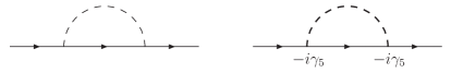
Figure 1: Feynman diagrams for the non-tadpole contributions to $\langle\chi\bar{\chi}\rangle^{(2)}$.

The non-tadpole contributions to the second term of the WTi are (see fig.2)

$$\langle D_{2yz}(A_{z}-i\gamma_{5}B_{z})A_{x}\rangle^{(2)}_{NT}=g^{2}\Big{\{}D_{2yz}\langle A_{z}A_{u}\rangle\Big{[}\mbox{Tr}\Big{(}\langle\chi_{u}\bar{\chi}_{w}\rangle\langle\chi_{w}\bar{\chi}_{u}\rangle\Big{)}+2\langle A_{u}A_{w}\rangle\langle F_{u}F_{w}\rangle$$

$$\phantom{\langle D_{2yz}(A_{z}-i\gamma_{5}}+2\langle B_{u}B_{w}\rangle\langle G_{u}G_{w}\rangle+2\langle F_{u}A_{w}\rangle\langle A_{u}F_{w}\rangle+2\langle B_{u}G_{w}\rangle\langle G_{u}B_{w}\rangle\Big{]}\langle A_{w}A_{x}\rangle$$

$$\phantom{\langle D_{2yz}(A_{z}-i\gamma_{5}}+D_{2yz}\langle A_{z}F_{u}\rangle\Big{[}\langle A_{u}A_{w}\rangle\langle A_{u}A_{w}\rangle+\langle B_{u}B_{w}\rangle\langle B_{u}B_{w}\rangle\Big{]}\langle F_{w}A_{x}\rangle$$

$$\phantom{\langle D_{2yz}(A_{z}-i\gamma_{5}}+2D_{2yz}\langle A_{z}F_{u}\rangle\Big{[}\langle A_{u}A_{w}\rangle\langle A_{u}F_{w}\rangle-\langle B_{u}B_{w}\rangle\langle B_{u}G_{w}\rangle\Big{]}\langle A_{w}A_{x}\rangle$$

$$\phantom{\langle D_{2yz}(A_{z}-i\gamma_{5}}+2D_{2yz}\langle A_{z}A_{u}\rangle\Big{[}\langle A_{u}A_{w}\rangle\langle F_{u}A_{w}\rangle-\langle B_{u}B_{w}\rangle\langle G_{u}B_{w}\rangle\Big{]}\langle F_{w}A_{x}\rangle\Big{\}}\,.$$ (9)

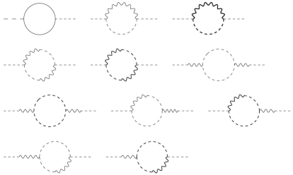
Figure 2: Non-tadpole contributions to $\langle D_{2}(A-i\gamma_{5}B)A\rangle^{(2)}$.

The non-tadpole contributions to the third term of WTi are (see fig.3)

$$\langle(F_{y}-i\gamma_{5}G_{y})A_{x}\rangle^{(2)}_{NT}=g^{2}\Big{\{}2\langle F_{y}A_{u}\rangle\Big{[}\frac{1}{2}\mbox{Tr}\Big{(}\langle\chi_{u}\bar{\chi}_{w}\rangle\langle\chi_{w}\bar{\chi}_{u}\rangle\Big{)}+\langle F_{u}F_{w}\rangle\langle A_{u}A_{w}\rangle$$

$$\phantom{\langle(F_{y}-i\gamma_{5}G_{y})A_{x}\rangle^{(2)}_{NT}}+\langle F_{u}A_{w}\rangle\langle A_{u}F_{w}\rangle+\langle G_{u}G_{w}\rangle\langle B_{u}B_{w}\rangle+\langle B_{u}G_{w}\rangle\langle G_{u}B_{w}\rangle\Big{]}\langle A_{w}A_{x}\rangle$$

$$\phantom{\langle(F_{y}-i\gamma_{5}G_{y})A_{x}\rangle^{(2)}_{NT}}+\langle F_{y}F_{u}\rangle\Big{[}\langle A_{u}A_{w}\rangle\langle A_{u}A_{w}\rangle+\langle B_{u}B_{w}\rangle\langle B_{u}B_{w}\rangle\Big{]}\langle F_{w}A_{x}\rangle$$

$$\phantom{\langle(F_{y}-i\gamma_{5}G_{y})A_{x}\rangle^{(2)}_{NT}}+2\langle F_{y}A_{u}\rangle\Big{[}\langle F_{u}A_{w}\rangle\langle A_{u}A_{w}\rangle-\langle G_{u}B_{w}\rangle\langle B_{u}B_{w}\rangle\Big{]}\langle F_{w}A_{x}\rangle$$

$$\phantom{\langle(F_{y}-i\gamma_{5}G_{y})A_{x}\rangle^{(2)}_{NT}}+2\langle F_{y}F_{u}\rangle\Big{[}\langle A_{u}A_{w}\rangle\langle A_{u}F_{w}\rangle-\langle B_{u}B_{w}\rangle\langle B_{u}G_{w}\rangle\Big{]}\langle A_{w}A_{x}\rangle$$

$$\phantom{\langle(F_{y}-i\gamma_{5}G_{y})A_{x}\rangle^{(2)}_{NT}}-\gamma_{5}\langle G_{y}B_{w}\rangle\mbox{Tr}\Big{(}\gamma_{5}\langle\bar{\chi}_{w}\chi_{u}\rangle\langle\bar{\chi}_{u}\chi_{w}\rangle\Big{)}\langle A_{u}A_{x}\rangle\Big{\}}\,.$$ (10)

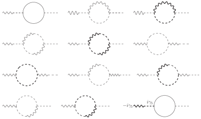
Figure 3: Non-tadpole contributions to $\langle(F-i\gamma_{5}G)A\rangle^{(2)}$.

For the terms of the WTi involving $R$ we find (see fig.4)

$$\langle R_{y}^{(1)}A_{x}\rangle^{(1)}_{NT}=-g\langle\chi\bar{\chi}\rangle_{yz}\times\Big{\{}2\Big{[}\langle A_{z}F_{w}\rangle D_{2zu}\langle A_{u}A_{w}\rangle+\langle A_{z}A_{w}\rangle D_{2zu}\langle A_{u}F_{w}\rangle-D_{2zu}\langle A_{u}F_{w}\rangle\langle A_{u}A_{w}\rangle$$

$$\phantom{\langle R_{y}^{(1)}A_{x}\rangle^{(1)}_{NT}}-\langle B_{z}G_{w}\rangle D_{2zu}\langle B_{u}B_{w}\rangle-\langle B_{z}B_{w}\rangle D_{2zu}\langle B_{u}G_{w}\rangle+D_{2zu}\langle B_{u}B_{w}\rangle\langle B_{u}G_{w}\rangle\Big{]}\langle A_{w}A_{x}\rangle$$

$$\phantom{\langle R_{y}^{(1)}A_{x}\rangle^{(1)}_{NT}}+\Big{[}2\langle A_{z}A_{w}\rangle D_{2zu}\langle A_{u}A_{w}\rangle-D_{2zu}\langle A_{u}A_{w}\rangle\langle A_{u}A_{w}\rangle$$

$$\phantom{\langle R_{y}^{(1)}A_{x}\rangle^{(1)}_{NT}+\Big{[}}+2\langle B_{z}B_{w}\rangle D_{2zu}\langle B_{u}B_{w}\rangle-D_{2zu}\langle B_{u}B_{w}\rangle\langle B_{u}B_{w}\rangle\Big{]}\langle F_{w}A_{x}\rangle\Big{\}}\,.$$ (11)

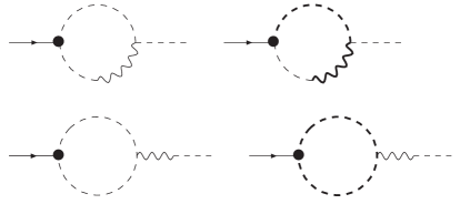
Figure 4: Non-tadpole contributions to $\langle R^{(1)}A\rangle^{(1)}$. The blob denotes the insertion of the operator $D_{2}$.

The last term of WTi is (see fig.5)

$$\langle R_{y}^{(2)}A_{x}\rangle^{(0)}=-\sqrt{2}\langle\chi\bar{\chi}\rangle_{yz}\langle(A_{z}+i\gamma_{5}B_{z})\langle\chi\bar{\chi}\rangle_{zw}\Delta L_{w}A_{x}\rangle^{(0)}$$

$$=-2\Big{\{}\langle\chi_{y}\bar{\chi}_{z}\rangle\langle\chi_{z}\bar{\chi}_{w}\rangle\Big{[}\langle A_{z}A_{w}\rangle D_{2wu}\langle A_{u}A_{x}\rangle+\langle A_{w}A_{x}\rangle D_{2wu}\langle A_{z}A_{u}\rangle-D_{2wu}\langle A_{z}A_{u}\rangle\langle A_{u}A_{x}\rangle\Big{]}$$

$$-\langle\chi_{y}\bar{\chi}_{z}\rangle\gamma_{5}\langle\chi_{z}\bar{\chi}_{w}\rangle\gamma_{5}\Big{[}\langle B_{z}B_{w}\rangle D_{2wu}\langle A_{u}A_{x}\rangle+\langle A_{w}A_{x}\rangle D_{2wu}\langle B_{z}B_{u}\rangle-D_{2wu}\langle B_{z}B_{u}\rangle\langle A_{u}A_{x}\rangle\Big{]}\Big{\}}\,.$$ (12)

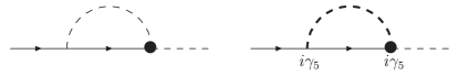
Figure 5: Non-tadpole contributions to $\langle R^{(2)}A\rangle^{(0)}$.

In order to verify Eq. (6) it is convenient to work in the momentum space representation; then we can verify that Eq. (6) is exactly satisfied at fixed lattice spacing [5]. As a last point, let us study the limit $a\to 0$ of Eq. (6) and discuss how this Eq. looks like in the continuum limit, how continuum supersymmetry is restored and the role of the operator $\langle RA\rangle$. Following the notation of Ref. [10] the continuum limit of the fermion two point function reads [5]

$$\langle\chi\bar{\chi}\rangle^{(2)}(p)=\frac{(i/\!\!\!p{}-m)}{(p^{2}+m^{2})}C_{2}i/\!\!\!p{}\frac{(i/\!\!\!p{}-m)}{(p^{2}+m^{2})}$$ (13)

where

$$C_{2}=g^{2}\int\frac{d^{4}k}{(2\pi)^{4}}\frac{\omega^{\prime}_{k}\sin^{2}(k_{\rho})}{[(\omega+b)^{\prime}_{k}+\frac{a^{2}m^{2}}{4}(\omega-b)^{\prime}_{k}]^{3}}+C_{2f}$$ (14)

and $C_{2f}$ is a finite number while $\omega^{\prime}_{k}\equiv a\omega(k/a)=\bigg{[}1-4\sum_{\mu}\sin^{4}(\frac{k_{\mu}}{2})+4\bigg{(}\sum_{\mu}\sin^{2}(\frac{k_{\mu}}{2})\bigg{)}^{2}\bigg{]}^{1/2}$ and $b^{\prime}_{k}\equiv\bigg{[}\sum_{\mu}2\sin^{2}(\frac{k_{\mu}}{2})-1\bigg{]}$. For the scalar two point function we obtain

$$D_{2}\langle AA\rangle^{(2)}(p)=i/\!\!\!p{}\frac{1}{(p^{2}+m^{2})}\frac{1}{(p^{2}+m^{2})}(\frac{1}{2}C_{3}m^{2}-C_{1}p^{2})$$ (15)

where

$$C_{3}=g^{2}\int\frac{d^{4}k}{(2\pi)^{4}}\frac{(\omega^{\prime}_{k})^{2}}{[(\omega^{\prime}+b^{\prime})_{k}+\frac{a^{2}m^{2}}{4}(\omega^{\prime}-b^{\prime})_{k}]^{2}}\,,$$ (16)

$$C_{1}=g^{2}\int\frac{d^{4}k}{(2\pi)^{4}}\frac{\sin^{2}(k_{\rho})\cos(k_{\rho})}{[(\omega^{\prime}+b^{\prime})_{k}+\frac{a^{2}m^{2}}{4}(\omega^{\prime}-b^{\prime})_{k}]^{3}}+C_{1f}$$ (17)

and $C_{1f}$ is a finite constant. A similar analysis applied as before gives

$$\langle FA\rangle^{(2)}(p)=m\frac{1}{(p^{2}+m^{2})}\frac{1}{(p^{2}+m^{2})}(\frac{1}{2}C_{3}+C_{1})p^{2}\,.$$ (18)

The continuum limit of the two point function containing the operator $R$ are

$$\langle R^{(1)}A\rangle^{(1)}(p)=m\frac{(i/\!\!\!p{}-m)}{(p^{2}+m^{2})}\frac{1}{(p^{2}+m^{2})}(C_{2}-\frac{1}{2}C_{3})i/\!\!\!p{}$$ (19)

and

$$\langle R^{(2)}A\rangle^{(0)}(p)=\frac{(i/\!\!\!p{}-m)}{(p^{2}+m^{2})}\frac{1}{(p^{2}+m^{2})}(C_{2}-C_{1})p^{2}\,.$$ (20)

The combinations $C_{2}-C_{1}$ and $C_{2}-\frac{1}{2}C_{3}$ are two (different) finite numbers. Indeed, the $\log(a^{2}m^{2})$ contributions cancels out in these combinations.

Substituting all terms in Eq. (6) with the corresponding signs we have

$$\frac{(i/\!\!\!p{}-m)}{(p^{2}+m^{2})}(i/\!\!\!p{}C_{2})\frac{(i/\!\!\!p{}-m)}{(p^{2}+m^{2})}-\frac{i/\!\!\!p{}}{(p^{2}+m^{2})}(\frac{1}{2}m^{2}C_{3}-p^{2}C_{1})\frac{1}{(p^{2}+m^{2})}$$

$$-\frac{m}{(p^{2}+m^{2})}(C_{1}+\frac{1}{2}C_{3})p^{2}\frac{1}{(p^{2}+m^{2})}+\frac{(i/\!\!\!p{}-m)}{(p^{2}+m^{2})}(i/\!\!\!p{}m)(C_{2}-\frac{1}{2}C_{3})\frac{1}{(p^{2}+m^{2})}$$

$$+\frac{(i/\!\!\!p{}-m)}{(p^{2}+m^{2})}(C_{2}-C_{1})p^{2}\frac{1}{(p^{2}+m^{2})}=0\,.$$ (21)

Notice that the pieces coming from the term $\langle RA\rangle$ above are essential to satisfy the WTi. Thanks to the exactness of WTi it is always possible to write the two point function $\langle RA\rangle$ as a suitable combination of the other three two point functions involved in this WTi. In particular, in the continuum limit one can write

$$\langle RA\rangle=\frac{i/\!\!\!p{}-m}{p^{2}+m^{2}}i/\!\!\!p{}\delta_{1}\frac{i/\!\!\!p{}-m}{p^{2}+m^{2}}+i/\!\!\!p{}\frac{1}{p^{2}+m^{2}}(\delta_{2}p^{2}+\delta_{3}m^{2})\frac{1}{p^{2}+m^{2}}-\frac{m}{p^{2}+m^{2}}(\delta_{2}-\delta_{3})p^{2}\frac{1}{p^{2}+m^{2}}$$ (22)

where $\delta_{1}=\frac{1}{2}C_{3}-C_{2}-\delta_{3}$ and $\delta_{2}=\frac{1}{2}C_{3}-C_{1}-\delta_{3}$, and the constant $\delta_{3}$ is arbitrary. Then in the continuum limit one can rewrite the WTi as the supersymmetric continuum WTi [5]

$$\langle\chi\bar{\chi}\rangle_{R}^{(2)}-i/\!\!\!p{}\langle AA\rangle_{R}^{(2)}-\langle FA\rangle_{R}^{(2)}=0$$ (23)

with $\langle\chi\bar{\chi}\rangle_{R}^{(2)}\equiv\langle\chi\bar{\chi}\rangle^{(2)}+\frac{i/\!\!\!p{}-m}{p^{2}+m^{2}}i/\!\!\!p{}\delta_{1}\frac{i/\!\!\!p{}-m}{p^{2}+m^{2}}$, $\langle AA\rangle_{R}^{(2)}\equiv\langle AA\rangle_{(2)}-\frac{1}{p^{2}+m^{2}}(\delta_{2}p^{2}+\delta_{3}m^{2})\frac{1}{p^{2}+m^{2}}$ and $\langle FA\rangle_{R}^{(2)}\equiv\langle FA\rangle^{(2)}+\frac{m}{p^{2}+m^{2}}(\delta_{2}-\delta_{3})p^{2}\frac{1}{p^{2}+m^{2}}$. It is convenient to express these two point functions in terms of the 1PI vertex functions (just because we started from an off-shell formulation) $\langle\chi\bar{\chi}\rangle^{(2)}=\frac{i/\!\!\!p{}-m}{p^{2}+m^{2}}\,\Sigma^{(2)}_{\chi\bar{\chi}}\,\frac{i/\!\!\!p{}-m}{p^{2}+m^{2}}$, $\langle AA\rangle^{(2)}=-\frac{1}{p^{2}+m^{2}}(\Sigma^{(2)}_{AA}+m^{2}\Sigma^{(2)}_{FF})\frac{1}{p^{2}+m^{2}}$ and $\langle FA\rangle^{(2)}=\frac{1}{p^{2}+m^{2}}(\Sigma^{(2)}_{AA}-p^{2}\Sigma^{(2)}_{FF})\frac{m}{p^{2}+m^{2}}$.

The lattice contribution to these 1PI vertices in the continuum limit reads $\Sigma^{(2)}_{\chi\bar{\chi}}=i/\!\!\!p{}C_{2}$, $\Sigma^{(2)}_{AA}=p^{2}C_{1}$ and $\Sigma^{(2)}_{FF}=-\frac{1}{2}C_{3}$. Moreover, one has $\Sigma^{(2)}_{\chi\bar{\chi}\,R}\equiv\Sigma^{(2)}_{\chi\bar{\chi}}+i/\!\!\!p{}\delta_{1}=i/\!\!\!p{}(\frac{C_{3}}{2}-\delta_{3})\equiv-Z_{\chi}i/\!\!\!p{}$, $\Sigma^{(2)}_{AA\,R}\equiv\Sigma^{(2)}_{AA}+p^{2}\delta_{2}=p^{2}(\frac{C_{3}}{2}-\delta_{3})\equiv-Z_{A}p^{2}$ and $\Sigma^{(2)}_{FF\,R}\equiv\Sigma^{(2)}_{FF}+\delta_{3}=-(\frac{C_{3}}{2}-\delta_{3})\equiv Z_{F}$, with

$$Z_{\chi}=Z_{A}=Z_{F}=-(\frac{C_{3}}{2}-\delta_{3})\,.$$ (24)

In the formulation of Fujikawa (without the $R$), the two-point functions of $A$, $F$ and $\chi$ have the same logarithmic divergent parts [11] but they differ from different finite contributions. An important consequence of the exact lattice supersymmetry we have introduced is that automatically leads to restoration of supersymmetry in the continuum limit with equal renormalization wave function for the scalar and fermion fields.

References

References

[1] G. Curci and G. Veneziano, Nucl. Phys. B292 (1987) 555;
I. Campos et al., Eur. Phys. J. C11 (1999) 507;
I. Montvay, Int. J. Mod. Phys. A17 (2002) 2377.
[2] A. Feo, Nucl. Phys. Proc. Suppl. 119 (2003) 198;
A. Feo, Mod. Phys. Lett. A19 (2004) 2387.
[3] D. B. Kaplan, Nucl. Phys. Proc. Suppl. 29 (2004) 109;
D. B. Kaplan et al., JHEP 0305 (2003) 037; S. Catterall, PoS LAT2005 (2005) 006;
S. Catterall, JHEP 0411 (2004) 006; S. Catterall, JHEP 0506 (2005) 027.
F. Sugino, JHEP 0501 (2005) 016; F. Sugino, JHEP 0403 (2004) 067.
A. D’Adda, I. Kanamori, N. Kawamoto, K. Nagata, hep-lat/0507029;
A. D’Adda, I. Kanamori, N. Kawamoto, K. Nagata, Nucl. Phys. B707 (2005) 100.
[4] M. Bonini and A. Feo, JHEP 0409 (2004) 011.
[5] M. Bonini and A. Feo, Phys. Rev. D69 (2004) 095010.
[6] K. Fujikawa, Nucl. Phys. B636 (2002) 80;
K. Fujikawa and M. Ishibashi, Phys. Lett. B528 (2002) 295.
[7] H. Neuberger, Phys. Lett. B417 (1998) 141;
H. Neuberger, Phys. Lett. B427 (1998) 353.
[8] M. Lüscher, Phys. Lett. B428 (1998) 342;
P. Hernandez, K. Jansen, M. Lüscher, Nucl. Phys. B552 (1999) 363.
[9] P. H. Ginsparg and K. G. Wilson, Phys. Rev. D25 (1982) 2649.
[10] Y. Kikukawa and A. Yamada, Phys. Lett. B448 (1999) 265.
[11] K. Fujikawa and M. Ishibashi, Nucl. Phys. B622 (2002) 115.