Quark masses from quenched overlap fermions

Abstract:

We compute light and strange quark masses for quenched overlap fermions at two values of the gauge coupling. The renormalisation is done non-perturbatively. We test the predictions of quenched chiral perturbation theory for the quark mass dependence of the hadron spectrum and see evidence for the existence of chiral logs.

PoS(LAT2005)077

1 Introduction

Overlap fermions provide the opportunity to investigate QCD at small quark masses. Being computationally extremely expensive, no dynamical results on physically relevant lattices are available yet. In this work, we present spectrum and quark mass results of a quenched study. We calculate light and strange quark masses, and we check several predictions of quenched chiral perturbation theory. Results for nucleon matrix elements are presented in [1].

2 Action, lattices and the scale

Our overlap operator is

$$D=\left(1-\frac{am_{q}}{2\rho}\right)D_{N}+m_{q},\qquad\qquad D_{N}=\frac{\rho}{a}\left(1+{X\left(X^{\dagger}X\right)}^{-1/2}\right),$$ (1)

with the Wilson kernel operator ${X}=D_{W}-\frac{\rho}{a}$. We use a polynomial approximation (see [2]) for ${X\left(X^{\dagger}X\right)}^{-1/2}$, the degree of which is adjusted properly to get an overall residual in the inversion of the overlap better than $10^{-7}$ . The value of $\rho$ is chosen to satisfy the requirements of low condition number and good localisation properties. A way to improve the condition number is the exact treatment of the lowest eigenvalues. Our choice, $\rho=1.4$, is a compromise between small condition number and large localisation mass (i.e. we aim at the upper left hand corner in Fig. 2).

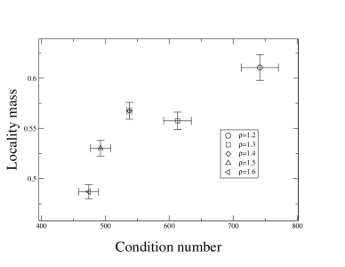
Figure 1: Condition number and localisation mass (1-norm) for $\beta=8.45$, 10 eigenvalues projected out.

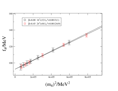
Figure 2: Quenched chiral fits to $f_{\pi}$.

We use the 1-loop tadpole improved Lüscher-Weisz gauge action [3].

$$S[U]=\frac{6}{g^{2}}\left[c_{0}\sum_{\rm plaq}\frac{1}{3}\,\mbox{Re}\,\mbox{Tr}\,(1-U_{\rm plaq})+c_{1}\sum_{\rm rect}\frac{1}{3}\,\mbox{Re}\,\mbox{Tr}\,(1-U_{\rm rect})+c_{2}\sum_{\rm par}\frac{1}{3}\,\mbox{Re}\,\mbox{Tr}\,(1-U_{\rm par})\right].$$ (2)

The lattice gauge coupling $\beta$ is defined as $\beta=6c_{0}/g^{2}$, and the values of $c_{1}$ and $c_{2}$ are fixed by the value of $c_{0}$ and the plaquette expectation value $u_{0}$. The benefits of the Lüscher-Weisz compared to the Wilson gauge action are a better condition number of $X^{\dagger}X$ (as long as no gauge smearing is involved) and absence of dislocations.

We use Jacobi smeared sources ($\kappa=0.21$, $n=50$). To set the scale we compute

$$f_{\pi}(m_{q})=\frac{m_{q}}{m_{\pi}^{3/2}}\frac{A_{sl}}{\sqrt{A_{ss}}},$$ (3)

for each of our quark masses, where $m_{\pi}$ and $A_{sl,ss}$ are the mass and amplitude from cosh fits to the smeared-local and smeared-smeared pseudoscalar correlators. We extrapolate the lattice numbers to the chiral limit by the leading order formula

$$f_{\pi}(m_{q})=f_{\pi}\;\left(1+4L_{5}^{q}\frac{m_{\pi}^{2}}{f_{\pi}^{2}}\right),$$ (4)

The resulting values of $a$ are given in Table 1 (for the values of $L_{5}^{q}$ see the legend of Fig. 2). Note, that the lattice constant is about $10\%$ larger than in [4] where the Sommer scale was used. Such a scale ambiguity is a familiar phenomenon of quenched simulations.

$\beta$	lattice	cfg.	$a/\;\mathrm{fm}$	$a^{-1}/\;\mathrm{MeV}$
8.0	$16^{3}\times 32$	$230$	$0.153(3)$	$1290(30)$
8.45	$16^{3}\times 32$	$250$	$0.105(2)$	$1870(40)$
8.45	$24^{3}\times 48$	$200$	$0.105(1)$	$1870(20)$

Table 1: Lattices used in the simulation. The scale was determined via $f_{\pi}$ (see Fig. 2).

3 Quark masses

The best signal for the pseudoscalar mass is obtained from the correlator of the time component of the axial current. An example of the results is displayed in Fig. 4.

Figure 3: The squared pseudoscalar mass as function of $m_{q}$ together wit the fit Eq. (6).

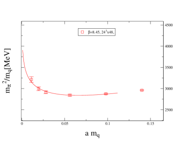
Figure 4: A plot of $m_{\pi}^{2}/m_{q}$ reveals the existence of quenched chiral logs.

The quenched chiral perturbation theory prediction for $m_{\pi}$ reads

$$m_{\pi}^{2}=Am_{q}\left(1-\delta\left(\ln\left(Am_{q}/\Lambda_{\chi}^{2}\right)+1\right)\right)+{\cal O}\left(m_{q}^{2}\right),$$ (5)

where the quenched chiral log appears with a prefactor $\delta$ giving rise to a singularity in $m_{\pi}^{2}/m_{q}$. The fit is shown in Fig. 4. Fixing $\Lambda_{\chi}$ to $1\;\mathrm{GeV}$, we obtain the values of $\delta$ in Table 2.

lattice	$\delta$
$8.00,\,16^{3}\times 32$	$0.16(4)$
$8.45,\,16^{3}\times 32$	$0.3(1)$
$8.45,\,24^{3}\times 48$	$0.15(3)$

Table 2: The chiral log parameter $\delta$.

Although the chiral logs will strongly affect the determination of $m_{\ell}=1/2(m_{u}+m_{d})$, we will ignore this problem in the following.

The fit functions we use to determine the bare light and strange quark masses are

$$m_{\pi}^{2} = Am_{\ell}+Bm_{\ell}\ln m_{\ell}+Cm_{\ell}^{2},$$

$$m_{K}^{2} = A\frac{m_{\ell}+m_{s}}{2}+B\frac{m_{\ell}+m_{s}}{2}\left(\frac{m_{s}\ln m_{s}-m_{\ell}\ln m_{\ell}}{m_{s}-m_{\ell}}-1\right)+C\left({\frac{m_{\ell}+m_{s}}{2}}\right)^{2}.$$ (6)

The renormalisation is done non-pertubatively in the $RI^{\prime}-MOM$ scheme with a variant of the method introduced in [6], using momentum sources[7]. This variant requires only small statistics, and one does not need to perform inversions for each operator under investigation (although one needs to invert the Dirac operator for each momentum separately). We implement the renormalisation condition for the vertex

$$\mbox{Tr}\left(\Gamma_{O}^{{\mathrm{ren}}}\Gamma_{O,{\mathrm{Born}}}^{-1}\right)=12,$$ (7)

on the lattice. Putting in the definition of the renormalised vertex we obtain

$$\frac{1}{Z_{m}}=Z_{S}=\frac{Z_{q}}{\frac{1}{12}\mbox{Tr}\left(\Gamma_{S}\Gamma_{S,{\mathrm{Born}}}^{-1}\right)}.$$ (8)

In the following, we use $\Lambda_{O}$ for the denominator of the r.h.s of Eq. (8) for $O=\{A,V,P,S\}$. The wave function renormalisation $Z_{q}$ is computed from $Z_{q}=Z_{A}\Lambda_{A}$, where we use the axial Ward identity to compute $Z_{A}$, so that it can be extrapolated

$$Z_{A}=\lim_{m_{q}\to 0}\lim_{t\to\infty}\frac{2m_{q}\left<P\left(t\right)P\left(0\right)\right>}{\left<\partial_{4}A_{4}\left(t\right)P\left(0\right)\right>}.$$ (9)

The chiral extrapolation is illustrated in Fig. 6.

Figure 5: $Z_{A}$ from the axial Ward identity.

Figure 6: $Z_{S}^{\mathrm{RGI}}$ for both values of $\beta$

We now proceed with the computation of $\Lambda_{A}$and $\Lambda_{S}$. We exploit the identity is $\Lambda_{S}=\Lambda_{P}$, a consequence of chiral symmetry. On the lattice both are modified by zero mode effects $\propto 1/(am_{q})^{2}$, which are finite volume artefacts. Additionally, spontaneous chiral symmetry breaking produces a $1/(am_{q})$ contribution to $\Lambda_{P}^{\mathrm{latt}}$. Thus, we extract $\Lambda_{S}$ as the common constant from fits

$$\Lambda_{P}^{\mathrm{latt}} = \frac{p_{1}}{a^{2}m_{q}^{2}}+\frac{p_{2}}{am_{q}}+\Lambda_{S}+p_{4}a^{2}m_{q}^{2},$$

$$\Lambda_{S}^{\mathrm{latt}} = \frac{s_{1}}{a^{2}m_{q}^{2}}+\Lambda_{S}+s_{3}a^{2}m_{q}^{2}.$$ (10)

for each value of $\mu^{2}$. $\Lambda_{A}$ is computed in a similar fashion from linear fits to $\Lambda_{A}^{\mathrm{latt}}$ and $\Lambda_{V}^{\mathrm{latt}}$ with a common constant. In the next step we need to identify the region where non-perturbative effects are small. To this end we remove the renormalisation group running from the $RI^{\prime}-MOM$ renormalisation constant $Z_{S}=Z_{A}\Lambda_{A}/\Lambda_{S}$ using the 4-loop results from [8]. The result is shown in Fig. 6, where the linear regions are clearly identified. We extract the intercept and quote the results in the ${\overline{MS}}$ scheme at $\mu=2\;\mathrm{GeV}$ in Table 4.

$\beta$	$Z_{S}^{RGI}$	slope	$Z_{S}^{\overline{MS}}(2\;\mathrm{GeV}$)
$8.00$	$1.18(2)$	$-0.007(2)$	$0.85(2)$
$8.45$	$1.02(1)$	$-0.004(1)$	$0.73(1)$

Table 3: $Z_{S}$

$\beta$	$m_{\ell}^{{\overline{MS}}}$	$m_{s}^{{\overline{MS}}}$
$8.00$	$4.2(1)$	$127(1)$
$8.45,16^{3}\,32$	$3.5(2)$	$118(3)$
$8.45,24^{3}\,48$	$4.1(1)$	$119(1)$

Table 4: Light and strange quark masses

Note, that the lattice artefacts (represented by the slope) scale with $a^{2}$, as expected for (the automatically ${\cal{O}}(a)$ improved) overlap fermions. The resulting quark masses are given in Table 4. The light quark mass scales very well, but we see a volume dependence. For the strange quark mass we see some dependence on $a$, but not on the volume.

4 Vector meson and nucleon masses

In this section we extract vector meson and nucleon masses from our data and compare their chiral behaviour to predictions of quenched chiral perturbation theory. The vector meson mass (Fig. 8) confirms the prediction of a negative value of $C_{1/2}$ in a fit according to $m_{\rho}(m_{\pi})=m_{\rho}+C_{1/2}m_{\pi}+C_{1}m_{\pi}^{2}+C_{3/2}m_{\pi}^{3}$.

Figure 7: Quenched chiral fits to the vector meson.

Figure 8: The same for the nucleon. The dashed line is a fit to low mode averaged data.

The prediction for the nucleon has the same structure, but it is harder to confirm the negative sign of $C_{1/2}$ for $m_{N}$, since the errors make the results compatible with zero unless one uses the low mode averaging technique. In this case we find a value of $C_{1/2}=-0.32(18)$ at $\beta=8.45$, $24^{3}\,48$, which is in good agreement with the chiral perturbation theory prediction $C_{1/2}=3/2\pi(D-3F)^{2}\delta=-0.25(5)$ (Fig. 8).

5 Summary

In a quenched overlap simulation we have computed the light and strange quark masses $m_{\ell}^{\overline{MS}}(2\;\mathrm{GeV})=4.1(1)\;\mathrm{MeV}$ and $m_{s}^{\overline{MS}}(2\;\mathrm{GeV})=119(1)\;\mathrm{MeV}$. We demonstrated the existence of quenched chiral logs and the expected chiral behaviour of $f_{\pi}$, $m_{\rho}$, and $m_{N}$.

6 Acknowledgements

The numerical calculations were performed at the IBM pSeries 690 computers at HLRN and NIC Jülich, and on the PC farm at DESY Zeuthen.We thank these institutions for their support. Part of this work is supported by the DFG under contract FOR465.

References

- [1] QCDSF Collaboration, T. Streuer et. al., Nucleon structure from quenched overlap fermions, PoS(LAT2005)363 (these proceedings).
- [2] L. Giusti, C. Hoelbling, M. Lüscher and H. Wittig, Numerical techniques for lattice QCD in the - regime, Comput. Phys. Commun. 153 (2003) 31–51 [hep-lat/0212012].
- [3] M. Lüscher and P. Weisz, On-shell improved lattice gauge theories, Commun. Math. Phys. 97 (1985) 59.
- [4] C. Gattringer, R. Hoffmann and S. Schaefer, Setting the scale for the Lüscher-Weisz action, Phys. Rev. D65 (2002) 094503 [hep-lat/0112024].
- [5] QCDSF Collaboration, R. Horsley, H. Perlt, P. E. L. Rakow, G. Schierholz and A. Schiller, One-loop renormalisation of quark bilinears for overlap fermions with improved gauge actions, Nucl. Phys. B693 (2004) 3–35 [hep-lat/0404007]. Erratum-ibid. B713 (2005) 601.
- [6] G. Martinelli, C. Pittori, C. T. Sachrajda, M. Testa and A. Vladikas, A General method for nonperturbative renormalization of lattice operators, Nucl. Phys. B445 (1995) 81–108 [hep-lat/9411010].
- [7] M. Göckeler et. al., Nonperturbative renormalisation of composite operators in lattice QCD, Nucl. Phys. B544 (1999) 699–733 [hep-lat/9807044].
- [8] J. A. Gracey, Three loop anomalous dimension of non-singlet quark currents in the scheme, Nucl. Phys. B662 (2003) 247–278 [hep-ph/0304113].
- [9] R. L. Jaffe and A. Manohar, The g(1) problem: fact and fantasy on the spin of the proton, Nucl. Phys. B337 (1990) 509–546.