DESY 05-228, Edinburgh 2005/20, LU-ITP 2005/023, LTH 683
Perturbative Renormalisation for Low Moments of Generalised Parton Distributions with Clover Fermions

Abstract

We present the non-forward quark matrix elements of operators with one and two covariant derivatives needed for the renormalisation of the first and second moments of generalised parton distributions in one-loop lattice perturbation theory using clover fermions. For some representations of the hypercubic group commonly used in simulations we define the sets of possible mixing operators and compute the one-loop mixing matrices of renormalisation factors. Tadpole improvement is applied to the results and some numerical examples are presented.

1 INTRODUCTION

Generalised parton distributions (GPDs) have become a focus of both experimental and theoretical studies in hadron physics (for an extensive up-to-date review see [1]). They allow a parametrisation of a large class of hadronic correlators, including e.g. form factors and the ordinary parton distribution functions. Thus GPDs provide a solid formal basis to connect information from various inclusive, semi-inclusive and exclusive reactions in an efficient, unambiguous manner. Furthermore they give access to physical quantities which cannot be directly determined in experiments, like e.g. the orbital angular momentum of quarks and gluons in a nucleon (for a chosen specific scheme) and the spatial distribution of the energy or spin density of a fast moving hadron in the transverse plane. Since the structure of GPDs is rather complicated a direct experimental access is limited. Therefore, complementary information channels have to be opened up. One major source is lattice QCD [2, 3, 4, 5, 6].

Recently [7] we have calculated the non-forward matrix elements in one-loop lattice perturbation theory for the Wilson fermion action needed for the renormalisation of the second moments of GPDs. From these results the renormalisation factors for various representations of the hypercubic group have been derived.

Here we present some new results for operators with two covariant derivatives using the Sheikholeslami-Wohlert (clover) action [8], which leads to $O(a)$ improved quark-quark-gluon and quark-quark-gluon-gluon vertices in the Feynman rules. Since in current numerical simulations the operators for the second moment of GPDs are not improved, we ignore such a possible additional improvement. Note that the $O(a)$ improvement for operators with one covariant derivative is known [9].

We consider the Wilson gauge action and clover fermions with the fermionic action $S_{\rm SW,F}$ [8] (for dimensionful massless fermion fields $\psi(x)$)

$$S_{\rm SW,F} = 4ra^{3}\sum_{x}\bar{\psi}(x)\psi(x)$$

$$- \frac{a^{3}}{2}\sum_{x,\mu}\left[\bar{\psi}(x)(r-\gamma_{\mu})U_{x,\mu}\psi(x+a\hat{\mu})\right.$$

$$+ \left.\bar{\psi}(x+a\hat{\mu})(r+\gamma_{\mu})U^{\dagger}_{x,\mu}\psi(x)\right]$$

$$- \frac{a^{4}\,g\,c_{sw}}{4}\sum_{x,\mu,\nu}\,\bar{\psi}(x)\sigma_{\mu\nu}F^{\rm clover}_{\mu\nu}\psi(x)\,.$$

Here $a$ denotes the lattice spacing and the sums run over all lattice sites $x$ and directions $\mu,\nu$ (all other indices are suppressed). $F^{\rm clover}_{\mu\nu}$ is the standard “clover-leaf” form of the lattice field strength and $\sigma_{\mu\nu}=i/2[\gamma_{\mu},\gamma_{\nu}]$.

In a perturbative calculation the operators to be investigated are sandwiched between off-shell quark states with 4-momenta $p$ and $p^{\prime}$. Our calculations are performed in Feynman gauge, the final numbers are presented for the Wilson parameter $r=1$, leaving the value of $c_{sw}$ free.

One-link quark operators with clover fermions have been discussed in [9] for forward matrix elements. The renormalisation constants found there for a given representation of the hypercubic group H(4) and charge conjugation parity $C$ can be used in the non-forward case as well. Additionally, in the case of GPDs “transversity” operators have to be taken into account. We will collect here all results for completeness.

It is well known that operators with two or more covariant derivatives may mix under H(4): the one- and higher-loop structures differ in general from that of the Born term and multiplicative renormalisation may get lost. In addition, for non-forward matrix elements also operators with ordinary (external) derivatives can contribute making the mixing problem more complicated. To find the possible candidates for mixing one has to define those operators which belong to the same irreducible representation under H(4) and have the same charge conjugation parity.

We define renormalised operators $\mathcal{O}_{i}^{\cal S}$ by

$${\cal O}_{i}^{\cal S}(\mu)=\sum_{k=1}^{N}Z_{ik}^{S}(a,\mu)\,{\cal O}_{k}(a)$$ (2)

where $\mathcal{S}$ denotes the renormalisation scheme and $N$ is the number of operators which mix in one-loop. $Z_{ik}^{\mathcal{S}}(a,\mu)$ are the renormalisation constants connecting the lattice operator $\mathcal{O}_{k}(a)$ with the renormalised operator $\mathcal{O}_{i}^{\mathcal{S}}(\mu)$ at scale $\mu$. We present the renormalisation constants in the $\overline{MS}$ scheme following [7].

2 OERATORS AND MIXING

We consider operators with up to two covariant symmetric lattice derivatives $\stackrel{{\scriptstyle\leftrightarrow}}{{D}}=\stackrel{{\scriptstyle\rightarrow}}{{D}}-\stackrel{{\scriptstyle\leftarrow}}{{D}}$ and external ordinary derivatives $\partial$ needed for the chosen representations of interest for the first and second moment of GPDs. The standard realisation of the covariant derivatives acting to the right and to the left is used:

$$\stackrel{{\scriptstyle\rightarrow}}{{D}}_{\mu}\psi(x)=\frac{1}{2a}\times$$ (3)

$$\Big{[}U_{x,\mu}\,\psi(x+a\hat{\mu})-U^{\dagger}_{x-a\hat{\mu},\mu}\,\psi(x-a\hat{\mu})\Big{]}\,,$$

$$\bar{\psi}(x)\stackrel{{\scriptstyle\leftarrow}}{{D}}_{\mu}=\frac{1}{2a}\times$$ (4)

$$\Big{[}\bar{\psi}(x+a\hat{\mu})\,U^{\dagger}_{x,\mu}-\bar{\psi}(x-a\hat{\mu})\,U_{x-a\hat{\mu},\mu}\Big{]}\,.$$

The external ordinary derivative is taken as

$$\partial_{\mu}\left(\bar{\psi}\cdots\psi\right)\!(x)=\frac{1}{a}\times$$ (5)

$$\Big{[}\left(\bar{\psi}\cdots\psi\right)(x+a\hat{\mu})-\left(\bar{\psi}\cdots\psi\right)\!(x)\Big{]}\,.$$

The number of derivatives appearing in the operators is indicated by superscripts $D$ and $\partial$, respectively. Quark operators with one derivative are given by

$$\mathcal{O}^{D}_{\mu\nu} = -\frac{i}{2}\bar{\psi}\gamma_{\mu}\stackrel{{\scriptstyle\leftrightarrow}}{{D}}_{\nu}\psi\,,$$ (6)

$$\mathcal{O}^{5,D}_{\mu\nu} = -\frac{i}{2}\bar{\psi}\gamma_{\mu}\gamma_{5}\stackrel{{\scriptstyle\leftrightarrow}}{{D}}_{\nu}\psi\,,$$ (7)

$$\mathcal{O}^{T,D}_{\mu\nu\omega} = -\frac{i}{2}\bar{\psi}[\gamma_{\mu},\gamma_{\nu}]\stackrel{{\scriptstyle\leftrightarrow}}{{D}}_{\omega}\psi\,,$$ (8)

$$\mathcal{O}^{T,\partial}_{\mu\nu\omega} = -\frac{i}{2}\partial_{\omega}\left(\bar{\psi}[\gamma_{\mu},\gamma_{\nu}]\psi\right)\,.$$ (9)

The operator (8) is a transversity operator antisymmetric in its first two indices which is of interest for GPDs, operators (8) and (9) contribute as lower dimensional operators to mixing in certain representations of the second moment of GPDs.

As operators with two derivatives we consider here

$$\mathcal{O}_{\mu\nu\omega}^{DD} = -\frac{1}{4}\bar{\psi}\gamma_{\mu}\stackrel{{\scriptstyle\leftrightarrow}}{{D}}_{\nu}\stackrel{{\scriptstyle\leftrightarrow}}{{D}}_{\omega}\psi\,,$$

$$\mathcal{O}_{\mu\nu\omega}^{\partial D} = -\frac{1}{4}\partial_{\nu}\left(\bar{\psi}\gamma_{\mu}\stackrel{{\scriptstyle\leftrightarrow}}{{D}}_{\omega}\psi\right)\,,$$ (10)

$$\mathcal{O}_{\mu\nu\omega}^{\partial\partial} = -\frac{1}{4}\partial_{\nu}\partial_{\omega}\left(\bar{\psi}\gamma_{\mu}\psi\right)\,.$$

In addition, spin-dependent and “transversity” operators have to be considered when discussing all possible representations. They are roughly obtained by replacing $\gamma_{\mu}$ by $\gamma_{\mu}\gamma_{5}$ and $\sigma_{\mu\tau}$, respectively.

To define the various representations with given $C$ we use the following short-hand notations

$$\mathcal{O}_{\cdots\{\nu_{1}\nu_{2}\}} = \frac{1}{2}\left(\mathcal{O}_{\cdots\nu_{1}\nu_{2}}+\mathcal{O}_{\cdots\nu_{2}\nu_{1}}\right)\,,$$

$$\mathcal{O}_{\{\nu_{1}\nu_{2}\nu_{3}\}} = \frac{1}{6}\left(\mathcal{O}_{\nu_{1}\nu_{2}\nu_{3}}+\mathcal{O}_{\nu_{1}\nu_{3}\nu_{2}}+\mathcal{O}_{\nu_{2}\nu_{1}\nu_{3}}\right.$$

$$+ \left.\mathcal{O}_{\nu_{2}\nu_{3}\nu_{1}}+\mathcal{O}_{\nu_{3}\nu_{1}\nu_{2}}+\mathcal{O}_{\nu_{3}\nu_{2}\nu_{1}}\right)\,,$$

$$\mathcal{O}_{\|\nu_{1}\nu_{2}\nu_{3}\|} = \mathcal{O}_{\nu_{1}\nu_{2}\nu_{3}}-\mathcal{O}_{\nu_{1}\nu_{3}\nu_{2}}$$

$$+ \mathcal{O}_{\nu_{3}\nu_{1}\nu_{2}}-\mathcal{O}_{\nu_{3}\nu_{2}\nu_{1}}-2\,\mathcal{O}_{\nu_{2}\nu_{3}\nu_{1}}$$

$$+ 2\,\mathcal{O}_{\nu_{2}\nu_{1}\nu_{3}}\,,$$

$$\mathcal{O}_{\langle\langle\nu_{1}\nu_{2}\nu_{3}\rangle\rangle} = \mathcal{O}_{\nu_{1}\nu_{2}\nu_{3}}+\mathcal{O}_{\nu_{1}\nu_{3}\nu_{2}}$$

$$- \mathcal{O}_{\nu_{3}\nu_{1}\nu_{2}}-\mathcal{O}_{\nu_{3}\nu_{2}\nu_{1}}\,.$$

Let us denote an irreducible representation of the hypercubic group $H(4)$ by $\tau_{k}^{(l)}$ with dimension $l$ ($k$ labels inequivalent representations of the same dimension) and a given charge conjugation parity $C$ by $\pm 1$.

For the first moments we choose the following representations presented in Table 1 (for the notation and a detailed discussion of the transformation under H(4) see [10]). They are renormalised multiplicatively.

Table 1: Operators and their transformation under the hypercubic group.

Operator	$\tau_{k}^{(l)}$	$C$
$\mathcal{O}^{D}_{\{14\}}$	$\tau_{3}^{(6)}$	$+1$
$\mathcal{O}^{D}_{44}-\frac{1}{3}\left(\mathcal{O}^{D}_{11}+\mathcal{O}^{D}_{22}+\mathcal{O}^{D}_{33}\right)$	$\tau_{1}^{(3)}$	$+1$
$\mathcal{O}^{5,D}_{\{14\}}$	$\tau_{4}^{(6)}$	$-1$
$\mathcal{O}^{5,D}_{44}-\frac{1}{3}\left(\mathcal{O}^{5,D}_{11}+\mathcal{O}^{5,D}_{22}+\mathcal{O}^{5,D}_{33}\right)$	$\tau_{4}^{(3)}$	$-1$
$\mathcal{O}^{T,D}_{\langle\langle 124\rangle\rangle}$	$\tau_{2}^{(8)}$	$+1$
$\mathcal{O}^{T,D}_{\langle\langle 122\rangle\rangle}-\mathcal{O}^{T,D}_{\langle\langle 133\rangle\rangle}$	$\tau_{1}^{(8)}$	$+1$
$\mathcal{O}^{T,D}_{\|122\|}-\mathcal{O}^{T,D}_{\|133\|}$	$\tau_{1}^{(8)}$	$-1$

For the second moments we consider in this contribution the following mixing cases ( the details and additional operators will be presented elsewhere [11]):
Representation $\tau_{2}^{(4)}$, $C=-1$ with operators

$$\mathcal{O}_{\{124\}}^{DD}\,,\,\mathcal{O}_{\{124\}}^{\partial\partial}\,.$$ (11)

Representation $\tau_{1}^{(8)}$, $C=-1$ with

$$\mathcal{O}_{1}=\mathcal{O}^{DD}_{\{114\}}-\frac{1}{2}\left(\mathcal{O}^{DD}_{\{224\}}+\mathcal{O}^{DD}_{\{334\}}\right)\,,$$

$$\mathcal{O}_{2}=\mathcal{O}^{\partial\partial}_{\{114\}}-\frac{1}{2}\left(\mathcal{O}^{\partial\partial}_{\{224\}}+\mathcal{O}^{\partial\partial}_{\{334\}}\right)\,,$$

$$\mathcal{O}_{3}=\mathcal{O}^{DD}_{\langle\langle 114\rangle\rangle}-\frac{1}{2}\left(\mathcal{O}^{DD}_{\langle\langle 224\rangle\rangle}+\mathcal{O}^{DD}_{\langle\langle 334\rangle\rangle}\right)\,,$$

$$\mathcal{O}_{4}=\mathcal{O}^{\partial\partial}_{\langle\langle 114\rangle\rangle}-\frac{1}{2}\left(\mathcal{O}^{\partial\partial}_{\langle\langle 224\rangle\rangle}+\mathcal{O}^{\partial\partial}_{\langle\langle 334\rangle\rangle}\right)\,,$$

$$\mathcal{O}_{5}=\mathcal{O}^{5,\partial D}_{||213||}\,,\quad\mathcal{O}_{6}=\mathcal{O}^{5,\partial D}_{\langle\langle 213\rangle\rangle}\,,$$ (12)

$$\mathcal{O}_{7}=\mathcal{O}^{5,DD}_{||213||}\,,$$

$$\mathcal{O}_{8}=\mathcal{O}^{T,\partial}_{411}-\frac{1}{2}\left(\mathcal{O}^{T,\partial}_{422}+\mathcal{O}^{T,\partial}_{433}\right)\,.$$

3 ONE-LOOP CALCULATION

We calculate the non-forward matrix elements of the operators in one-loop lattice perturbation theory in the infinite volume limit following Kawai et al. [12]. Details of the computational procedure are given in [7].

In lattice momentum space operators with non-zero momentum transfer $q$ are realised by applying the lattice momentum transfer $q$ at the lattice position $x$ or at the “position centre” $x+\frac{a}{2}\hat{\mu}$, e.g. for an operator with one covariant derivative we have the two possibilities

$$\left(\bar{\psi}\stackrel{{\scriptstyle\leftrightarrow}}{{D}}_{\!\mu}\,\psi\right)\!(q)=\frac{1}{2a}\sum_{x}\left\{{\rm e}^{iq\cdot x}+{\rm e}^{iq\cdot(x+a\hat{\mu})}\atop 2{\rm e}^{iq\cdot(x+a\hat{\mu}/2)}\right\}\times$$

$$\left[\bar{\psi}(x)U_{x,\mu}\psi(x+a\hat{\mu})-\bar{\psi}(x+a\hat{\mu})U^{\dagger}_{x,\mu}\psi(x)\right]\,.$$ (13)

Eq. (3) basically defines the Feynman rules for the operators in lattice perturbation theory. As an example we get for the operator $\mathcal{O}^{DD}_{\mu\nu\omega}$ to order $O(g^{0})$ ($g$ is the bare gauge coupling):

$${\cal O}^{DD}_{\mu\nu\omega}(p^{\prime},p)=\bar{\psi}(p^{\prime})\gamma_{\mu}\psi(p)\,\times$$

$$\frac{1}{a}\sin\frac{a(p+p^{\prime})_{\nu}}{2}\,\frac{1}{a}\sin\frac{a(p+p^{\prime})_{\omega}}{2}\times$$ (14)

$$\left\{{\cos\frac{a(p-p^{\prime})_{\nu}}{2}\,\cos\frac{a(p-p^{\prime})_{\omega}}{2}\atop 1}\right\}\,.$$

In the following sections we denote the upper/lower realisations by supercripts $I/II$.

The contributing one-loop diagrams for the self energy and the amputated Green (vertex) functions are shown in Figures 1 and  2 (filled black circles indicate the place of the operator insertions):

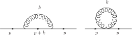
Figure 1: Quark self energy diagrams.

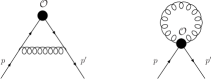
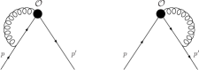
Figure 2: Amputated Green function diagrams.

3.1 First Moment

Since mixing is absent, we omit the matrix notation for the renormalisation constants and use the general form ($C_{F}=4/3$, $g_{R}$ is the renormalised coupling)

$$Z(a\mu)=1-\frac{g_{R}^{2}\,C_{F}}{16\pi^{2}}\left[\gamma\,\ln(a^{2}\mu^{2})+B(c_{sw})\right]$$ (15)

with the anomalous dimensions $\gamma=8/3$ for the first four operators and $\gamma=2$ for the last three operators in Table 1. For the operators of that Table we get the finite contributions shown in Table 2.

Table 2: Finite contributions $B(c_{sw})$ for the first moments.

Representation	$B(c_{sw})$
$\tau_{3}^{(6)}$	$1.280-3.873\,c_{sw}-0.678\,c_{sw}^{2}$
$\tau_{1}^{(3)}$	$2.562-3.970\,c_{sw}-1.040\,c_{sw}^{2}$
$\tau_{4}^{(6)}$	$0.345-1.359\,c_{sw}-1.893\,c_{sw}^{2}$
$\tau_{4}^{(3)}$	$0.167-1.249\,c_{sw}-1.998\,c_{sw}^{2}$
$\tau_{2}^{(8)}$	$13.169+2.675\,c_{sw}-1.494\,c_{sw}^{2}$
$\tau_{1}^{(8)}$ ($C=\pm 1$)	$12.804+2.624\,c_{sw}-1.430\,c_{sw}^{2}$

3.2 Second Moment

We present the matrix of renormalisation constants in the generic form

$$Z_{ij}^{(m)}(a\mu) =$$ (16)

$$\delta_{ij}-\frac{g_{R}^{2}\,C_{F}}{16\pi^{2}}\left[\gamma_{ij}\,\ln(a^{2}\mu^{2})+B_{ij}^{(m)}(c_{sw})\right]$$

with

$$B_{ij}^{(m)}(c_{sw})=B_{ij}^{(0,m)}+B_{ij}^{(1,m)}\,c_{sw}+B_{ij}^{(2,m)}\,c_{sw}^{2}\,.$$

The superscript $(m)$ with $m=I,II$ distinguishes the realisations I and II of the covariant derivatives (3).

Representation $\tau_{2}^{(4)}$, $C=-1$

For this representation the operators (11) mix. The corresponding $2\times 2$-mixing matrices are

$$\gamma_{jk}=\left(\begin{array}[]{rr}\frac{25}{6}&-\frac{5}{6}\\ 0&0\end{array}\right)\,,$$ (17)

$$B_{jk}^{(I,II)}(c_{sw})=\left(\begin{array}[]{rr}-11.563&0.024\\ 0&20.618\end{array}\right)$$ (20)

$$\hskip 54.06023pt+\left(\begin{array}[]{rr}2.898&-0.255\\ 0&4.746\end{array}\right)\,c_{sw}$$ (23)

$$\hskip 54.06023pt-\left(\begin{array}[]{rr}0.984&\hskip 8.53581pt0.016\\ 0&0.543\end{array}\right)\,c_{sw}^{2}\,.$$ (26)

In the matrix $B_{jk}^{(I,II)}$ the mixing between the operators $\mathcal{O}_{\{124\}}^{DD}$ and $\mathcal{O}^{\partial\partial}_{\{124\}}$ is very small. Thus it may be justified to neglect the mixing in practical applications.

Representation $\tau_{1}^{(8)}$, $C=-1$

We consider the mixing (2) of the operators having the same dimension first. These are the operators $\mathcal{O}_{1}\dots\mathcal{O}_{7}$ in (2). To one-loop accuracy the operator $\mathcal{O}_{7}$ does not contribute and we have to consider the following mixing set:

$$\{\mathcal{O}_{1},\mathcal{O}_{2},\mathcal{O}_{3},\mathcal{O}_{4},\mathcal{O}_{5},\mathcal{O}_{6}\}\,.$$

The anomalous dimension matrix is

$$\gamma_{jk}=\left(\begin{array}[]{rrrrrr}\frac{25}{6}&-\frac{5}{6}&0&0&0&0\\ 0&0&0&0&0&0\\ 0&0&\frac{7}{6}&-\frac{5}{6}&1&-\frac{3}{2}\\ 0&0&0&0&0&0\\ 0&0&0&0&2&-2\\ 0&0&0&0&-\frac{2}{3}&\frac{2}{3}\end{array}\right)$$ (27)

and the finite parts of the mixing matrix are given in Table 3. (in cases of doublets the upper number belongs to type I, the lower to type II of realisation of lattice covariant derivative).

Table 3: Finite parts of the mixing matrix for operators of representation $\tau_{1}^{(8)}$, $C=-1$.

$$B_{jk}^{(0,I,II)} = \left(\begin{array}[]{rrrrrr}-12.127&\left(\begin{array}[]{r}1.491\\ -2.737\end{array}\right)&0.368&\left(\begin{array}[]{r}0.015\\ 0.994\end{array}\right)&0.016&0.150\\[8.61108pt] 0&20.618&0&0&0&0\\[8.61108pt] 3.306&\left(\begin{array}[]{r}-8.015\\ 18.184\end{array}\right)&-14.852&\left(\begin{array}[]{r}4.431\\ -4.302\end{array}\right)&-0.928&0.738\\[8.61108pt] 0&0&0&20.618&0&0\\ 0&3.264&0&0&0.350&0.015\\ 0&3.264&0&0&0.005&0.360\end{array}\right)$$

$$\hskip 34.1433ptB_{jk}^{(1,I,II)} = \left(\begin{array}[]{rrrrrr}2.922&\left(\begin{array}[]{r}-0.213\\ -0.686\end{array}\right)&-0.033&\left(\begin{array}[]{r}0.015\\ 0.173\end{array}\right)&-0.019&0.057\\[8.61108pt] 0&4.746&0&0&0&0\\[8.61108pt] 0.333&\left(\begin{array}[]{r}-0.766\\ -0.055\end{array}\right)&2.152&\left(\begin{array}[]{r}1.206\\ 0.970\end{array}\right)&-1.758&2.298\\[8.61108pt] 0&0&0&4.746&0&0\\ 0&-1.441&0&0&1.648&0.866\\ 0&-1.441&0&0&0.289&2.225\end{array}\right)$$

$$B_{jk}^{(2,I,II)} = \left(\begin{array}[]{rrrrrr}-0.982&\left(\begin{array}[]{r}-0.078\\ -0.101\end{array}\right)&-0.029&\left(\begin{array}[]{r}0.035\\ 0.042\end{array}\right)&-0.001&0.007\\[8.61108pt] 0&-0.543&0&0&0&0\\[8.61108pt] 0.371&\left(\begin{array}[]{r}-0.551\\ 0.215\end{array}\right)&-1.707&\left(\begin{array}[]{r}0.371\\ 0.116\end{array}\right)&-0.443&0.103\\[8.61108pt] 0&0&0&-0.543&0&0\\ 0&1.416&0&0&-1.703&0.568\\ 0&1.416&0&0&0.189&-1.325\end{array}\right)$$

Using lattice perturbation theory to one-loop, $1/a$ terms may appear when calculating the matrix elements of the operators with two covariant derivatives. Such terms are potentially dangerous because of the power-law divergence in the continuum limit. Considering the representation $\tau_{2}^{(4)}$, a potential mixing is absent. On the contrary, we get mixing for operator ${\cal O}_{1}$ of $\tau_{1}^{(8)}$ with the lower dimensional operator $\mathcal{O}_{8}$ given in (2). The perturbative mixing result is

$${\cal O}_{1}\big{|}_{1/a-{\rm part}}=\frac{g_{R}^{2}C_{F}}{16\pi^{2}}\,\frac{1}{a}\,{\cal O}_{8}^{{\rm tree}}\times$$ (37)

$$(-0.518+0.0832\,c_{sw}-0.00983\,c_{sw}^{2})\,,$$

but a nonperturbative subtraction from the matrix element of ${\cal O}_{1}$ is required to obtain reliable numbers.

4 TADPOLE IMPROVEMENT AND SOME NUMERICAL EXAMPLES

Since many results of (naive) lattice perturbation theory are in bad agreement with their numerical counterparts, it has has been proposed [13] to rearrange the (naive) lattice perturbative series. This rearrangement is performed using the variable $u_{0}$ (the mean field value of the link), e.g. defined from the measured value of the plaquette at a given coupling

$$u_{0}=\langle\frac{1}{3}{\rm Tr}U_{\Box}\rangle^{\frac{1}{4}}\,.$$ (38)

In case of mixing the tadpole improvement procedure proceeds as follows. By scaling the link variables $U_{\mu}$ with $u_{0}$

$$U_{\mu}(x)=u_{0}\,\left(\frac{U_{\mu}(x)}{u_{0}}\right)=u_{0}\,\overline{U}_{\mu}(x)$$

the amputated Green function for operator $\mathcal{O}$ with $n$ covariant derivatives $\Lambda^{(n)}_{\mathcal{O}}$ takes the form

$$\Lambda^{(n)}_{\mathcal{O}}=u_{0}^{n}\Lambda^{(n)}_{\mathcal{O}}(\overline{U}_{\mu}(x))\,.$$ (39)

$\Lambda^{(n)}_{\mathcal{O}}(\overline{U}_{\mu}(x))$ is expected to have a better converging perturbative expansion. Up to order $g^{2}$ we obtain for the Wilson gauge action, labelling the operators by $i$ and the corresponding number of covariant derivatives by $n_{i}$,

$$\Lambda^{(n_{i})}_{i}(\overline{U}_{\mu}(x)) = \left(\frac{1}{u_{0}^{n_{i}}}\right)_{\rm pert}\,\Lambda^{(n_{i})}_{i,{\rm pert}}(U_{\mu}(x))$$ (40)

$$= \left(1+\frac{g^{2}C_{F}}{16\,\pi^{2}}\,n_{i}\,\pi^{2}+O(g^{4})\right)$$

$$\times\left(\Lambda^{(n_{i},{\rm tree})}_{i}+\frac{g^{2}C_{F}}{16\,\pi^{2}}\sum_{k=1}^{n}w_{ik}\Lambda^{(n_{k},{\rm tree})}_{k}\right.$$

$$\left.+O(g^{4})\right)\,,$$

where the $w_{ik}$ denote the mixing weights. From (40) it becomes clear that in one-loop only the diagonal terms in the mixing matrix get a shift proportional to $n_{i}\,\pi^{2}$. An external ordinary derivative ($\partial$) does not provide a factor of $u_{0}$. Taking into account the mean field value for the wave function renormalisation constant for massless Wilson fermions $Z_{\psi,{\rm Wilson}}^{MF}=u_{0}$ we get the tadpole improved matrix of renormalisation constants in the form

$$Z_{ij}^{TI} = u_{0}^{1-n_{i}}\times$$ (41)

$$\left(1-\frac{g^{2}C_{F}}{16\,\pi^{2}}(n_{i}-1)\,\pi^{2}\,\delta_{ij}+O(g^{4})\right)\,Z_{ij}\,.$$

Additionally, one has to replace the parameters $g$ and $c_{sw}$ by their boosted counterparts

$$g_{TI}^{2}\equiv g^{2}\,u_{0}^{-4}\,,\quad c_{sw}^{TI}\equiv c_{sw}\,u_{0}^{3}\,.$$ (42)

Putting (16), (41) and (42) together we obtain for the tadpole improved renormalisation mixing matrix in one-loop order

$$Z_{ij}^{TI,(m)} = u_{0}^{1-n_{i}}\,\bigg{(}\delta_{ij}-\frac{g_{TI}^{2}\,C_{F}}{16\pi^{2}}\times$$ (43)

$$\Big{(}\gamma_{ij}\,\ln(a^{2}\mu^{2})+B_{ij}^{TI,(m)}(c_{sw}^{TI})\Big{)}\bigg{)}$$

with

$$B_{ij}^{TI,(m)}(c_{sw}^{TI})=B_{ij}^{(m)}(c_{sw}^{TI})+(n_{i}-1)\pi^{2}\,\delta_{ij}\,.$$ (44)

Let us demonstrate the effect of tadpole improvement by some numerical examples. We choose $a=1/\mu$, $\beta=6$, $u_{0}=0.8778$ and $c_{sw}=1+O(g^{2})$ [9]. For the first moments the only effect consists in replacing $c_{sw}$ by $c_{sw}^{TI}$ and $g_{R}$ by $g_{TI}$ in (15) and in Table 2. For the representation $\tau_{3}^{(6)}$ we get

$$Z=1.028\quad\rightarrow\quad Z^{TI}=1.023\,.$$ (45)

For the second moments we consider the simple mixing $\mathcal{O}_{\{124\}}^{DD}\leftrightarrow\mathcal{O}_{\{124\}}^{\partial\partial}$ (11) first. Without tadpole improvement we obtain the mixing matrix

$$Z_{ij}=\left(\begin{array}[]{rr}1.081&0.002\\ 0&0.790\end{array}\right)\,.$$ (46)

The tadpole improved result is

$$Z_{ij}^{TI}=\left(\begin{array}[]{rr}1.142&0.002\\ 0&0.707\end{array}\right)\,.$$ (47)

It might be instructive to compare the one-loop corrections for the renormalisation constants: $B^{(m)}_{ij}(c_{sw})$ for the unimproved case (16) and $B_{ij}^{TI,(m)}(c_{sw}^{TI})$ for the tadpole improved case (43). We get

$$B_{ij}=\left(\begin{array}[]{rr}-9.649&-0.247\\ 0&24.821\end{array}\right)$$ (48)

and

$$B_{ij}^{TI}=\left(\begin{array}[]{rr}-0.209&-0.177\\ 0&12.035\end{array}\right)\,.$$ (49)

We observe that in agreement with the improvement aims the diagonal one-loop contributions are reduced.

For the representation $\tau_{1}^{(8)}$, $C=-1$ with the mixing of operators $\mathcal{O}_{1}\dots\mathcal{O}_{6}$ we obtain for the unimproved/improved mixing matrices (choosing $m=I$) the numbers given in Table 4.

Table 4: Unimproved and improved mixing matrices for the representation $\tau_{1}^{(8)}$, $C=-1$ at $a=1/\mu$, $\beta=6$, $u_{0}=0.8778$ and $c_{sw}=1+O(g^{2})$.

$$Z_{ij}^{(I)} = \left(\begin{array}[]{rrrrrr}1.086&-0.010&-0.003&-0.001&0.0&-0.002\\ 0&0.790&0&0&0&0\\ -0.034&0.079&1.122&-0.051&0.026&-0.027\\ 0&0&0&0.790&0&0\\ 0&-0.027&0&0&0.998&-0.012\\ 0&-0.027&0&0&-0.004&0.989\end{array}\right)$$

$$\hskip 56.9055ptZ_{ij}^{TI,(I)} = \left(\begin{array}[]{rrrrrr}1.151&-0.021&-0.005&-0.001&0.0&-0.003\\ 0&0.707&0&0&0&0\\ -0.060&0.142&1.209&-0.088&0.037&-0.038\\ 0&0&0&0.707&0&0\\ 0&-0.042&0&0&0.990&-0.012\\ 0&-0.042&0&0&-0.004&0.982\end{array}\right)$$

5 SUMMARY

Within the framework of lattice QCD with clover improved Wilson fermions and Wilson’s plaquette action for the gauge fields we have calculated the one-loop quark matrix elements of operators needed for the first two moments of GPDs and meson distribution amplitudes. From these we have determined the matrices of renormalisation and mixing coefficients in the $\overline{MS}$-scheme.

For the first moments of GPDs we can use the results from the first moments of structure functions. The results for the second moments extend the numbers obtained with Wilson fermions [7]. The general conclusions concerning the mixing properties remain unchanged. All sets which consist of one operator with two covariant derivatives $D$ and one operator with two external derivatives $\partial$ show very small mixing. The set discussed here with seven potential candidates (2) shows a more significant mixing.

Moreover, taking $\mathcal{O}_{1}$ from (2) as the operator to be measured in a numerical simulation a mixing with a lower dimensional operator $\mathcal{O}_{8}$ appears. This requires a nonperturbative subtraction for Wilson or clover fermions.

Using overlap fermions, such a mixing with a dangerous lower dimensional operator must be absent, since the mixing operators are of different chirality.

References

• [1] M. Diehl, Phys. Rept.  388 (2003) 41 [arXiv:hep-ph/0307382].
• [2] P. Hägler, J. Negele, D. B. Renner, W. Schroers, T. Lippert and K. Schilling [LHPC collaboration], Phys. Rev. D 68 (2003) 034505 [arXiv:hep-lat/0304018].
• [3] M. Göckeler, R. Horsley, D. Pleiter, P. E. L. Rakow, A. Schäfer, G. Schierholz and W. Schroers [QCDSF Collaboration], Phys. Rev. Lett.  92 (2004) 042002 [arXiv:hep-ph/0304249].
• [4] M. Göckeler, Ph. Hägler, R. Horsley, D. Pleiter, P.E.L. Rakow, A. Schäfer, G. Schierholz and J.M. Zanotti Nucl. Phys. Proc. Suppl.  140 (2005) 399 [arXiv:hep-lat/0409162].
• [5] M. Göckeler, Ph. Hägler, R. Horsley, D. Pleiter, P.E.L. Rakow, A. Schäfer, G. Schierholz and J.M. Zanotti Nucl. Phys. A 755 (2005) 537 [arXiv:hep-lat/0501029].
• [6] M. Göckeler, Ph. Hägler, R. Horsley, D. Pleiter, P.E.L. Rakow, A. Schäfer, G. Schierholz and J.M. Zanotti Phys.  Lett.   B 627 (2005) 113 [arXiv:hep-lat/0507001].
• [7] M. Göckeler, R. Horsley, H. Perlt, P. E. L. Rakow, A. Schäfer, G. Schierholz and A. Schiller, Nucl. Phys. B 717 (2005) 304 [arXiv:hep-lat/0410009].
• [8] B. Sheikholeslami and R. Wohlert, Nucl. Phys. B 259 (1985) 572.
• [9] S. Capitani, M. Göckeler, R. Horsley, H. Perlt, P. E. L. Rakow, G. Schierholz and A. Schiller, Nucl. Phys. B 593 (2001) 183 [arXiv:hep-lat/0007004].
• [10] M. Göckeler, R. Horsley, E.-M. Ilgenfritz, H. Perlt, P. Rakow, G. Schierholz and A. Schiller, Phys. Rev. D 54 (1996) 5705 [arXiv:hep-lat/9602029].
• [11] M. Göckeler, R. Horsley, H. Perlt, P. E. L. Rakow, A. Schäfer, G. Schierholz and A. Schiller, in preparation.
• [12] H. Kawai, R. Nakayama and K. Seo, Nucl. Phys. B 189 (1981) 40.
• [13] G. P. Lepage and P. B. Mackenzie, Phys. Rev. D 48 (1993) 2250.