A lattice calculation of the pion form factor with Ginsparg-Wilson-type fermions

Abstract

Results for Monte Carlo calculations of the electromagnetic vector and scalar form factors of the pion in a quenched simulation are presented. We work with two different lattice volumes up to a spatial size of 2.4 fm at a lattice spacing of 0.148 fm. The pion form factors in the space-like region are determined for pion masses down to 340 MeV.

I Introduction

The ab-initio determination of hadronic properties is an important task of lattice QCD calculations. Following the impressive progress in the determination of the hadron mass spectrum, one went on to more advanced calculations, such as the determination of matrix elements. An important example is the electromagnetic pion form factor MaSa88 ; DrWoWi89 ; Ne04 ; HeKoLa04 ; BoEdFl05 ; AbLe05 ; Br05 .

With the successful implementation of chiral symmetry, based on the Ginsparg-Wilson (GW) relation GiWi82 , also results at smaller quark masses are feasible. In addition to an exact implementation NaNe93a95 ; Ne9898a , further Dirac operators have been suggested that fulfill the GW condition in an approximate way, among them the domain-wall fermions Ka92 ; FuSh95 , the perfect fermions HaNi94 and the chirally improved (CI) fermions Ga01 ; GaHiLa00 .

Dynamical calculations at small quark masses are certainly the ultimate goal. Currently such calculations are still prohibitively expensive but one can try to improve in two ways: either one works with dynamical fermions in a conventional formulation or one tries to approach smaller quark masses with GW type operators in the quenched approximation. In our present contribution we focus on the latter.

We present here a first-principles calculation for off-forward lattice matrix elements of operators that measure the vector and scalar form factors of the pion. We work with the CI fermions, which constitute an approximate solution of the Ginsparg-Wilson relation and thus have improved chiral properties GaGoHa03a . In our calculation we consider comparatively low pion masses down to 340 MeV, which is likely in the domain where chiral perturbation theory (ChPT) can be applied. Another convenient feature of chirally improved fermions is that the renormalization of the local current $Z_{V}$ is quite close to 1 GaGoHu04 .

Preliminary results of our calculations have been presented in Ref. CaGaLa05a . The quenched results for the vector form factor at the available transferred momenta lie close to the experimental curves. From our data for the form factors we can derive the charge radius of the pion as well as its scalar radius. The former comes out smaller than experiment, due to the too large value of the $\rho$-meson mass. The scalar radius appears to be sensitive to quenching and possibly to the contributions of the disconnected diagrams, which we do not include in our calculations.

The pion form factor in the quenched approximation has been studied for Wilson type fermions MaSa88 ; DrWoWi89 ; HeKoLa04 ; BoEdFl05 ; Br05 , for GW type fermions Ne04 and for twisted mass fermions AbLe05 . There are few results for dynamical fermions: for Wilson-type fermions in Refs. HaAoFu05 ; Br05 , and a study with domain-wall valence quarks and dynamical (MILC) Asqtad fermions BoEdFl05 (and further references therein).

II Pion form factors

The vector form factor $F_{\pi}$ is defined by

$$\langle\pi^{+}(\mathbf{p}_{f})|\,V_{\mu}\,|\pi^{+}(\mathbf{p}_{i})\rangle_{\textrm{\scriptsize cont}}=(p_{f}+p_{i})_{\mu}\,F_{\pi}(Q^{2})\;,$$ (1)

where $Q^{2}=(p_{f}-p_{i})^{2}\equiv-t$ is the space-like invariant momentum transfer squared, and

$$V_{\mu}=\frac{2}{3}\;\overline{u}\,\gamma_{\mu}\,u-\frac{1}{3}\;\overline{d}\,\gamma_{\mu}\,d$$ (2)

is the vector current.

The pion vector form factor is an analytic function of $t$. Its space-like values are determined from the values on the boundary of its analyticity domain, i.e., the cut along the positive real $t$-axis. Although it starts at $t=4\,m_{e}^{2}$, significant contributions only come from the hadronic region, starting with the two-pion threshold at $4\,m_{\pi}^{2}$. Along the first part of the cut, until inelastic channels become important, due to unitarity the phase shift is essentially the p wave phase shift of the elastic two-pion channel. That region is dominated by the $\rho$-meson resonance. This feature has been exploited by various dispersion relation representations GoSa68 ; HeLa81 ; TrYn02 ; Le02 .

Although there are further inelastic contributions from the four-pion channel, these remain tiny until the $\pi\omega$ channel opens. There is also a small contribution from the isoscalar $\omega$, coupling through higher-order electromagnetic interactions. All these contributions show small effects on the near space-like region and can be safely neglected within the accuracy attained in our work.

The dominant contribution of the vector meson resonances has inspired the vector meson dominance (VMD) model, where the form factor in the space-like domain is approximated by a sum of poles in the time-like region,

$$F_{\pi}^{VMD}=\sum_{V}\frac{f_{V\pi\pi}}{f_{V\gamma}}\frac{m_{V}^{2}}{m_{V}^{2}-t}\;.$$ (3)

In first approximation the coefficients are related to the coupling $f_{V\pi\pi}$ of the vector meson to the two-pion state and its coupling to the photon, $f_{V\gamma}$.

In QCD the large $Q^{2}$ behavior in leading order FaJa79 is given by

$$F_{\pi}(Q^{2})\sim\frac{8\,\pi\,\alpha_{s}(Q^{2})\,f_{\pi}^{2}}{Q^{2}}\;,$$ (4)

with $\alpha_{s}$ the running coupling constant (logarithmic in the argument) and $f_{\pi}$ the pion decay constant. In the $Q^{2}$-region accessible to us the logarithm is not identifiable and the VMD behavior provides a good approximation.

Due to electric charge conservation one has $F_{\pi}(0)=1$. The mean charge radius squared is defined through

$$F_{\pi}(Q^{2}) = 1-\frac{1}{6}\,\langle r^{2}\rangle_{\textrm{\scriptsize v}}\,Q^{2}+{\cal O}\big{(}Q^{4}\big{)}$$ (5)

$$\rightarrow \langle r^{2}\rangle_{\textrm{\scriptsize v}}\equiv 6\,dF_{\pi}(t)/dt|_{t=0}\;.$$

The current PDG average for its value is $0.45(1)\;\textrm{fm}^{2}$ PDG04 .

In the simplest VMD model with just the leading $\rho$-resonance one has (due to normalization) $f_{\rho\pi\pi}=f_{\rho\gamma}$ and

$$F_{\pi}(Q^{2}) = {m_{\rho}^{2}}/({m_{\rho}^{2}-t})$$ (6)

$$\rightarrow \langle r^{2}\rangle_{\textrm{\scriptsize v,VMD}}=\frac{6}{m_{\rho}^{2}}\approx 0.39\;\textrm{fm}^{2}\;.$$

The scalar form factor $\Gamma_{\pi}$ is given by the matrix element of the scalar operator, i.e.,

$$\langle\pi^{+}(\mathbf{p}_{f})|\,m_{u}\,\overline{u}\,u+m_{d}\,\overline{d}\,d\,|\pi^{+}(\mathbf{p}_{i})\rangle=\Gamma_{\pi}(Q^{2})\;.$$ (7)

Within chiral perturbation theory the scalar form factor at $Q^{2}=0$ is the so-called sigma term which behaves like $\Gamma_{\pi}(0)\sim M_{\pi}^{2}$ near zero momentum transfer. The scalar radius squared $\langle r^{2}\rangle_{s}$ can be obtained from

$$\frac{\Gamma_{\pi}(Q^{2})}{\Gamma_{\pi}(0)}=1-\frac{1}{6}\,\langle r^{2}\rangle_{s}\,Q^{2}+{\cal O}\big{(}Q^{4}\big{)}\;.$$ (8)

For a detailed discussion of chiral perturbation theory in this context see AnCaCo04 .

Figure 1: Schematic diagram for the matrix element (9).

III Strategy

In order to compute the form factors, we need to evaluate off-forward matrix elements (at several transferred momenta), i.e., the expectation values of

$${\mathrm{Tr}}\left[\sum_{\mathbf{y};\,y_{0}=\tau}\!\!\mathrm{e}^{i\,\mathbf{q}\cdot\mathbf{y}}S(0,y)\;O\!\!\sum_{\mathbf{x};\,x_{0}=t}\!\!\mathrm{e}^{-i\,\mathbf{p}\cdot\mathbf{x}}S(y,x)\gamma_{5}S(x,0)\gamma_{5}\right]\;,$$ (9)

where $S(y,x)$ is the quark propagator from $x$ to $y$ and $O$ denotes the operator inserted at $y$. We use the notation $\mathbf{p}\equiv\mathbf{p}_{f}$, $\mathbf{r}\equiv\mathbf{p}_{i}$ and denote the momentum transfer as $\mathbf{q}=\mathbf{p}-\mathbf{r}$ (cf. Fig. 1).

The necessary matrix elements have been evaluated by using the sequential source method. The matrix element is then written as

$$\mathrm{Tr}\,\left[\sum_{\mathbf{y};y_{0}=\tau}\,e^{i\,\mathbf{q}\cdot\mathbf{y}}\,S(0,y)\;O\;\Sigma(y,0)\,\gamma_{5}\right]\;.$$ (10)

The sequential propagator is defined as

$$\Sigma(y,0)=\sum_{\mathbf{x};x_{0}=t}\,e^{-i\,\mathbf{p}\cdot\mathbf{x}}\,S(y,x)\,\gamma_{5}\,S(x,0)\;,$$ (11)

and can be easily computed by an additional inversion of the Dirac operator $D$ for each choice of the final momentum $\mathbf{p}$,

$$\sum_{y}D(z,y)\,\Sigma(y,0)=e^{-i\,\mathbf{p}\cdot\mathbf{z}}\,\gamma_{5}\,S(z,0)\Big{|}_{z_{0}=t}\;.$$ (12)

Changing the properties of the sink requires the computation of new sequential propagators, and so simulating several final momenta, different field interpolators, or a different smearing for the sink rapidly becomes rather expensive. For this reason we have limited ourselves to only one value of the final momentum. An alternative version of the sequential source method, which builds the sequential propagator from the two propagators that sandwich the operator, would allow more values of the final momentum for free, but on the other hand it would require a new inversion of the Dirac operator for every new type of operator and for each different value of the momentum transfer. This is much less convenient in our situation because we consider both the vector and scalar currents and want to obtain the corresponding form factors for several values of the momentum transfer.

We extract the physical matrix elements by computing ratios of 3-point and 2-point correlators:

$$R(t,\tau;\mathbf{p},\mathbf{q})=\frac{\langle P(t;\mathbf{p})\,O(\tau;\mathbf{q})\,\overline{P}(0;\mathbf{r})\rangle}{\langle P(t;\mathbf{p})\,\overline{P}(0;\mathbf{p})\rangle}\,\sqrt{\,\frac{\langle P(t;\mathbf{p})\,\overline{P}(0;\mathbf{p})\rangle\,\langle P(\tau;\mathbf{p})\,\overline{P}(0;\mathbf{p})\rangle\,\langle P(t-\tau;\mathbf{r})\,\overline{P}(0;\mathbf{r})\rangle}{\langle P(t;\mathbf{r})\,\overline{P}(0;\mathbf{r})\rangle\,\langle P(\tau;\mathbf{r})\,\overline{P}(0;\mathbf{r})\rangle\,\langle P(t-\tau;\mathbf{p})\,\overline{P}(0;\mathbf{p})\rangle}}\;,$$ (13)

where $P=\overline{u}\,\gamma_{5}\,d$ is our pseudoscalar interpolator. We keep the sink fixed at time $t$ and vary the timeslice $\tau$ where the operator $O$ sits (scanning a range of timeslices).

The ratio (13) eliminates the exponential factors in the time variable which are present if one considers $\langle P(t;\mathbf{p})\,O(\tau;\mathbf{q})\,\overline{P}(0;\mathbf{r})\rangle$ alone. As a consequence, $R(t,\tau;\mathbf{p},\mathbf{q})$ exhibits two plateaus in $\tau$: $0\ll\tau\ll t$ and $t\ll\tau\ll T$. In the case in which the sink is put at $t=T/2$ the ratio is antisymmetric in $\tau-T/2$.

In the Monte Carlo simulations the momentum projections of the sink onto non-zero $\mathbf{p}$ and the operator onto non-zero momentum transfer $\mathbf{q}$ lead to significant statistical fluctuations due to the worse signal-to noise ratio. In particular, for many configurations the 2-point correlators become negative on timeslices near the symmetry point $t=T/2$. A reasonable way out of this inconvenient situation is to choose the sink to sit at a timeslice smaller than $T/2$, because in this region the 2-point correlators have much larger values, and moreover their relative errors are smaller. We have thus put the sink at timeslice $t=7$, while the source remained at timeslice $t=0$. The matrix elements are finally determined (as in the case $t=T/2$) by combining the two plateau values on either side of the sink, $R_{\textrm{\scriptsize lhs}}\pm R\textrm{\scriptsize rhs}$, where the relative sign depends on the parity properties of the operators. This sign is negative for the vector and positive for the scalar form factor.

The term under the square root in Eq. (13) becomes trivial for $\mathbf{q}=(0,0,0)$. In that case the ratio becomes

$$\frac{\langle P(t;\mathbf{p})\,O(\tau;\mathbf{q}=\mathbf{0})\,\overline{P}(0;\mathbf{r}=\mathbf{p})\rangle}{\langle P(t;\mathbf{p})\,\overline{P}(0;\mathbf{p})\rangle}$$ (14)

and is sufficient to eliminate the exponentials.

Table 1: Values of the non-zero momentum transfers.

size	$\sqrt{2}\,p_{0}$	$2\,p_{0}$	$\sqrt{6}\,p_{0}$	$2\sqrt{2}\,p_{0}$
$16^{3}\times 32$	0.739 GeV	1.045 GeV	1.280 GeV	1.478 GeV
$12^{3}\times 24$	0.986 GeV	1.394 GeV	1.707 GeV	1.971 GeV

We choose momenta $|\mathbf{p}_{f}|=|\mathbf{p}_{i}|$, which implies $E_{f}=E_{i}$ so that the transferred 4-momentum is then given by $Q^{2}=|\mathbf{q}|^{2}$. In this way HeKoLa04 one achieves for the electromagnetic form factor a cancellation of the kinematical factors in (1) and

$$\langle\pi(\mathbf{p}_{f})|V_{\mu}|\pi(\mathbf{p}_{i})\rangle_{\textrm{\scriptsize latt}}=\frac{1}{2\,\sqrt{E_{f}E_{i}}}\langle\pi(\mathbf{p}_{f})|V_{\mu}|\pi(\mathbf{p}_{i})\rangle_{\textrm{\scriptsize cont}}\;.$$ (15)

Indeed, with this choice of momenta, and using the $\mu=4$ component of the vector current, the overall factor becomes

$$\frac{E_{f}+E_{i}}{2\sqrt{E_{f}E_{i}}}=1\;.$$ (16)

This cancellation is unfortunately no longer possible in the calculation of the scalar form factor, where a remaining multiplication by the quantity $2\,\sqrt{E_{f}\,E_{i}}$ is still needed.

In our calculations the pion source is located at the origin and the sink has a non-zero 3-momentum which is fixed to $\mathbf{p}_{f}=(1,1,0)\,p_{0}$, where $p_{0}=2\,\pi/(a\,L)$ denotes the smallest non-vanishing spatial momentum. The momenta of the current are then chosen such that implicitly

$$|\mathbf{p}_{f}|=|\mathbf{p}_{i}|=\sqrt{2}\,p_{0}$$ (17)

is verified. We use twelve different 3-momenta for the current, $(0,0,0)$, $(0,1,\pm 1)$, $(1,0,\pm 1)$, $(2,0,0)$, $(0,2,0)$, $(2,1,\pm 1)$, $(1,2,\pm 1)$, $(2,2,0)$; these are all the possible choices that obey the condition (17). This setup then gives rise to four non-zero (and equidistant) values for the square of the momentum transfer, $Q^{2}=2\,n\,p_{0}^{2}$ for $n=0,\,1,\,2,\,3,\,4$ (see Table 1). Momentum conservation finally defines the twelve corresponding values for the 3-momentum of the source, which all have the same module.

We could also consider larger values of the module of the initial momentum, since this would generate further values of $Q^{2}$ while still using the same sequential propagators through the sink. In this case, however, the statistical errors become much larger, and moreover we could not use Eq. (16) anymore. A change of the momentum at the sink would require the expensive computation of a new set of sequential propagators.

IV Simulation parameters

We use the chirally improved Dirac operator Ga01 ; GaHiLa00 ; GaGoHa03a , which constitutes an approximate Ginsparg-Wilson operator. The gauge action is the Lüscher-Weisz tadpole improved action at $\beta=7.9$ LuWe85 , corresponding to a lattice spacing of 0.148 fm (determined from the Sommer parameter in GaHoSc02 ). Here we do not study the scaling behavior. However, although we cannot estimate the discretization effects, we expect that our results have only small $O(a)$ contributions, because chirally improved fermions are Ginsparg-Wilson-like fermions. This has been observed in the study of the hadron spectrum GaGoHa03a and other hadron properties GaHuLa05 .

The pion interpolators are constructed from Jacobi-smeared quark sources and sinks (with $\kappa=0.21$ and $N=18$), which improves the signal for the ground state.

We performed simulations on two volumes: $12^{3}\times 24$ (200 configurations for each mass) and $16^{3}\times 32$ (100 configurations for each mass). This corresponds to spatial lattice sizes of $a\,L\sim 1.8\;$fm and $a\,L\sim 2.4\;$fm respectively.

We work at several values of the bare quark mass and the corresponding meson masses are given in Table 2 (taken from GaGoHa03a ). The jackknife method is used for estimating the statistical errors of our results.

Table 2: Pion and rho masses at the various quark masses simulated (taken from GaGoHa03a ).

	$16^{3}\times 32$	$16^{3}\times 32$	$16^{3}\times 32$	$12^{3}\times 24$	$12^{3}\times 24$
$m$	0.02 $a^{-1}$	0.04 $a^{-1}$	0.06 $a^{-1}$	0.04 $a^{-1}$	0.06 $a^{-1}$
$m_{\pi}$	342 MeV	471 MeV	571 MeV	474 MeV	575 MeV
$m_{\rho}$	845 MeV	895 MeV	941 MeV	952 MeV	976 MeV

V Results

In order to illustrate the quality of the results, we show in Figs. 2 and 7 the time dependence of the ratio (13). Fitting the central points of the plateaus to a constant then leads to the values for the form factors.

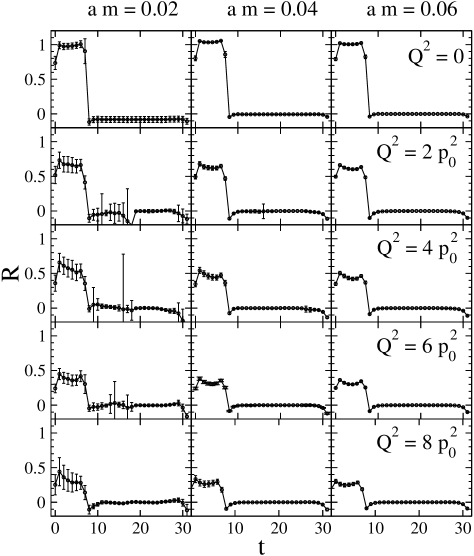
Figure 2: The ratio (13) leading to the vector form factor for all quark masses and transfer momenta considered (lattice size $16^{3}\times 32$).

Table 3: Values of the pion vector form factor (lattice size $16^{3}\times 32$, $a=0.148$ fm) obtained for different quark mass values.

$Q^{2}$[GeV]	$a\,m$=0.02	$a\,m$=0.04	$a\,m$=0.06
0	1.01(1)	0.996(3)	0.963(13)
0.546	0.64(15)	0.596(42)	0.580(23)
1.093	0.54(14)	0.434(42)	0.409(24)
1.639	0.36(12)	0.296(34)	0.289(20)
2.186	0.29(14)	0.252(43)	0.239(25)

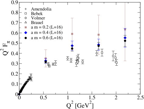
Figure 3: Our results for the pion vector form factor $Q^{2}\,F_{\pi}$ compared with results from experiments (lattice size $16^{3}\times 32$).

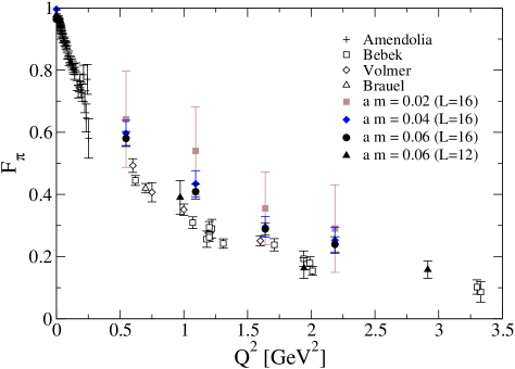
Figure 4: Our results for the pion vector form factor $F_{\pi}$ compared with results from experiments (lattice sizes $16^{3}\times 32$ and $12^{3}\times 24$).

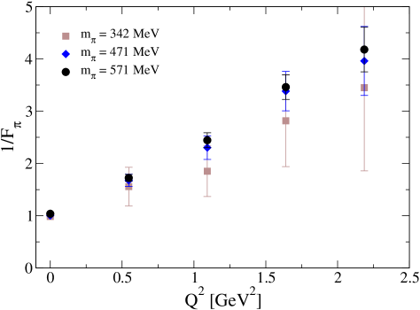
Figure 5: The inverse vector form factor for the three available masses on the $16^{3}\times 32$ lattice.

Some combinations of initial and final momenta induce more statistical noise than others. To increase our statistics we average over all combinations that have the same momentum transfer. In particular, for $Q^{2}=2\,p_{0}^{2}$ and $Q^{2}=6\,p_{0}^{2}$ we have four times as many data, and for $Q^{2}=4\,p_{0}^{2}$ the averaging doubles our statistics.

When comparing the results to physical, renormalized quantities we have to multiply with renormalization factors relating the raw results to the $\overline{\textrm{MS}}$-scheme. For the chirally improved Dirac operator these have been determined in GaGoHu04 and all results we show, except for the plots of the ratios, are already converted to the $\overline{\textrm{MS}}$-scheme. We always use values as determined in the chiral limit.

V.1 Vector form factor

Although the vector current is pointlike and not conserved, the value $Z_{V}=0.9586(2)$ turns out to be close to unity. This number converts the lattice bare results at $a=$ 0.148 fm to the corresponding renormalized continuum quantities in the $\overline{\rm MS}$ scheme at the scale of 2 GeV. The fact that the renormalization constant $Z_{V}$ is so close to 1 means that we have better control over this kind of systematic effects.

The resulting $F_{\pi}(0)$ is not constrained to unit value, but comes very close. This fact is obvious from the results summarized in Table 3. These values have been computed by combining the plateau mean values as discussed before; these have been obtained by averaging the values at $t=3$ and 4 of the l.h.s. plateau and the values at $t=20-23$ of the r.h.s plateau. The errors have been determined with the jackknife method. The larger error bars in some of the plots are an indication of the rather poor signal-to-noise ratio for some timeslices close to the lattice center. These timeslices are however outside the regions that we use for the fits. As already mentioned in Sect. III, we profit from the cancellation of kinematical factors by following the approach suggested in Ref. HeKoLa04 .

Fig. 3 compares our results for the vector form factor with results from experiments Vo01 ; Be78 ; Am86 ; Br79 . In Fig. 4 we show these results together with those for the small lattice size $12^{3}\times 24$. For this smaller lattice size the statistics was sufficient only for the data at $a\,m=0.06$. The resulting form factor values are at other momentum transfer values than those of the larger volume, but in reasonable agreement.

In Fig. 5 we plot the inverse of the vector form factor. The electromagnetic pion form factor in the time-like region is dominated by the $\rho$-meson. In the near space-like region it may therefore be well approximated by a monopole form (6) such that the leading behavior of $1/F_{\pi}$ is linear. This is indeed observed in Fig. 5.

As the VMD model is just an approximation, one expects corrections due to other resonances and more-particle channels in the time-like region. In the fit these may be taken into account by further pole terms. Our data shown in Fig. 5 do not really require such a multi-parameter fit and we therefore discuss only the results of a linear fit.

The derivative of the form factor at $Q^{2}=0$ gives the charge radius, as shown in Fig. 6. The derivative has been obtained from the linear fit to the inverse form factor. Whereas the large mass results are compatible with a constant in $a\,m$, the number for the lowest mass is smaller but has a very large statistical error. These values are quite compatible with numbers from HeKoLa04 at comparable quark masses.

Obviously in our results there is an unknown systematic error due to the quenched approximation. We refrain from applying QChPT extrapolations because the data are not accurate enough to reliably determine the unknown expansion parameters for the non-linear terms. Computing the average gives $\langle r^{2}\rangle_{\textrm{\scriptsize v}}=0.291(18)\;\textrm{fm}^{2}$.

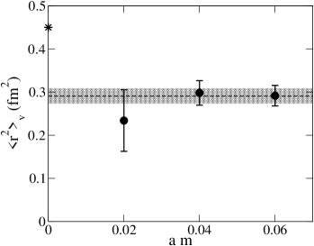
Figure 6: The mean square radius for the vector form factor as obtained for the three available masses on the $16^{3}\times 32$ lattice. The asterisk denotes the average experimental value PDG04 , the error band shows the result of a constant fit to the three points.

The value of $\langle r^{2}\rangle_{\textrm{\scriptsize v}}$ in the VMD model is inversely proportional to the mass squared of the $\rho$-meson. We obtain $m_{\textrm{\scriptsize VMD}}^{2}=0.80(5)\;\textrm{GeV}^{2}$. This agrees with the range of values obtained for $m_{\rho}^{2}$ in the analysis of Ref. GaGoHa03a in the direct $\rho$-channel (e.g., $m_{\rho}^{2}=0.80\;\textrm{GeV}^{2}$ at $a\,m=0.04$). These large values for the $\rho$-meson mass might at least in part explain (via the VMD model) our low (as compared to experiment) result for $\langle r^{2}\rangle_{\textrm{\scriptsize v}}$.

Like most other calculations we could afford only to work for a single value of the lattice spacing and therefore we have no control on scaling violations. However, due to the (approximate) GW nature of the CI operator we expect $\mathcal{O}(a)$ corrections to be very small GaGoHa03a .

Due to the chosen method we have fewer momentum transfer values than BoEdFl05 , who also work at larger lattices and at slightly smaller quark masses. Our results, obtained with different action and Dirac operator, are in generally good agreement with the findings of other lattice calculations in the discussed range of values for mass and momentum transfer BoEdFl05 ; HeKoLa04 , even for those with dynamical background BoEdFl05 . Higher quark masses overestimate the values of the form factor, as it is expected due to the corresponding higher vector meson mass. This then leads to an underestimation of the charge radius.

V.2 Scalar form factor

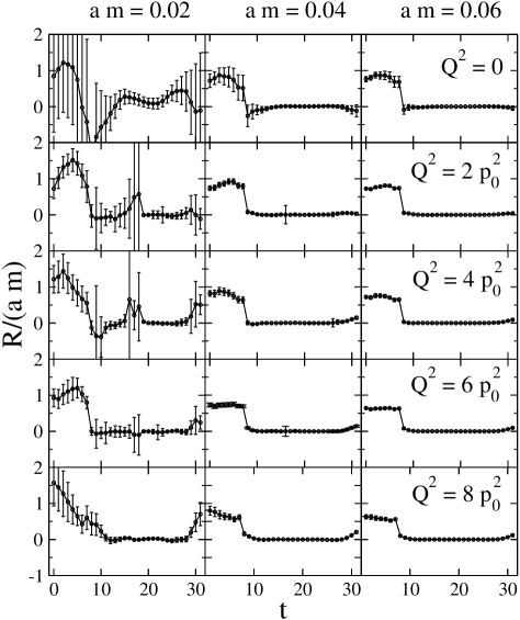
Figure 7: The ratio (13) for the matrix element (7) leading to the scalar form factor for all quark masses and transfer momenta considered (lattice size $16^{3}\times 32$).

Table 4: Values of the pion scalar form factor (lattice size $16^{3}\times 32$, $a=0.148$ fm, without disconnected contributions) obtained for different quark mass values.

$Q^{2}$[GeV]	$a\,m$=0.02	$a\,m$=0.04	$a\,m$=0.06
0	1.77(2.20)	1.30(39)	1.42(17)
0.546	2.09(53)	1.38(13)	1.31(6)
1.093	1.60(51)	1.31(13)	1.24(7)
1.639	1.61(56)	1.13(13)	1.04(7)
2.186	1.37(69)	1.03(16)	0.96(9)

The scalar form factor also has disconnected contributions which we disregard here (like it is often done due to the inherent technical complications of backtracking loops). We can notice from the upper plots in Fig. 7 and the upper line in Table 4 that the scalar form factor at zero momentum transfer divided by the quark mass has nearly the same value for all masses that we have simulated. This means that $\Gamma_{\pi}(0)\sim M_{\pi}^{2}\sim m$, as expected. We may determine the scalar radius squared from a fit to the $Q^{2}$-dependence of the scalar form factor (now explicitly normalized according to Eq. (8)).

In analogy to the vector form factor we expect that the scalar form factor in the space-like region is a decreasing but positive definite function. Thus a linear fit to its inverse seems appropriate. However, the result for the scalar radius squared is quite sensitive to this assumption. In Fig. 8 we compare the results of such a fit with those from a direct linear fit to our data in the space-like region and find a difference of almost 50%. In either case, the resulting value may then be extrapolated to the chiral limit.

ChPT relates the pion decay constant to the scalar form factor radius via

$$f_{\pi}/f=1+\frac{1}{6}\langle r^{2}\rangle_{s}M_{\pi}^{2}+\frac{13}{12}\xi+\mathcal{O}(\xi^{2})\;,$$ (18)

with

$$\xi=\left(\frac{M_{\pi}}{4\,\pi\,f_{\pi}}\right)^{2}\;.$$ (19)

The chiral expansion of the pion decay constant should behave like CoGaLe01

$$f_{\pi}/f=1+\xi\,\bar{\ell}_{4}+\mathcal{O}(\xi^{2})\;,$$ (20)

where the value $\bar{\ell}_{4}=-\ln(M_{\pi}^{2}/\Lambda^{2})$ depends on the intrinsic QCD scale $\Lambda$ and in CoGaLe01 it is suggested to use $\Lambda\approx 4\,\pi\,f_{\pi}$; in Ref. AnCaCo04 a value of $\bar{\ell}_{4}\approx 4.0\pm 0.6$ is quoted. Eq. (18) may be translated to

$$\langle r^{2}\rangle_{s}=\frac{3}{8\,\pi^{2}\,f_{\pi}^{2}}\,\left(\bar{\ell}_{4}-\frac{13}{12}+\mathcal{O}(\xi)\right)\;.$$ (21)

Recent values quoted in that context are $\langle r^{2}\rangle_{s}=0.61(4)\,\textrm{fm}^{2}$ AnCaCo04 or $0.75(7)\,\textrm{fm}^{2}$ Yn05 .

In QCD one expects correction terms with a logarithmic singularity in the valence quark mass $m$. As pointed out in Sh92 , the leading order logarithmic term $m\,\log m$ of ChPT involves quark loops that are however absent in the quenched case. There will be non-leading logarithmic terms, though. One therefore could allow a term $m^{2}\,\log m$ in the extrapolating fit. In the range of mass values studied here, the statistical accuracy of the data is too poor to render such an extrapolation significant. We therefore exhibit only the results of a constant extrapolation.

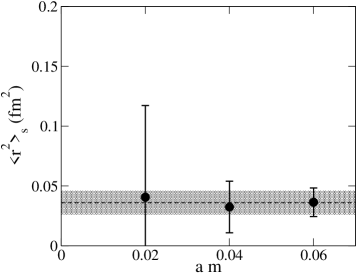
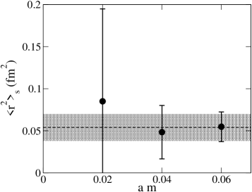
Figure 8: The mean square radius for the three available masses on the $16^{3}\times 32$ lattice for the scalar form factor. Upper plot: Determination from the linear fit to the values of $\Gamma_{\pi}(Q^{2})/\Gamma_{\pi}(0)$. Lower plot: Determination from the linear fit to the inverse of that ratio.

The resulting values (Fig. 8) are almost an order of magnitude smaller than for the electromagnetic case. From the data in Table 4, which takes into account the renormalization of the scalar operator, $Z_{S}=1.1309(9)$, as well as the kinematical factors, we obtain an average for the scalar radius of $\langle r^{2}\rangle_{s}=0.054(16)\;\textrm{fm}^{2}$ (based on the linear fit to the inverse form factor). This is also smaller than the values expected for full QCD. Results for the pion decay constant in a recent full QCD lattice calculation AuBeDe04 via (18) lead to the value $\langle r^{2}\rangle_{s}=0.5\pm 0.1~{}\textrm{fm}^{2}$. A corresponding analysis of the quenched BGR data GaHuLa05 gives again a small value, $0.08-0.13\;\textrm{fm}^{2}$. This seems to imply that $\langle r^{2}\rangle_{s}$ is very sensitive to quenching and possibly to the omission of the disconnected pieces.

A recent unquenched computation with $N_{f}=2$ clover fermions HaAoFu05 , which uses matrix elements of the scalar current and not the pion decay constant, quotes a larger value for the scalar radius squared, $\langle r^{2}\rangle_{s}=0.60(15)\;\textrm{fm}^{2}$. However, this number results from a ChPT-motivated extrapolation to data that is actually of smaller size and for pion masses $\geq$ 550 MeV.

VI Conclusions

Chirally improved fermions provide a framework for a first-principles lattice study of the hadron structure at comparatively small pion masses. In that context we present here our investigation of the vector and scalar form factors of the pion. We combine the method of HeKoLa04 (which for the vector form factor avoids calculation of the pion energy and thus removes one source of statistical error) with a GW type action, that allows one to reach small pion masses for comparatively small lattice size.

The vector form factor describes the electromagnetic structure and our results are generally consistent with expectations of its general form. In view of the quenched approximation we expect deviations from the experimental numbers. The vector charge radius indeed comes out 40% smaller than in experiment and the scalar radius is much lower than one would expect from unquenched calculations.

Further progress could be achieved - as usual - by using better statistics, more momenta, and larger lattices, both in lattice units (to study finite volume effects) and in physical units (to access lower transferred momenta).

- (1) G. Martinelli and C. T. Sachrajda, Nucl. Phys. B306, 865 (1988).
- (2) T. Draper, R. Woloshyn, W. Wilcox, and K.-F. Liu, Nucl. Phys. B318, 319 (1989).
- (3) Y. Nemoto (RBC collaboration) Nucl. Phys. Proc. Suppl. 129, 299 (2004).
- (4) J. van der Heide, J. Koch, and E. Laermann, Phys. Rev. D 69, 094511 (2004).
- (5) F. D. R. Bonnet, R. G. Edwards, G. T. Fleming, R. Lewis, and D. G. Richards, Phys. Rev. D 72, 054506 (2005).
- (6) A. M. Abdel-Rehim and R. Lewis, Phys. Rev. D 71, 014503 (2005).
- (7) D. Brömmel et al., Proc. Sci. LAT2005, 360 (2005).
- (8) P. H. Ginsparg and K. G. Wilson, Phys. Rev. D 25, 2649 (1982).
- (9) R. Narayanan and H. Neuberger, Phys. Lett. B 302, 62 (1993); Nucl. Phys. B443, 305 (1995).
- (10) H. Neuberger, Phys. Lett. B 417, 141 (1998); Phys. Lett. B 427, 353 (1998).
- (11) D. B. Kaplan, Phys. Lett. B 288, 342 (1992).
- (12) V. Furman and Y. Shamir, Nucl. Phys. B439, 54 (1995).
- (13) P. Hasenfratz and F. Niedermayer, Nucl. Phys. B414, 785 (1994).
- (14) C. Gattringer, Phys. Rev. D 63, 114501 (2001).
- (15) C. Gattringer, I. Hip, and C. B. Lang, Nucl. Phys. B597, 451 (2001).
- (16) C. Gattringer et al., Nucl. Phys. B677, 3 (2004).
- (17) C. Gattringer, M. Göckeler, P. Huber, and C. B. Lang, Nucl. Phys. B694, 170 (2004).
- (18) S. Capitani, C. Gattringer, and C. B. Lang, Proc. Sci. LAT2005, 126 (2005).
- (19) S. Hashimoto et al., Proc. Sci. LAT2005, 336 (2005).
- (20) G. J. Gounaris and J. J. Sakurai, Phys. Rev. Lett. 21, 244 (1968).
- (21) M. F. Heyn and C. B. Lang, Zeit. Phys. C7, 169 (1981).
- (22) J. F. de Trocóniz and F. J. Ynduráin, Phys. Rev. D 65, 093001 (2002).
- (23) H. Leutwyler, Electromagnetic form factor of the pion, hep-ph/0212324 (2002).
- (24) G. R. Farrar and D. R. Jackson, Phys. Rev. Lett. 43, 246 (1979).
- (25) S. Eidelman et al., Phys. Lett. B 592, 1 (2004).
- (26) B. Ananthanarayan, I. Caprini, G. Colangelo, J. Gasser, and H. Leutwyler, Phys. Lett. B 602, 218 (2004).
- (27) M. Lüscher and P. Weisz, Commun. Math. Phys. 97, 59 (1985); Err. 98, 433 (1985).
- (28) C. Gattringer, R. Hoffmann, and S. Schaefer, Phys. Rev. D 65, 094503 (2002).
- (29) C. Gattringer, P. Huber, and C. B. Lang, Phys. Rev. D 72, 094510 (2005); Proc. Sci. LAT2005, 121 (2005).
- (30) J. Volmer et al., Phys. Rev. Lett. 86, 1713 (2001).
- (31) C. J. Bebek et al., Phys. Rev. D 17, 1693 (1978).
- (32) S. R. Amendolia et al., Nucl. Phys. B277, 168 (1986).
- (33) P. Brauel et al., Z. Phys. C 3, 101 (1979).
- (34) G. Colangelo, J. Gasser, and H. Leutwyler, Nucl. Phys. B603, 125 (2001).
- (35) F. J. Ynduráin, Phys. Lett. B 612, 245 (2005).
- (36) S. R. Sharpe, Phys. Rev. D 46, 3146 (1992).
- (37) C. Aubin et al., Phys. Rev. D 70, 114501 (2004).