EFFECTIVE LATTICE ACTIONS FOR FINITE-TEMPERATURE YANG-MILLS THEORY

Abstract

We determine effective lattice actions for the Polyakov loop using inverse Monte Carlo techniques.

1 Introduction

As there are different notions of effective actions let us start right away with the definition we will employ throughout this presentation: Given an action $S=S[U]$ for some ‘microscopic’ degrees of freedom $U$ we define an action for ‘macroscopic’ degrees of freedom $X\equiv X[U]$ via the functional integral

$$e^{-S_{\mathrm{eff}}[{X}]}=\int\mathcal{D}\,U\,\delta({X}-{X}[U])\,e^{-S[U]}\;.$$ (1)

Hence we ‘integrate out’ ${U}$ in favor of ${X}$ which will guarantee that the actions ${S}$ and ${S_{\mathrm{eff}}}$ have the same matrix elements for the remaining degrees of freedom ${X}$. Typical examples of such effective actions are obtained if ${X}$ corresponds to low-energy degrees of freedom, like in chiral perturbation theory. Alternatively, ${X}$ may represent some order parameter (field) as is common in Ginzburg-Landau theory, for instance.

While this is all fairly straightforward in principle one encounters difficulties in practice: in general, the ${U}$-integration cannot be done analytically. Fortunately, there is a particularly elegant way out, encoded in the ‘effective field theory’ program. There, one argues that the effective action ${S_{\mathrm{eff}}[{X}]}$ should have the same symmetries as the ‘parent’ action ${S[U]}$ which suggests the ansatz

$$S_{\mathrm{eff}}[{X}]=\sum_{k}{\lambda_{k}}\,S_{k}[{X}]\;,$$ (2)

representing a systematic expansion in symmetric operators ${S_{k}}$ of increasing mass dimension (multiplied by inverse powers of the cutoff). The parameters ${\lambda_{k}}$ are then fixed via ‘phenomenology’.

Alternatively, one may try to ‘do the ${U}$-integration numerically’ on a lattice. However, on a lattice one can only calculate expectation values. So the question arises: How can one find effective actions from the latter? The answer is given in the next section.

2 Inverse Monte Carlo

Inverse Monte Carlo (IMC) avoids the functional integration in (1) by a detour consisting of three basic steps: first, generate configurations $U^{(i)}$, $i=1,\ldots,N$, via standard MC procedures. Second, calculate the configurations ${\big{\{}{X}^{(i)}\big{[}U^{(i)}\big{]}\big{\}}}$ and compute the expectation values $\langle O[{X}]\rangle_{S}=N^{-1}\sum_{i=1}^{N}O\big{[}{X}^{(i)}\big{]}$. Note that the $X$ variables are distributed according to $\exp(-S)$, i.e. the parent action. Third, in the IMC step proper, determine the effective couplings ${\lambda_{k}}$ via Schwinger-Dyson equations (SDEs) [1, 2]. The latter step requires some explanations.

Generically, the target space (where the $X$ variables ‘live’) will have some isometry leaving the metric invariant, ${{\hat{\mathcal{L}}_{X}}\,g^{ab}(X)=0}$, $\hat{\mathcal{L}}$ denoting the relevant Lie derivative. This entails an invariance of the functional measure, ${\mathcal{D}{X}\equiv\prod d{X}\,\sqrt{g({X})}}$, leading to path integral identities that can be cast into the SDEs

$$\sum_{k}\langle F{\hat{\mathcal{L}}_{X}}S_{k}\rangle_{S}{\lambda_{k}}=\langle{\hat{\mathcal{L}}_{X}}F\rangle_{S}\;,$$ (3)

where the ansatz (2) has been utilised. The former constitute an (overdetermined) linear system for the ${\lambda_{k}}$ which can be solved numerically. The arbitrary function ${F[{X}]}$, if properly chosen, can be used to fine-tune the associated numerics. An expensive (!) check of the solution can (and should) be done by testing the equality of the matrix elements calculated with both the parent and daughter actions, $\langle O\rangle_{S_{\mathrm{eff}}}\stackrel{{\scriptstyle?}}{{=}}\langle O\rangle_{S}$.

3 Polyakov-Loop Dynamics

In [3, 4] we have considered some particular examples of effective actions for the Polyakov loop based on suggestions in [5, 6, 7].

3.1 Generalities

At the risk of boring the experts we briefly review the physics of the Polyakov loop. This quantity is all-important for finite temperature Yang-Mills theory as it constitutes a gauge invariant order parameter for the confinement-deconfinement phase transition. The Polyakov loop is a traced holonomy (or Polyakov line),

$${{L}_{\mbox{\scriptsize\boldmath$x$}}[U]\equiv\frac{1}{N_{C}}\mbox{tr}_{F}\,{\mathfrak{P}}_{\mbox{\scriptsize\boldmath$x$}}[U]}\;,\quad{\mathfrak{P}}_{\mbox{\scriptsize\boldmath$x$}}[U]\equiv\prod_{t=1}^{N_{t}}U_{t,\mbox{\scriptsize\boldmath$x$};0}\;.$$ (4)

Introducing the Wilson coupling by $\beta=2N_{C}/g^{2}$ the theory assumes its confinement phase for $\beta<\beta_{c}$ with ${\langle{L}\rangle=0}$ and its deconfinement phase for ${\beta>\beta_{c}}$ with nonvanishing expectation value, ${\langle{L}\rangle\neq 0}$. The latter phase is characterised by a spontaneously broken centre symmetry generated by transformations under which $L$ transforms nontrivially, $L_{\mbox{\scriptsize\boldmath$x$}}\to z\,L_{\mbox{\scriptsize\boldmath$x$}}$, $z\in\mathbb{Z}(N_{C})$.

The critical behaviour is characterised by the Svetitsky-Yaffe conjecture [8, 9] which states that the effective theory describing finite-${T}$ ${SU(N_{C})}$ Yang-Mills theory in ${d+1}$ dimensions is a ${\mathbb{Z}(N_{C})}$ spin model in ${d}$ dimensions with short-range interactions. For ${SU(2)}$ this is well established on the lattice via comparison of critical exponents [10, 11].

For gauge group $SU(2)$, which we consider henceforth, $L$ is a real number between $-1$ and 1. This target space is somewhat nonstandard so that its isometry is not obvious. We therefore generalise to the group-valued variable, ${\mathfrak{P}}\equiv P^{\mu}\sigma_{\mu}\in SU(2)$. As $SU(2)\cong S^{3}$ its isometry is clearly an ${O(4)}$ symmetry generated by ‘angular momenta’ ${M^{\mu\nu}}$. Gauge invariance invariance then implies that the effective action can only depend on the zeroth component of $\mathfrak{P}$, ${S_{\mathrm{eff}}[{\mathfrak{P}}]\equiv S_{\mathrm{eff}}[{P^{0}}]\equiv S_{\mathrm{eff}}[{L}]}$. Restricting our identities to $P^{0}=L$ results in the following SDEs for the ansatz (2),

$$\sum_{k}\langle(1-{L}_{\mbox{\scriptsize\boldmath$x$}}^{2})GS_{k,\mbox{\scriptsize\boldmath$x$}}\rangle{\lambda_{k}}=\langle(1-{L}_{\mbox{\scriptsize\boldmath$x$}}^{2})G_{,\mbox{\scriptsize\boldmath$x$}}-3{L}_{\mbox{\scriptsize\boldmath$x$}}G\rangle\;,$$ (5)

where ${G_{,\mbox{\scriptsize\boldmath$x$}}\equiv\partial G/\partial{L}_{\mbox{\scriptsize\boldmath$x$}}}$ etc. Again, the functional $G$ is useful for fine-tuning. An optimal choice is to use the derivatives of the effective action, ${G\in\{S_{l,\mbox{\scriptsize\boldmath$y$}}\}}$, which are the operators appearing in the equation of motion for $L$. In this case the SDEs become relations between two-point functions of the Polyakov loop $L$. Again, they represent an exact, overdetermined linear system for the couplings ${\lambda_{k}}$. We still have not decided upon the concrete form of the effective action. This is somewhat of a problem, as the former is only mildly constrained by centre symmetry. The additional fact that $L$ is dimensionless allows for a plethora of operators $S_{k}$. Certainly, a further guiding principle is needed.

3.2 Effective Action from Character Expansion

Recall that any (gauge invariant) function on ${SU(N_{C})}$ can be expanded in terms of an adapted ‘Fourier’ basis, the group characters for representation $R$, $\chi_{R}[U]\equiv\mbox{tr}_{R}\,U$, with $U\in SU(N_{C})$. For ${SU(2)}$ we use the notation ${\chi_{p}}$ with ${p=2j}$ and ${j=\frac{1}{2},1,\frac{3}{2},\ldots,}$ denoting ‘color spin’. The lowest characters are the polynomials ${\chi_{1}}=2{L}$, $\chi_{2}=4{L}^{2}-1$, $\chi_{3}=8{L}^{3}-4{L}$, $\ldots$. If we impose ${\mathbb{Z}(2)}$ symmetry and reducibility of product representations we obtain the following systematic expansion for the effective action (see also [6, 12]),

$$S_{\mathrm{eff}}[{\chi}]=\sum_{\langle\mbox{\scriptsize\boldmath$x$}\mbox{\scriptsize\boldmath$y$}\rangle}\sum_{\scriptstyle pq\atop\scriptstyle{p-q\,\mathrm{even}}}\lambda_{pq}\,{\chi_{p}}[L_{\mbox{\scriptsize\boldmath$x$}}]\,{\chi_{q}}[L_{\mbox{\scriptsize\boldmath$y$}}]+\sum_{\mbox{\scriptsize\boldmath$x$}}\sum_{{p\,\mathrm{even}}}\lambda_{p0}\,{\chi_{p}}[L_{\mbox{\scriptsize\boldmath$x$}}]\;.$$ (6)

This action is a ${\mathbb{Z}(2)}$-symmetric sum over higher and higher ${SU(2)}$ representations including both nearest-neighbour (NN) hopping and potential terms. Before determining this action numerically it is worthwhile to study its consequences in mean-field approximation (MFA).

3.3 Mean-Field Approximation

If we restrict ourselves to the fundamental and adjoint representations (${p=1,2}$) and to hopping terms only we end up with the effective action (6) truncated such that it contains only couplings $\lambda_{11}$ and $\lambda_{22}$. This action will be denoted $T_{2}$ and implies a MF potential

$$V_{\mathrm{{MF}}}({\lambda},{\chi})\equiv-d\sum_{p=1,2}{\lambda_{pp}}{\chi_{p}}^{2}-\log z({\lambda},{\chi})$$

where $z$ is the single-site partition function. The two MF (or gap) equations are $\partial V_{\mathrm{{MF}}}/\partial{\chi_{p}}=0$, $p=1,2$, the solution of which yields the vacuum expectation values (VEVs) ${\bar{\chi}_{p}}$ of the characters. The latter are displayed in Fig. 1. The behaviour of $\bar{L}$ as a function of the coupling $\lambda_{11}$ implies the typical second-order phase transition (for $\lambda_{22}$ sufficiently large). Interestingly, the adjoint character $\bar{\chi}_{2}$ displays discontinuous behaviour as a function of $\lambda_{22}$ (for $\lambda_{11}$ sufficiently large). This behaviour, however, is located off the ‘physical region’ marked by the arrows. These point towards the couplings obtained by numerically matching to the Yang-Mills action via IMC. This is our next topic.

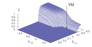
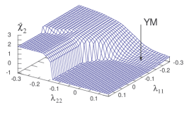
Figure 1: The MF predictions for the VEVs of the Polyakov loop $\bar{L}=\bar{\chi}_{1}/2$ (left) and the adjoint character $\bar{\chi}_{2}$ (right) as a function of the couplings $\lambda_{11}$ and $\lambda_{22}$.

3.4 Inverse Monte Carlo

We have simulated $SU(2)$ Yang-Mills theory on a $4\times 20^{3}$ lattice for Wilson coupling $\beta$ ranging between $1.2$ and $3.5$. The critical coupling is $\beta_{c}=2.30$. The associated ensembles have been matched to effective actions $S_{p}$ with representations $p\leq 3$, hence including up to five character terms and, accordingly, five effective couplings. Some results are presented in Fig. 2.

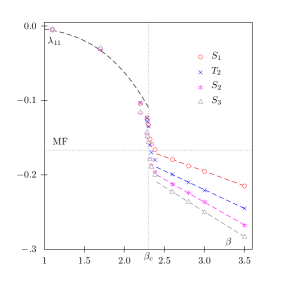
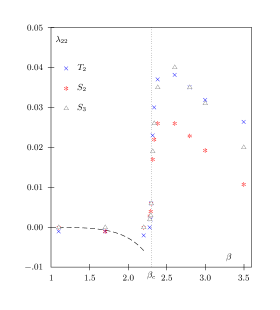
Figure 2: Effective couplings determined via IMC. Left: fundamental coupling ${\lambda_{11}}$, Right: adjoint coupling ${\lambda_{22}}$. Different symbols correspond to different truncated actions, $S_{1},\ldots,S_{3}$, see text. Dashed lines for small $\beta$ are strong-coupling results.

We see that both fundamental and adjoint couplings ($\lambda_{11}$ and $\lambda_{22}$) jump near the critical $\beta$. The effect of including potential terms and higher representations ($S_{2}$, $S_{3}$) is rather mild and visible mainly in the broken phase ($\beta>\beta_{c}$). The linear behaviour of $\lambda_{11}$ there is predicted by perturbation theory [13]. Finally, the MF critical coupling for an Ising type effective action $S_{1}$ ($\lambda_{11}$ only) is $\lambda_{11c}=-1/2d=-0.17$ is off by only a few percent.

To check the quality of our effective actions we have simulated them using the IMC values for the couplings and compared simple matrix elements namely the two-point functions (see Fig. 3).

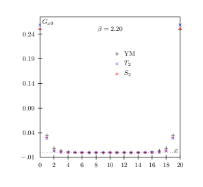
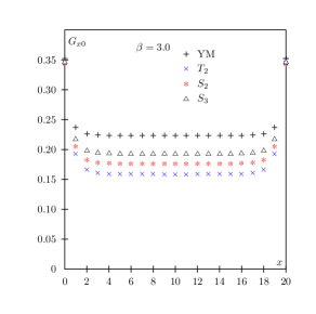
Figure 3: Two-point functions for $\beta=2.2$ (left) and $\beta=3.0$ (right).

We note that in the symmetric phase ($\beta=2.2$) the data for different truncations lie on top of each other and reproduce the Yang-Mills values. In the broken phase ($\beta=3.0$), however, the situation is different. Including higher representations leads to improvement but in particular the Yang-Mills plateau value (hence $\langle L\rangle$) is not reproduced.

To remedy this fault we have performed a brute-force calculation by also including next-to-nearest neighbour (NNN) interactions and a total of 14 different operators [3]. We find that generically the effective couplings decrease with the representation label $p$ (as above) and the distance of the sites connected by the operators. A comparison of the two-point functions now yields a near-perfect match (see Fig. 4).

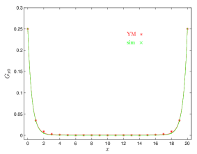
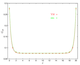
Figure 4: Two-point functions for $\beta=2.2$ (left) and $\beta=2.4$ (right) using 14 NN and NNN operators (“sim”).

4 Summary and Outlook

We have seen that inverse Monte Carlo based on Schwinger-Dyson equations can be a powerful method to numerically determine effective actions. Applying it to the Polyakov loop dynamics in ${SU(2)}$ yields ${\mathbb{Z}(2)}$-symmetric effective actions ${S_{\mathrm{eff}}[{L}]}$ describing the confinement-deconfinement phase transition in quite some detail. The matching to Yang-Mills is reasonable if NN character interactions are used and becomes near-perfect if one includes NNN interactions. Obvious extensions of this work will be to go to $SU(3)$ and to analyse explicit symmetry breaking terms (mimicking ‘fermions’). A study of the continuum limit will necessitate to renormalise the lattice Polyakov loop.

References

- [1] M. Falcioni et al., Nucl. Phys. B265, (1986) 187.
- [2] L. Dittmann, T. Heinzl and A. Wipf, JHEP 0212 (2002) 014 [arXiv:hep-lat/0210021].
- [3] L. Dittmann, T. Heinzl and A. Wipf, JHEP 0406 (2004) 005 [arXiv:hep-lat/0306032].
- [4] T. Heinzl, T. Kästner and A. Wipf, Phys. Rev. D 72 (2005) 065005 [arXiv:hep-lat/0502013].
- [5] B. Svetitsky, Phys. Rept. 132 (1986) 1.
- [6] M. Billo et al., Nucl. Phys. B 472 (1996) 163 [arXiv:hep-lat/9601020].
- [7] R. D. Pisarski, Phys. Rev. D 62 (2000) 111501 [arXiv:hep-ph/0006205].
- [8] B. Svetitsky and L.G. Yaffe, Nucl. Phys. B210, (1982) 423.
- [9] L.G. Yaffe and B. Svetitsky, Phys. Rev. D26 (1982) 963.
- [10] S. Fortunato et al., Phys. Lett. B 502 (2001) 321 [arXiv:hep-lat/0011084].
- [11] P. de Forcrand, M. D’Elia and M. Pepe, Phys. Rev. Lett. 86 (2001) 1438 [arXiv:hep-lat/0007034].
- [12] A. Dumitru et al., Phys. Rev. D 70 (2004) 034511 [arXiv:hep-th/0311223].
- [13] M. Ogilvie, Phys. Rev. Lett. 52 (1984) 1369.